Electronic Journal of Qualitative Theory of Differential Equations 2010, No. 7, 1-22;http://www.math.u-szeged.hu/ejqtde/
FUNCTION BOUNDS FOR SOLUTIONS OF VOLTERRA INTEGRO DYNAMIC EQUATIONS ON TIME SCALES
MURAT ADIVAR
Abstract. Introducing shift operators on time scales we construct the integro-dynamic equa-tion corresponding to the convoluequa-tion type Volterra differential and difference equaequa-tions in particular cases T= Rand T =Z. Extending the scope of time scale variant of Gronwall’s
inequality we determine function bounds for the solutions of the integro dynamic equation.
1. Introduction
In this paper, we are concerned with the investigation of function bounds for the solutions of integro dynamic equation of type
x∆(t) =−a(t)x(t) +
Z t
t0
b(δ−(s, t))x(s)∆s, t∈[t0,∞)∩T, (1.1)
which includes the following Volterra equations in particular cases:
• Volterra integro differential equation of convolution type: ForT=Rwithδ−(s, t) =t−s andt0 = 0
x′(t) =−a(t)x(t) +
Z t
0
b(t−s)x(s)ds, t∈[0,∞). (1.2)
• Volterra integral equation with nonconvolutional kernel: For T =R withδ−(s, t) =t/s andt0 = 1
x′(t) =−a(t)x(t) +
Z t
1
b(t
s)x(s)ds, t∈[1,∞). (1.3)
• Volterra integro difference equation of convolution type: For T = Z with δ−(s, t) = t−s+λand t0=λ
∆x(t) =−a(t)x(t) +
t−1 X
k=λ
b(t−k+λ)x(k), t∈[λ,∞)∩Z+, (1.4)
where ∆ is the forward difference operator.
• Volterra integro q−difference equation: ForT=qZ withδ−(s, t) =t/sand t0= 1
∆qx(t) =−a(t)x(t) + X
s∈[1,t)∩qZ
µ(s)b(t
s)x(s), t∈[1,∞)∩q
Z
, (1.5)
where ∆q is theq-difference operator given by ∆qx(t) =x(qt)(q−−1)tx(t).
2000 Mathematics Subject Classification. Primary 39A11, 39A12; Secondary 39A13, 45D05.
Key words and phrases. Function bounds, Gronwall’s inequality, Time Scales, Volterra integro dynamic equations.
Many papers have appeared in the literature on Volterra equations on particular time scales such as R,Z and qN. An early contribution to integro q-difference equations was made by Tr-jitzinsky [19]. In [15] and [16] Elaydi dealt with stability analysis of convolution type Volterra integro difference equations of the form (1.4). In [4], Becker derived an extension of Gronwall’s inequality to find function bounds for the solutions of Eq. (1.2), wherea, b: [0,∞) →Rare con-tinuous functions andbis nonnegative. Since the time scale theory provides a wide perspective for the unification of discrete and continuous analyses, Volterra integro dynamic equations on general time scales became topic of several research papers. For instance, boundedness of the solutions of nonlinear Volterra integro-dynamic equations on time scales has been investigated in [3] by means of nonnegative definite Lyapunov functionals on time scales. Furthermore, in [2], existence of periodic solutions of nonlinear system of Volterra type integro-dynamic equa-tions has been shown using the topological degree method and Schaefer’s fixed point theorem. However, to the best of our knowledge, function bounds for the solutions of Volterra integral equations of the form (1.3) has not been treated elsewhere before.
Motivated by the results of [4], we bring the integro dynamic equation (1.1) under investigation to obtain more general results which are not known even for the above mentioned particular cases. Some applications are also given to illustrate the usefulness of our results.
The remaining part of this paper is organized as follows: In the second section, we propose an extension of Gronwall’s inequality ( [7, Corollary 6.7, p.257]) on time scales. In the third section, we introduce the shift operatorsδ± to construct the kernel of integro dynamic equation (1.1). In the last section, we give several theorems and corollaries regarding the function bounds for the solutions of (1.1). Hence, it turns out that the results in Sections III and Section IV are valid only for the time scales containing an initial point t0 so that there exist shift operators
δ±(s, t) on [t0,∞)T.
For the sake of brevity, we assume familiarity with time scale calculus. For a comprehensive review on fundamental aspects of the theory we refer the reader to [7] and [8].
Throughtout the paper, we denote by σ and ρ the forward and backward jump operators, σ :T→T and ρ :T→T, defined by σ(t) := inf{s∈T:s > t} and ρ(t) = sup{s∈T:s < t}, respectively. A pointt∈Tis said to be right dense (right scattered) if σ(t) =t (σ(t) > t). We sayt∈Tis left dense (left scattered) if ρ(t) =t(ρ(t)< t). The graininness (step size) function µ :T→[0,∞) is defined by µ(t) := σ(t)−t. A function f :T → R is called rd-continuous if it is continuous at right dense points and its left sided limits exists (finite) at left dense points. We use the notation Crd to indicate the set of rd-continuous function on T. Hereafter, we shall
denote by [u, v)T the time scale interval [u, v)∩T. The intervals (u, v)T, [u, v]T, and (u, v]T are
defined similarly.
We list the following theorems which will be needed at several occasions throughout this study.
Theorem 1 (First Mean Value Theorem). [8, Theorem 5.41. p. 142] Let f and g be bounded and ∆ integrable functions on [u, v]T, and let g be nonnegative (or nonpositive) on [u, v]T. Let us set
m= inf{f(t) :t∈[u, v)T} and M = sup{f(t) :t∈[u, v)T}. Then there exists a real number Λ satisfying the inequalities m≤Λ≤M such that
Z t2
t1
f(t)g(t)∆t= Λ
Z t2
t1
g(t)∆t.
Theorem 2 (Intermediate Value Theorem). [7, Theorem 1.115] Assume x:T→Ris
continu-ous, u < v are points in T, and
x(u)x(v)<0.
Then there exists c∈[u, v)T such that either x(c) = 0 or x(c)xσ(c)<0.
Theorem 3 (Chain Rule). ([7, Theorem 1.93]) Assume f : T → R is strictly increasing and ˜
T:=f(T) is a time scale. Let g: ˜T→R. If f∆(t) and g∆˜(f(t)) exist for t∈Tκ, then (g◦f)∆= (g∆˜ ◦f)f∆.
Lemma 1. [8, Corollaries 1.15-16, p.5] Let f be a continuous function on [u, v]T that is ∆ differentiable on [u, v)T.
i. If f∆(t) = 0 for all t∈[u, v)
T, then f is a constant function on [u, v]T.
ii. f is increasing, decreasing, nondecreasing, and nonincreasing on [u, v]T if f∆(t) > 0,
f∆(t)<0, f∆(t)≥0, and f∆(t)≤0 for all t∈[u, v)
T, respectively.
Definition 1. [7, Definitions 2.25, 2.45] A function p:T→R is said to be regressive provided
that 1 +µ(t)p(t)6= 0 for all t∈Tκ. The set of all regressive rd-continuous functions p:T→ R
is denoted by R. We also denote byR+ the set R+ ={p ∈ R: 1 +µ(t)p(t) >0 for all t∈T}
of positively regressive functions.
Letp∈ R and µ(t)>0 for allt∈T. The exponential function onT is defined by
ep(t, s) = exp Z t
s
1
µ(z)Log(1 +µ(z)p(z)) ∆z
. (1.6)
The exponential function y(t) =ep(t, s) is the solution to the initial value problem y∆=p(t)y,
y(s) = 1. In particular, ifT=Z, then
ep(t, t0) = t−1 Y
s=t0
(1 +p(s)), t∈[t0,∞)T. (1.7)
Other properties of the exponential function are given by the following. Lemma 2. [6, Lemma 2.7.] If p, q∈ R, then
ep(t, t) = 1, ep(t, s) = 1/ep(s, t), ep(t, u)ep(u, s) =ep(t, s),
ep(σ(t), s)(1 +µ(t)p(t))ep(t, s), ep(s, σ(t)) =
ep(s, t)
1 +µ(t)p(t), e∆p(., s) =pep(., s), e∆p (s, .) = (⊖p)ep(s, .),
ep⊕q=epeq, ep⊖q=
ep
eq
.
Theorem 4. [7, Theorem 6.1] Let τ ∈T, y, f ∈Crd,and p∈R+. Then y∆(t)≤p(t)y(t) +f(t) for all t∈T
implies
y(t)≤y(τ)ep(t, τ) + Z t
τ
ep(t, σ(s))f(s)∆s for all t∈[τ,∞)T.
2. Gronwall’s inequality
There is no doubt that Gronwall’s inequality [14, p.293] plays a substantial role in the in-vestigation of stability and convergence properties of solutions of Volterra integral equations. The purpose of this section is to extend the scope of time scale analogue of Gronwall’s inequal-ity, which will be used to obtain function bounds for the solutions of Volterra integro-dynamic equations on time scales. A variant of Gronwall’s inequality on time scales is given as follows:
Theorem 5. [7, Corollary 6.7, p.257] Let y∈Crd and ω∈ R+, ω ≥0, and α∈R. Then
y(t)≤α+
Z t
t0
y(s)ω(s)∆s for all t∈[t0,∞)T (2.1)
implies
y(t)≤αeω(t, t0) for all t∈[t0,∞)T.
For more on Gronwall’s inequalities on time scales we refer to [7, p.256], [18], and [20]. One may easily see by setting T= [0,1]∪[2,∞),α= 3/2,t0= 0,ω(t) =−t, andy(t) = 1 for t∈[0,1] andy(t) = 0 for t∈[2,∞) that nonnegativity condition on the function ω in Theorem 5 cannot be omitted. However, in the next theorem, we keep positive regressivity condition ω ∈ R+ and rule out nonnegativity condition on ω by making more stringent assumption than (2.1). Therefore, we obtain important relaxations for the particular cases. For instance, if T = R, then µ(t) = 0, i.e., all functions ω : R→R are positively regressive, if T = Z, the functions ω : Z→R satisfying ω(t) > −1 for all t ∈ Z are positively regressive. That is, the following result is valid for all functions ω :R→R and for all functions ωe :Z→R satisfying
e
ω(t)>−1.
Theorem 6 (An extension of Gronwall’s inequality). Let f andγ be continuous functions on [t0, T)T where T ≤ ∞. Suppose that −γ ∈ R+.
i. If
f(t) +
t Z
τ
γ(s)f(s)∆s≤f(τ) (2.2)
for allτ, t∈[t0, T)T withτ ≤t, then
f(t)≤f(t0)e−γ(t, t0) for t∈[t0, T)T. (2.3)
ii. If
f(t) +
t Z
τ
γ(s)f(s)∆s≥f(τ)
for allτ, t∈[t0, T)T withτ ≤t, then
f(t)≥f(t0)e−γ(t, t0) for t∈[t0, T)T.
Hereafter, we present some results which are essential for the proof of Theorem 6.
Lemma 3. Let f, γ, and ξ be rd-continuous functions on [t0, T)T where T ≤ ∞. Let ξ∈ R+.
i. If γ(t)>0 for t∈(t0, T)T and
t Z
τ
γ(s)[f(s)−f(τ)eξ(s, τ)]∆s≤0 (2.4)
for allτ, t∈[t0, T)T with τ ≤t, then
f(t)≤f(t0)eξ(t, t0) for t∈[t0, T)T. (2.5)
ii. If γ(t)<0 for t∈(t0, T)T and
t Z
τ
γ(s)[f(s)−f(τ)eξ(s, τ)]∆s≥0 (2.6)
for allτ, t∈[t0, T)T with τ ≤t, then
f(t)≤f(t0)eξ(t, t0) for t∈[t0, T)T. (2.7) Proof. Let γ(t) > 0 for t ∈ (t0, T)T and (2.4) be satisfied. Suppose contrary that there is a
nonempty interval (t1, t2)T ⊂[t0, T)T, witht0 ≤t1< t2< T such that
f(t1)≤f(t0)eξ(t1, t0)
and
f(t)> f(t0)eξ(t, t0) for all t∈(t1, t2)T, (2.8)
i.e. (2.5) does not hold. Then using eξ(t, t1)eξ(t1, t0) =eξ(t, t0) we have
f(t)> f(t0)eξ(t, t1)eξ(t1, t0)≥f(t1)eξ(t, t1), (2.9)
which, along withγ >0, yields
t2
Z
t1
γ(t)[f(t)−f(t1)eξ(t, t1)]∆t >0, (2.10)
contradicting our assumption (2.4). The statement (ii.) can be verified by applying similar
arguments. The proof is complete.
One can similarly prove the next result by reversing the directions of the inequalities (2.8-2.10).
Corollary 1. Let f, γ, and ξ be rd-continuous functions on [t0, T)T where T ≤ ∞. Suppose that ξ ∈ R+.
i. If γ(t)>0 for t∈(t0, T)T and
t Z
τ
γ(s)[f(s)−f(τ)eξ(s, τ)]∆s≥0
for allτ, t∈[t0, T)T withτ ≤t, then
f(t)≥f(t0)eξ(t, t0) for t∈[t0, T)T.
ii. If γ(t)<0 for t∈(t0, T)T and
t Z
τ
γ(s)[f(s)−f(τ)eξ(s, τ)]∆s≤0
for allτ, t∈[t0, T)T with τ ≤t, then
f(t)≥f(t0)eξ(t, t0) for t∈[t0, T)T.
Now, we are ready to prove Theorem 6.
Proof of Theorem 6. We proceed by considering two cases: First, we consider the case in which γ is equivalently zero, strictly positive or strictly negative. Second, we handle the proof for the case whenγ changes sign.
Case I. If γ ≡ 0, then (2.3) follows from (2.2). Suppose γ(t) > 0 for all t ∈ (t0, T)T. For an
arbitrary τ ∈[t0, T)T define
xτ(t) = t Z
τ
γ(s)f(s)∆sfort∈[τ, T)T.
Invoking the differentiation rule ([7, Theorem 1.117]) we have x∆τ(t) =γ(t)f(t). Then multiplying both sides of (2.2) byγ(t), we obtain
x∆τ(t) +γ(t)xτ(t)≤f(τ)γ(t), (2.11)
Let us denote by pthe function
p(t) =⊖(−γ(t)).
Evidently, γ(t)>0 and −γ∈ R+ imply thatp= 1−γµγ >0 and that eσp(t, τ) = (1 +µp)ep(t, τ)>0
for all t∈(t0, T)T. Using the equality
eσp(t, τ)γ(t) = (1 +µ(t)p(t))γ(t)ep(t, τ)
=
1 + µ(t)γ(t) 1−µ(t)γ(t)
γ(t)ep(t, τ)
= γ(t)
1−µ(t)γ(t)ep(t, τ) =⊖(−γ(t))ep(t, τ)
=e∆p(t, τ),
and a multiplying both sides of (2.11) byeσp(t, τ) we find
eσp(t, τ)x∆τ (t) +eσp(t, τ)γ(t)xτ(t)≤f(τ)γ(t)eσp(t, τ),
which yields
eσp(t, τ)x∆τ (t) +e∆p (t, τ)xτ(t)≤f(τ)e∆p(t, τ),
and hence,
[ep(t, τ) (xτ(t)−f(τ))]∆≤0 for allt∈[τ, T)T.
Lemma 1 implies that the functionep(t, τ) (xτ(t)−f(τ)) is nonincreasing on [τ, T)T. That is,
ep(t, τ) (xτ(t)−f(τ))≤ep(τ, τ) (xτ(τ)−f(τ))
for all t∈[τ, T)T. Utilizingep(τ, τ) = 1 and xτ(τ) = 0, we obtain
ep(t, τ)xτ(t)≤f(τ)(ep(t, τ)−1).
Multiplying this inequality by e−γ(t, τ), we get
xτ(t)≤f(τ) (1−e−γ(t, τ)) =f(τ) t Z
τ
γ(s)e−γ(s, τ)∆s,
and therefore,
t Z
τ
γ(s)[f(s)−f(τ)e−γ(t, τ)]∆s≤0 for all t∈[τ, T)T. (2.12)
Since τ ∈[t0, T)T was arbitrary (2.12) holds for all t, τ ∈[t0, T)T satisfying τ ≤t. This is (2.4)
with ξ = −γ. Consequently, we obtain (2.3) by making use of Lemma 3. To get (2.3) in the case whenγ(t)<0 for allt∈(t0, T), it suffices to reverse direction of all the inequalities above
and use the fact that (2.6) implies (2.7).
Case II. Now, supposeγ changes sign. Hereafter, we will use continuity of the function γ on [t0, T)Tto show that the interval [t0, T)Tcan be partitioned into disjoint subintervals of the form
[tn−1, tn)T so thatγ is strictly negative, strictly positive, or identically zero on each of the open
intervals (tn−1, tn)T.
Let us define the setS ⊂[t0, T)T as follows
S ={t∈[t0, T)T:γ(t)γ(σ(t))<0}.
It is obvious that the setSconsists only of right scattered points of [t0, T)Tand can be expressed
as follows
S=∪t∈S[t, σ(t)).
Let us separate this set from [t0, T)T and define
K = [t0, T)T−S.
Denote the set of zeros ofγ inK byA, i.e.,
A={t∈K :γ(t) = 0}.
Since the single point set {0} is closed in R, we get by continuity ofγ that the set A=γ−1{{0}} ∩K ={t∈K :γ(t) = 0}
is closed in K (here, we are considering R with its standard topology and the subset K with the subspace topology inherited from the topology on R). Thus, the complement Ae =K−A of A inK is open in K. Consequently, the set Aeis composed of disjoint open intervals in K, each of which have one of the following forms: (a, b)∩Aeor [t0, b)∩A, wheree a, b∈[t0, T]T and
a < b. We conclude from Theorem 2 that on each of these open intervals, the function γ is either strictly positive or strictly negative. Because, if there exist two points t1, t2 ∈ (a, b)∩Ae
such that γ(t1)γ(t2) <0 then, Theorem 2 implies the existence of a point c∈ [t1, t2)∩Aesuch
that eitherγ(c) = 0 or γ(c)γ(σ(c))<0. This is not possible since Ae∩(A∪S) =∅. So, there is an increasing sequence (tn)n∈J of distinct points such that
∪n∈J[tn−1, tn)T = [t0, T)T
and the values of γ on (tn−1, tn) are always positive or always negative or always zero.
Quan-titative properties of the index set J depends on the function γ and the interval [t0, T)T , i.e.,
the set J can be either a finite set{1,2, ..., N} or the set of natural numbersN. From Case I we know that the inequality
f(t)≤f(tn−1)e−γ(t, tn−1) for t∈[tn−1, tn)T (2.13)
is satisfied, where [tn−1, tn)Tis any subinterval of the above mentioned partition of [t0, T)T. The
rest of the proof proceeds by induction. Suppose that (2.3) holds on [t0, tn−1)T=∪k=1n−1[tk−1, tk),
i.e.,
f(t)≤f(t0)e−γ(t, t0) for t∈[t0, tn−1)T. (2.14)
Iftn−1 is a left dense point, then continuity of both sides of (2.14) implies
f(tn−1)≤f(t0)e−γ(tn−1, t0). (2.15)
To see that (2.15) holds in the case whentn−1 is left scattered, assume thattn−2∈[t0, tn−1)T is
a point such that σ(tn−2) =tn−1 and define the function
F(t) :=f(t0)e−γ(t, t0). (2.16)
By (2.2) we have
f(tn−2)≥f(tn−1) + Z tn−1
tn−2
γ(s)f(s)∆s
=f(tn−1) +µ(tn−2)γ(tn−2)f(tn−2),
and therefore,
(1−µ(tn−2)γ(tn−2))f(tn−2)≥f(tn−1). (2.17)
It follows from (2.14), (2.16), and (2.17) that
F(tn−1) =F(tn−2) +µ(tn−2)F∆(tn−2)
=f(t0)e−γ(tn−2, t0){1−µ(tn−2)γ(tn−2)}
≥f(tn−2){1−µ(tn−2)γ(tn−2)} ≥f(tn−1).
Hence, (2.15) holds in any case. Thus, by (2.13) and (2.15) we get that f(t)≤f(tn−1)e−γ(t, tn−1)
≤f(t0)e−γ(tn−1, t0)e−γ(t, tn−1)
≤f(t0)e−γ(t, t0)
fort∈[tn−1, tn)T. This shows that (2.3) holds on the interval [t0, tn)T. By induction we conclude
that (2.3) holds on the entire interval [t0, T)T.
For the proof of second statement of theorem we reverse the directions of inequalities (2.2-2.3) and invoke Corollary 1 to modify the proof of the first statement accordingly. The proof is
complete.
3. Shift operators on time scales
In this section, we introduce the shift operators δ± : [t0,∞)T → Rto construct the
integro-dynamic equation
x∆(t) =−a(t)x(t) +
Z t
t0
b(δ−(s, t))x(s)∆s, t∈[t0,∞)T. (3.1)
An arbitrary time scale (e.g.,T=qN) does not have to includet−sand 0. Therefore, different than the kernelb(t−s) and the lower limit 0 of the integral in (1.2), we useb(δ−(s, t)) andt0 in
(3.1), respectively. An intuition for the determination of the shift operatorδ− can be developed by understanding the idea behind the use ofb(t−s) in (1.2). Informally, the expressionb(t−s) in (1.2) can be regarded as a shift (or delay) of the function b. However, since t−s /∈ qN
for the time scale T = qN
, the expression b(t−s) cannot be used as the shift of b. On the other hand, t/s ∈qN
for all t, s∈ qN
satisfying t≥ s≥ 1. Inspired by these examples and common properties of the operationst−sandt/s, we can construct backward shift operatorδ− on time scales. Similarly, we can describe properties of the forward shift operator δ+ considering the
properties of the operations t+sand ts.
Definition 2. Suppose we are given an initial point t0 ∈ T so that there exists operators δ± : [t0,∞)T×[t0,∞)T→[t0,∞)T satisfying the following properties:
P.1 δ+(s, t) ∈ [t0,∞)T for all s, t ∈ [t0,∞)T and δ−(s, t) ∈ [t0,∞)T for all s, t ∈ [t0,∞)T satisfyingt0 ≤s≤t,
P.2 Given a fixed elementT0 ∈[t0,∞)T, the functionsδ±are strictly increasing with respect to their second arguments, i.e.,
T0≤t < u implies δ±(T0, t)< δ±(T0, u),
P.3 If T1 < T2 for T1,T2 ∈ [t0,∞)T, then
δ−(T1, u)> δ−(T2, u) for all u∈[T2,∞)T and
δ+(T1, u)< δ+(T2, u) for all u∈[t0,∞)T,
P.4 δ−(t0, u) =δ+(t0, u) =u for all u∈[t0,∞)T,
P.5 δ+(t, s) =δ+(s, t) for all t, s∈[t0,∞)T,
P.6 δ−(δ+(s, u), δ+(u, v)) =δ−(s, v) for allu∈[t0,∞)T and s, v∈[t0,∞)T with s≤v,
P.7 δ+(δ−(s, u), δ−(u, v)) =δ−(s, v) for alls, u, v ∈[t0,∞)T satisfyings≤u≤v.
Then the operatorsδ−and δ+ associated with the initial pointt0 are called backward and
forward shift operators on[t0,∞)T, respectively.
Generalized shifts and the associated geometry on a general time scale were first dealt with in [11]. Also, generalized convolution on time scales was treated by [13]. Afterwards, in [10, Definition 2.1] shift operators was defined to propose convolution on time scales. Note that the shift operatorsδ± defined here are different than the ones in the above mentioned literature.
Example 1. The operators δ± described in (1.2-1.5) satisfy P.1-7 on the given time scales.
This example shows that we can define different type shift operators on the same time scale. For instance, onT=R, we have the shift operatorsδ±(s, t) =t±sandbδ±(s, t) =ts±1 with the initial points 0 and 1, respectively.
Making use of properties P.1-7, we obtain the following result.
Lemma 4. i. For a fixed T ∈(t0,∞)T we have
δ+(T, t)> δ+(t0, t) =t for allt∈[t0,∞)T and
δ−(T, t)< δ+(t0, t) =t for allt∈[T,∞)T.
ii. u=δ−(s, t) implies t=δ+(u, s) for allt∈[t0,∞)T and s, u∈[t0, t]T,
iii. u=δ−(s, t) implies s=δ−(u, t) for allt∈[t0,∞)T and s, u∈[t0, t]T,
iv. δ−(δ−(s, t), t) =sfor all s, t∈[t0,∞)T satisfyings≤t,
v. δ+(δ−(s, t), s) =t for all s, t∈[t0,∞)T satisfyings≤t,
vi. δ−(s, δ+(s, u)) =u for all s, u∈[t0,∞)T,
vii. δ−(u, u) =t0 for allu∈[t0,∞)T.
Proof. (i) follows from P.2 and P.3. To show (ii), use P.4-5 and P.7 to obtain δ+(u, s) =δ+(δ−(s, t), δ−(t0, s))
=δ+(δ−(t0, s), δ−(s, t)) =δ−(t0, t) =t.
For the proof of (iii) we use (ii) to get
u=δ−(s, t)⇒t=δ+(u, s).
This, along with P. 4 and P.6, yields
s=δ−(t0, s) =δ−(δ+(t0, u), δ+(u, s)) =δ−(u, t). (iv) is direct implication of (iii) sinceu=δ−(s, t) implies s=δ−(u, t) and
s=δ−(u, t) =δ−(δ−(s, t), t).
(v) is obtained by assumingu=δ−(s, t), using (ii), i.e., t=δ+(u, s), and
t=δ+(u, s) =δ+(δ−(s, t), s). To verify (vi) takeu=δ−(s, t) use (ii) to gett=δ+(s, u) and
u=δ−(s, t) =δ−(s, δ+(s, u)).
(vii) is proven by substitutings=v=t0 in P.6. The proof is complete.
Notice that shift operatorsδ±are defined once the initial pointt0 ∈Tis known. For instance,
we choose the initial pointt0 = 0 to define shift operatorsδ±(s, t) =t±sonT=R. However, if we take the initial pointλ∈(0,∞) then we can define new shift operators byδe±(s, t) =t∓λ±s and in terms ofδ± as
e
δ±(s, t) =δ∓(λ, δ±(s, t)).
Example 2. In the following table, we give several particular time scales to show the change in the formula of shift operators as the initial points change.
T=N1/2 T=hZ T= 2N
t0 0 λ 0 hλ 1 2λ
δ−(s, t) √
t2−s2 √t2+λ2−s2 t−s t+hλ−s t/s 2λts−1
δ+(s, t)
√
t2+s2 √t2−λ2+s2 t+s t−hλ+s ts 2−λts
where λ∈Z+, N1/2={√n:n∈N}, 2N={2n:n∈N}, and hZ={hn:n∈Z}.
In general, let T be a time scale with shift operators δ± associated with initial point t0. Choosing a new initial point λ∈[t0,∞)T, we can define the new shift operators eδ± associated
withλby
e
δ−(s, t) =δ+(λ, δ−(s, t)), (3.2)
e
δ+(s, t) =δ−(λ, δ+(s, t)). (3.3)
Using P.1-7, one may easily verify that the new shift operatorsδe±satisfy the following properties:
e
P.1 eδ+(s, t) ∈ [λ,∞)T for all s, t ∈ [λ,∞)T and eδ−(s, t) ∈ [λ,∞)T for all s, t ∈ [λ,∞)T
satisfyingλ≤s≤t,
e
P.2 Given a fixed elementT0∈[λ,∞)T, the functionsδe±are strictly increasing with respect
to their second arguments, i.e.,
T0 ≤t < u implieseδ±(T0, t)<δe±(T0, u), e
P.3 If T1 < T2 forT1,T2 ∈[λ,∞)T, then
e
δ−(T1, u) >eδ−(T2, u) for all u∈[T2,∞)T
and
e
δ+(T1, u)<eδ+(T2, u) for allu∈[λ,∞)T,
e
P.4 eδ−(λ, u) =eδ+(λ, u) =u for allu∈[λ,∞)T,
e
P.5 eδ+(t, s) =eδ+(s, t) for all t, s∈[λ,∞)T,
e
P.6 eδ−(eδ+(s, u),eδ+(u, v)) =eδ−(s, v) for allu∈[t0,∞)T and s, v∈[t0,∞)T with s≤v,
e
P.7 eδ+(eδ−(s, u),eδ−(u, v)) =eδ−(s, v) for alls, u, v ∈[t0,∞)T satisfying s≤u≤v.
Moreover, the properties given in Lemma 4 are also valid for the operators eδ±.
4. Function Bounds for Solutions of Volterra Equations
Hereafter, we suppose that T is a time scale including an initial pointt0 so that there exists shift operators δ± satisfying properties P.1-7 in Definition 2. Let a, b : [t0,∞)T → R be two
continuous functions with b(t) ≥ 0 for all t ∈ [t0,∞)T and −a ∈ R+.Hereafter, we denote by
x(t) :=x(t, t0, x0) the unique differentiable solution of
x∆(t) =−a(t)x(t) +
t Z
t0
b(δ−(s, t))x(s)∆s (4.1)
satisfying x(t0) =x0. For the existence and boundedness of such a solution we refer the reader
to [1], [3], and [12]. For brevity, we shall use the notationx(t) instead ofx(t, t0, x0).
Theorem 7. Let γ be defined by
γ(u) =a(u)−
u Z
t0
b(δ−(s, u))ep(u, s)∆s, (4.2)
where p is given by
p(t) =⊖(−a(t)). (4.3)
i. If x0 ≥0, then
x0e−a(t, t0)≤x(t)≤x0e−γ(t, t0) for all t∈[t0,∞)T. (4.4)
ii. If x0 <0, then
x0e−γ(t, t0)≤x(t)≤x0e−a(t, t0) for all t∈[t0,∞)T. (4.5) Proof. First we show that x(t) is nonnegative for all t ∈ [t0,∞)T. If x0 = 0, then x(t) ≡ 0 is
the unique differentiable solution of (4.1) and (4.4) holds for such x. Hereafter, we assume that x0 >0. Let the set Ω be defined by
Ω :={t∈T:t > t0 and b(s) = 0 for alls∈[t0, t)T}.
If Ω is unbounded above, then b(t) = 0 for all t∈[t0,∞)T. Hence, (4.1) turns into
x∆(t) =−a(t)x(t) and x(t0) =x0 (4.6)
for all t∈[t0,∞)T, which has the unique solution
x(t) =x0e−a(t, t0). (4.7)
The solution (4.7) can also be derived from the fact that (4.6) implies
x(t) +
t Z
τ
a(u)x(u)∆u=x(τ)
for all τ, t satisfying t0 ≤τ ≤t. This, along with Theorem 6, yields (4.7). On the other hand,
by (P.1-P.4) we get that
u=δ−(t0, u)≥δ−(s, u)≥δ−(u, u) =t0 fort0≤s≤u, (4.8)
i.e., δ−(s, u) ∈[t0, u)T for t0 ≤s≤u. That is, if Ω is unbounded abaove, then b(δ−(s, u)) = 0
for all s∈[t0, u)T and
γ(u) =a(u) for all u∈[t0,∞)T, (4.9)
by (4.2). Thus, (4.4) follows from (4.7) and (4.9).
It remains to show that (4.4) is satisfied whenever Ω is empty or bounded above. To do so, we first need to show that x(t)>0 for allt∈[t0,∞)T. Define the non-negative numberT ≥t0 by
T =
t0 if Ω =∅
sup Ω otherwise .
IfT =t0, thenx(T) =x0>0. LetT > t0 andb(T)>0. IfT is left scattered, then there exists
a right scattered pointbt∈[t0, T)T such thatσ(t) =b T. Since b(t) = 0 for all t∈[t0,bt]T we have
x(bt)>0. Using (4.1) and the formula
xσ(t) =x(t) +µ(t)x∆(t), (4.10)
(see [7, Theorem 1.16 (iv)]), we find
x(T) =x(bt) +µ(bt)x∆(bt) = 1−a(bt)µ(bt)x(bt)>0.
If T ∈(t0,∞)T is a left dense point, then the inequalityx(t) =x0e−a(t, t0)>0 on [t0, T)T and
continuity of x implyx(t)>0 for all [t0, T]T.
To see nonnegativity of x(t) on the interval (T,∞)T it suffices to prove that the set M− given
by
M−:={t∈(T,∞)T:x(t)<0}
is empty. Suppose contrary that M−6=∅and denote byt1 the real number
t1:= infM−.
Henceforth, we show thatt1 ∈M−, i.e., x(t1)<0. It follows from continuity ofxthat
x(t1)≤0,
in which the case x(t1) = 0 leads to a contradiction in the sign of x∆(t1). To see this, let
x(t1) = 0. Thus,t1 is right dense, and hence,M− includes a continuous interval (t1, a) on which
x is nonincreasing, i.e., x∆(t
1)≤0. On the other hand, from (4.1) and Theorem 1 we arrive at
x∆(t1) =−a(t1)x(t1) + Z t1
t0
b(δ−(s, t1))x(s)∆s
≥
Z T
t0
b(δ−(s, t1))x(s)∆s
= Λ1 Z T
t0
b(δ−(s, t1))∆s
where Λ1 is a real number satisfying
m1 ≤Λ1 ≤M1 (4.11)
in which m1 and M1 are given by
m1 = min{x(t) :t∈[t0, T]T} and M1= max{x(t) :t∈[t0, T]T}
Evidently,
m1>0. (4.12)
On the other hand, similar to (4.8) we get thatt0 ≤s≤T implies
t1 =δ−(t0, t1)≥δ−(s, t1)≥δ−(T, t1)> δ−(t1, t1) =t0.
This shows thatb(δ−(s, t1)) is not equally zero on the interval [t0, T)T. From (4.11-4.12) we find
Λ1 Z T
t0
b(δ−(s, t1))∆s >0.
Therefore, we have t1 ∈ M−, i.e., x(t1) < 0. Since x(T)x(t1) < 0, Theorem 2 guarantees the
existence of a c∈[T, t1) such that
x(c) = 0 or x(c)x(σ(c))<0,
wherex(c)x(σ(c))<0 is not possible. To see this, we show that the set given by D:={t∈[T, t1)T:x(t)xσ(t)<0}
is empty. If there exists at∗ ∈D, thenx(t∗)>0 andx(σ(t∗))<0.Since t
1= infM−∈M− we have
σ(t∗) =t1 ∈/D.
This along with−a∈ R+, i.e., 1−µ(t)a(t)>0, implies
x(t1) =x(σ(t∗)) ={1−µ(t∗)a(t∗)}x(t∗) +µ(t∗) Z t∗
t0
b(δ−(s, t∗))x(s)∆s≥0,
where we also used (4.1) and (4.10). This leads to a contradiction. Hence, we havex(c) = 0 for a c∈(T, t1)T. This shows that the set
M0 ={t∈(T, t1)T :x(t) = 0}
is non-empty. Let
η= supM0.
It follows from continuity ofxthatη∈M0. SinceD=∅, as a consequence of Theorem 2, there
cannot be any element t∈(η, t1)T such thatx(t)>0. Thus, (η, t1)T =∅and thenx is strictly
decreasing on [η, t1)T, i.e., x∆(η)<0 by Lemma 1. However, we get from Theorem 1 that
x∆(η) =−a(c)x(η) +
η Z
t0
b(δ−(s, η))x(s)∆s
= Λ
η Z
t0
b(δ−(s, η))∆s≥0,
where Λ is a real number satisfying 0≤Λ≤sup{x(t) :t∈(t0, η)T}. We obtain this
contradic-tion by assuming thatM 6=∅. Consequently,M−=∅, i.e.,x(t)≥0 for all t∈[t0, T)T. Taking
the integral in (4.1) from τ to t, we arrive at
x(t)−x(τ) =−
t Z
τ
a(u)x(u)∆u+
t Z
τ u Z
t0
b(δ−(s, u))x(s)∆s∆u. (4.13)
Having bothb(δ−(s, u)) andx(s) are nonnegative we obtain
x(t) +
t Z
τ
a(u)x(u)∆u≥x(τ), (4.14)
for all t, τ ∈[t0,∞)T satisfying τ ≤t. By Theorem 6, we find the lower bound
x(t)≥x0e−a(t, t0) for t∈[t0,∞)T. (4.15)
Using this lower bound we can write
x(s)≤ep(u, s)x(u) for all u≥s≥t0, (4.16)
wherep is as in (4.3). Combining (4.13) and (4.16), for allτ, t∈[t0,∞)T withτ ≤t
x(t)≤x(τ)−
t Z
τ
a(u)x(u)∆u+
t Z
τ u Z
t0
b(δ−(s, u))ep(u, s)x(u)∆s∆u
=x(τ)−
t Z
τ a(u)−
u Z
t0
b(δ−(s, u))ep(u, s)∆s
x(u)∆u
=x(τ)−
t Z
τ
γ(u)x(u)∆u, (4.17)
where γ is defined as in (4.2). Note that −γ ∈ R+ since −a ∈ R+ and b(δ
−(s, u)) ≥0 for all s∈[t0, u)T. Theorem 6 yields
x(t)≤x0e−γ(t, t0). (4.18)
Consequently, the result (4.4) follows from inequalities (4.15) and (4.18).
To see that (4.5) holds for x0 =x(t0) <0, it is enough to employ (4.4) by taking into account
that−x(t) is the unique solution of Eq. (4.1) satisfying the initial condition −x(t0) =−x0>0.
The proof is complete.
Letλ∈[t0,∞) be any fixed element. Consider the integro-dynamic equation
x∆(t) =−a(t)x(t) +
t Z
λ
b(δ−(s, t))x(s)∆s. (4.19)
Henceforth, we denote by X(t) the unique differentiable solution X(t, λ, X0) of Eq. (4.19)
satisfying the initial conditionX(λ) =X0.
In the next corollary, we shall provide lower and upper bounds forX(t) by using the results of Theorem 7. To be able to employ Theorem 7 in the analysis, first of all the kernel of the integral term in (4.19) should include the shift operator associated with λ. As we have mentioned in Section 3 we may move the initial pointt0 toλ, and define the new shift operatorsδe±associated withλas in (3.2) and (3.3), respectively. Let us define the functioneb: [λ,∞)T→[0,∞) by
eb(u) =b(δ−(λ, u)). (4.20)
It is obvious thateb(u)≥0 for all [λ,∞)T. Also we get by Lemma 4 (vi) and (3.2) that
eb(eδ−(s, t)) =b(δ−(λ,eδ−(s, t))) =b(δ−(λ, δ+(λ, δ−(s, t)))) =b(δ−(s, t)).
Hence, we can rewrite Eq. (4.19) as follows
x∆(t) =−a(t)x(t) +
t Z
λ
eb(δe−(s, t))x(s)∆s. (4.21)
Define the functions
e
γ(u) =a(u)−
u Z
λ
eb(eδ−(s, u))ep(u, s)∆s, (4.22)
and
q(u) =a(u)−
u Z
λ
eb(eδ−(s, u))∆s,
respectively. Note thateb=b, and hence, eγ =γ whenever λ=t0.
Corollary 2. Let a, b : [t0,∞)T → R be two continuous functions with b(t) ≥ 0 for all t ∈
[t0,∞)T and let −a∈ R+. Let the functioneb be given by (4.20). Suppose
a(u)≥
u Z
λ
eb(δe−(s, u))ep(u, s)∆s (4.23)
for allu ∈[λ,∞)T.
i. If X0 ≥0, then X(t) is nonincreasing on [λ,∞)T and
X0e−q(t, λ) ≤X(t)≤X0e−γe(t, λ) (4.24) for allt∈[λ,∞)T,
ii. If X0 <0, then X(t) is nondecreasing on [λ,∞)T and
X0e−eγ(t, λ)≤X(t)≤X0e−q(t, λ) (4.25)
for allt∈[λ,∞)T.
Proof. Considering Eq. (4.21), we will proceed in a way similar to proof of Theorem 7. First we will show that (4.24) holds. By (4.23), we know thateγ(t)≥0 for allt∈[λ,∞)T. As in Theorem
7, we can show that ifX0≥0, thenX(t)≥0 for all t∈[λ,∞)T. Similar to (4.17) we have
X(t)≤X(τ)−
t Z τ a(u)X(u)∆u+ t Z τ u Z λ
eb(eδ−(s, u))ep(u, s)X(u)∆s∆u
=X(τ)−
t Z
τ a(u)−
u Z
λ
eb(δe−(s, u))ep(u, s)∆s
X(u)∆u
=X(τ)−
t Z
τ e
γ(u)X(u)∆u,
for all t, τ ∈[λ,∞)T with τ ≤t. Hence,
X(u)≤X(s) for all u, s∈[τ,∞)T withs≤u.
This shows monotonicity of solutions. Substituting X(u) for X(s) in
X(t)−X(τ) =−
t Z τ a(u)X(u)∆u+ t Z τ u Z λ
eb(eδ−(s, u))X(s)∆s∆u
we arrive at
X(τ)≤X(t) +
t Z
τ a(u)−
u Z
λ
eb(eδ−(s, u))∆s
X(u)∆u=X(t) +
t Z
τ
q(u)X(u)∆u (4.26)
for all t, τ ∈[λ,∞)T with τ ≤t. Since −a∈ R+ and
u Z
λ
eb(eδ−(s, u))≥0 for allu∈[λ,∞)T,
we have −q∈ R+ on [λ,∞)
T. Applying Theorem 6 to (4.26), we get the lower bound
X0e−q(t, λ)≤X(t).
The upper bound in (4.24) can easily be obtained by using the similar arguments to the ones in (4.16-4.18). In the case X0 <0, (4.25) can be proved as it is done at the end of Theorem 7.
The proof is complete.
We need the condition (4.23) to guarantee the monotonicity of the solutions of (4.19). In the following corollary, we rule out this condition to obtain weaker conditions leading to lower and upper bounds for the solutions of (4.19).
Corollary 3. Let a, b : [t0,∞)T → R be two continuous functions with b(t) ≥ 0 for all t ∈
[t0,∞)T and let −a∈ R+.
i. If X0 ≥0, then
X0e−a(t, λ)≤X(t)≤X0e−eγ(t, λ) (4.27)
for allt∈[λ,∞)T,
ii. If X0 <0, then
X0e−eγ(t, λ)≤X(t)≤X0e−a(t, λ) (4.28)
for allt∈[λ,∞)T.
Proof. Notice that this corollary is equivalent to Theorem 7 whenλ =t0. To verify (4.27) for
λ > t0, we proceed in a way similar to proof of Corollary 2. The upper bound in (4.27) can be
obtained as it is done in the proof of Corollary 2. So, we only need to find the lower bound. From (4.21) we have
X(t)−X(τ) =−
t Z
τ
a(u)X(u)∆u+
t Z
τ u Z
λ
eb(eδ−(s, u))X(s)∆s∆u,
in whichX(t)≥0 wheneverX0≥0 by Theorem 7. Since the functionebis also nonnegative, we
find
X(t) +
t Z
τ
a(u)X(u)∆u≥X(τ), for all t, τ ∈[λ,∞)T withτ ≤t,
and therefore, by Theorem 6
X0e−a(t, λ)≤X(t).
The proof is completed as we did in the proof of Theorem 7.
Considering [4, Examples 3.2, 3.7] one may see the consistency of the results with the special case T=R (see also [5]). For the case T=Z the following example numerically illustrates the bounds obtained in Corollary 3.
Example 3. Let us take T=Z, a(t) = 1/2, δ−(k, t) =t−k, and
b(t−k) = 1
2t−k(t−k+ 6)(t−k+ 5)
to construct the convolution type Volterra integro difference equation
x(t+ 1) = x(t)
2 +
t−1 X
k=1
x(k)
2t−k(t−k+ 6)(t−k+ 5), t∈[1,∞)Z. (4.29)
It is obvious from (1.7) that
e−a(t,1) = (0.5)t−1
and
e
γ(t) = 1 2 −
t−1 X
k=1
1
(t−k+ 6)(t−k+ 5)
= 1 3 +
1 t+ 5.
Hence,
e−eγ(t,1) = t−1 Y
k=1
2 3−
1 k+ 5
.
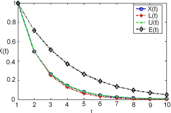
LetX(t) denote the solution of (4.29) satisfyingX(1) = 1. Using MATLAB 6.12, the numerical values of the functions L(t) := e−a(t,1) = (0.5)t−1, X(t), U(t) := e−eγ(t,1), and E(t) :=
exp(−13(t−1)) for t∈[1,10]Z are computed as follows:
t L(t) X(t) U(t) E(t)
1 1 1 1 1
2 0,5 0,5 0,5 0,7165
3 0,25 0,2619 0,2619 0,5134 4 0,125 0,1414 0,1419 0,3679 5 0,0625 0,0778 0,0788 0,2636 6 0,0313 0,0433 0,0447 0,1889 7 0,0156 0,0243 0,0257 0,1353 8 0,0078 0,0137 0,015 0,097 9 0,0039 0,0077 0,0088 0,0695 10 0,002 0,0044 0,0053 0,0498
As depicted in Figure 1, graphs of the functionsL and U lie alongside that of X(t).
Fig. 1. Upper and lower bounds for a solutionX(t) of (4.29)
We continue this section by listing some remarks. The following remark can be found in [9]. Remark 1. (1) For a nonnegative ϕwith −ϕ∈ R+, we have the inequalities
1−
Z t
s
ϕ(u)≤e−ϕ(t, s)≤exp
−
Z t
s
ϕ(u)
for all t≥s
(2) If ϕis rd-continuous and nonnegative, then
1 +
Z t
s
ϕ(u)≤eϕ(t, s)≤exp Z t
s
ϕ(u)
for all t≥s
It follows from (1.6) thateϕ(t, s)>0 for ϕ∈ R+ and t≥s. One may derive the next result
using Remark 1.
Remark 2. (1) If ϕ∈ R+ andϕ(t)<0for all t∈T, then for all s∈Twith s≤t we have
0< eϕ(t, s)≤exp Z t
s
ϕ(r)∆r
<1.
(2) If ϕ∈ R+, then
0< eϕ(t, s)≤exp Z t
s
ϕ(r)∆r
(4.30)
for allt∈[s,∞)T.
For more on inequalities regarding the exponential function on time scales see also [7, Theorem 2.44, p.66].
Corollary 4. In addition to all assumptions of Corollary 3 suppose also that
lim
t→∞
Z t
λ e
γ(s)∆s=∞, (4.31)
then for any X0 ∈R, X(t) =X(t, λ, X0) tends to zero as t→ ∞.
Proof. Sinceeb takes only nonnegative values, we get by (4.22) that
a(u)≥eγ(u) for allu∈[λ,∞)T, (4.32)
and hence,
1−µ(u)a(u) ≤1−µ(u)eγ(u) for all u∈[λ,∞)T,
i.e., −eγ ∈ R+. On the other hand, by (4.27), (4.28), and (4.30) we obtain
0≤X(t)≤X0exp − Z t λ e γ(s)∆s
forX0≥0
and
X0exp − Z t λ e γ(s)∆s
≤X(t)<exp
− Z t λ e γ(s)∆s
for X0 <0
for all t∈[λ,∞)T. The proof follows from (4.31).
Remark 3. In the particular case T=Z, Corollary 4 provides alternative conditions implying asymptotic stability of zero solution of convolution type Volterra difference equations
xn+1=axn+ n−1 X
s=0
bn−sxs, n≥0,
handled in[15, Theorem 1.1] ( see also[16] and [17]).
Corollary 5. In addition to assumptions of Corollary 2 suppose also that there exists an ε >0 such that
a(u)−
u Z
λ
eb(eδ−(s, u))ep(u, s)∆s≥ε (4.33)
holds for allu∈[λ,∞)T.
i. IfX0 >0, then the solutionX(t) =X(t, λ, X0)of (4.19) is strictly decreasing on[λ,∞)T and
X0e−q(t, λ)≤X(t)≤X0exp (−ε(t−λ)) (4.34)
for allt∈[λ,∞)T,
ii. IfX0 <0, then the solution X(t) =X(t, λ, X0)of (4.19) is strictly increasing on[λ,∞)T and
X0exp (−ε(t−λ))≤X(t)≤X0e−q(t, λ) (4.35)
for allt∈[λ,∞)T.
Proof. Upper and lower bounds in (4.34) follow from (4.24), (4.30), and (4.33). The upper bound in (4.35) is obtained from (4.25). On the other hand, for X0 <0, (4.30) yields
e−eγ(t, λ)≤exp − Z t λ e γ(s)∆s
≤exp (−ε(t−λ)),
and
X0e−eγ(t, λ)≥X0exp − Z t λ e γ(s)∆s
≥X0exp (−ε(t−λ)).
Hence, the lower bound in (4.35) can be found by using (4.25). Note that (4.33) implies thateγis strictly positive. Thus, by (4.17) the solution X(t) =X(t, λ, X0) of (4.19) is strictly decreasing
on [λ,∞)T provided X0 > 0. For X0 <0, monotonicity of X(t) = X(t, λ, X0) is obtained by
applying the same type of argument that ends the proof of Theorem 7. The proof is complete. It is obvious that the functioneγ in Example 3 satisfies the inequality eγ(t)≥ 13. This is (4.33) with ε= 13. Hence, considering Figure 1 and (4.34) with ε= 13 one may see the validity of the upper boundE(t) = exp(−13(t−1)) for the solutions of (4.29).
Corollary 6. Suppose all assumptions of Corollary 5. Then
i. IfX0 >0, then the solutionX(t) =X(t, λ, X0)of (4.19) is strictly decreasing on[λ,∞)T and
X0e−q(t, λ)≤X(t) ≤X0e⊖ε(t, λ) (4.36)
for allt∈[λ,∞)T,
ii. IfX0 <0, then the solution X(t) =X(t, λ, X0)of (4.19) is strictly increasing on[λ,∞)T and
X0e⊖ε(t, λ)≤X(t)≤X0e−q(t, λ) (4.37)
for allt∈[λ,∞)T.
Proof. Monotonicity of the solutionsX(t, λ, X0) can be obtained similar to that in Corollary 5.
Since eγ > εby (4.33), the inequality
−eγ <−ε < −ε
1 +µ(t)ε =⊖ε yields
e∆−γe(t, λ) =−eγ(t)e−eγ(t, λ)≤ ⊖εe−eγ(t, λ).
This, along with Theorem 4, implies
e−eγ(t, λ)≤e⊖ε(t, λ) for allt∈[λ,∞)T.
Thus, the bounds in (4.36) and (4.37) follow from (4.24) and (4.25). The proof is complete.
References
[1] M. Adıvar and Y. N. Raffoul, Principal matrix solutions and variation of parameters for Volterra integro dynamic equation on time scales, In preparation.
[2] M. Adıvar and Y. N. Raffoul, Existence results for periodic solutions of integro-dynamic equations on time scales, Annali di Matematica ed Pure Applicata, 188 (4), 543–559, 2009.
[3] E. Akın-Bohner and Y. N. Raffoul, Boundedness in functional dynamic equations on time scales,Adv. Dif-ference Equ., vol. 2006, Art. ID 79689, 18 pages, 2006. doi:10.1155/ADE/2006/79689.
[4] L. C. Becker, Function bounds for solutions of Volterra equations and exponential asymptotic stability,
Nonlinear Anal.67 (2007), no. 2, 382–397.
[5] L. C. Becker and M. Wheeler, Numerical results and graphical solutions of Volterra integral equations of the second kind,Maple Application Center, http://www.maplesoft.com/applications, 2005.
[6] L. Bi, M. Bohner, and M. Fan, Periodic solutions of functional dynamic equations with infinite delay. Non-linear Anal., 68(5):1226–1245, 2008.
[7] M. Bohner and A. Peterson, Dynamic equations on time scales. An introduction with applications. Birkh¨auser Boston, Inc., Boston, MA, 2001.
[8] M. Bohner and A. Peterson, Advances in dynamic equations on time scales. Birkh¨auser Boston, Inc., Boston, MA, 2003.
[9] M. Bohner, Some oscillation criteria for first order delay dynamic equations,Far East J. Appl. Math.18 (3) (2005), pp. 289–304.
[10] M. Bohner and G. Sh. Guseinov, The convolution on time scales,Abstract and Applied Analysis, vol. 2007, Article ID 58373, 24 pages, 2007. doi:10.1155/2007/58373.
[11] J. M. Davis, I. A. Gravagne, B. J. Jackson, R. J. Marks, and A. A. Ramos, The Laplace transform on time scales revisited, J. Math. Anal. Appl.332 (2007), no. 2, 1291–1307.
[12] L. Erbe, A. Peterson, C. C. Tisdell, Basic existence, uniqueness and approximation results for positive solutions to nonlinear dynamic equations on time scales,Nonlinear Anal.69 (2008), no. 7, 2303–2317. [13] R. J Marks, I. A. Gravagne, and J. M. Davis, A generalized Fourier transform and convolution on time scales
J. Math. Anal. Appl.340 (2008), no. 2, 901–919.
[14] T.H. Gronwall, Note on the derivatives with respect to a parameter of the solutions of a system of differential equations,Ann. of Math.20 (1918) 292–296.
[15] S. Elaydi, E. Messina, and A. Vecchio, On the asymptotic stability of linear Volterra difference equations of convolution type,Journal of Difference Equations and Applications,(2007)13(12):1079–1084.
[16] S. Elaydi, Stability of Volterra difference equations of convolution type,Dynamical Systems, (1993) pp. 66–72,
Nankai Ser. Pure Appl. Math. Theoret. Phys.4 (River Edge, NJ: World Sci. Publ.). [17] S. Elaydi, An introduction to difference equations, (2005) 3rd ed. (New York: Springer).
[18] D. B. Pachpatte, Explicit estimates on integral inequalities with time scale.JIPAM. J. Inequal. Pure Appl. Math.7 (2006), no. 4, Article 143, 8 pp. (electronic).
[19] W. J. Trjitzinsky, The general case of integro-q-difference equations, Proc Natl Acad Sci U S A.1932
De-cember; 18(12): 713–719.
[20] F. H. Wong, C. C. Yeh, and C. H. Hong, Gronwall inequalities on time scales.Math. Inequal. Appl.9 (2006), no. 1, 75–86.
(Received September 23, 2009)
(M. Adıvar)Izmir University of Economics, Department of Mathematics, Balcova, 35330, Izmir, Turkey
E-mail address: [email protected]
URL:http://homes.ieu.edu.tr/~madivar