CONSTRUCTING MATRIX GEOMETRIC MEANS∗
FEDERICO POLONI†
Abstract. In this paper, we analyze the process of “assembling” new matrix geometric means
from existing ones, through function composition or limit processes. We show that forn= 4 a new matrix mean exists which is simpler to compute than the existing ones. Moreover, we show that forn >4 the existing proving strategies cannot provide a mean computationally simpler than the existing ones.
Key words. Matrix geometric mean, Positive definite matrix, Invariance properties, Groups of
permutations.
AMS subject classifications.65F30, 15A48, 47A64, 20B35.
1. Introduction.
Literature review. In the last few years, several papers have been devoted to defining a proper way to generalize the concept of geometric mean ton≥3 Hermitian, positive definitem×mmatrices. A seminal paper by Ando, Li and Mathias [1] defined the mathematical problem by stating ten properties that a “good” matrix geometric mean should satisfy. However, these properties do not uniquely define a multivariate matrix geometric mean; thus several different definitions appeared in literature.
Ando, Li and Mathias [1] first proposed a mean whose definition forn matrices is based on a limit process involving several geometric means ofn−1 matrices. Later Bini, Meini and Poloni [4] noted that the slow convergence speed of this method pre-vents its use in applications; its main shortcoming is the fact that its complexity grows as O(n!) with the number of involved matrices. In the same paper, they proposed a similar limit process with increased convergence speed, but still with complexity
O(n!). P´alfia [9] proposed a mean based on a similar process involving only means of 2 matrices, and thus much simpler and cheaper to compute, but lacking property P3 (permutation invariance) from the ALM list. Lim [6] proposed a family of matrix geometric means that are based on an iteration requiring at each step the computa-tion of a mean ofm≥nmatrices. Since the computational complexity for all known means greatly increases withn, the resulting family is useful as an example but highly
∗Received by the editors October 12, 2009. Accepted for publication July 13, 2010. Handling
Editor: Ravindra B. Bapat.
†Scuola Normale Superiore, Piazza dei Cavalieri, 7, 56126 Pisa, Italy ([email protected]).
impractical for numerical computations.
At the same time, Moakher [7, 8] and Bhatia and Holbrook [3, 2] proposed a completely different definition, which we shall call the Riemannian centroid of
A1, A2, . . . , An. The Riemannian centroidGR(A1, A2, . . . , An) is defined as the
min-imizer of a sum of squared distances,
GR(A1, A2, . . . , An) = arg min X
n
X
i=1
δ2(Ai, X), (1.1)
whereδis the geodesic distance induced by a natural Riemannian metric on the space of symmetric positive definite matrices. The same X is the unique solution of the equation
n
X
i=1
log(A−1
i X) = 0, (1.2)
involving the matrix logarithm function. While most of the ALM properties are easy to prove, it is still an open problem whether it satisfies P4 (monotonicity). The computational experiments performed up to now gave no counterexamples, but the monotonicity of the Riemannian centroid is still a conjecture [3], up to our knowledge.
Moreover, while the other means had constructive definitions, it is not apparent how to compute the solution to either (1.1) or (1.2). Two methods have been proposed, one based on a fixed-point iteration [8] and one on the Newton methods for manifolds [9, 8]. Although both seem to work well on “tame” examples, their computational results show a fast degradation of the convergence behavior as the number of matrices and their dimension increase. It is unclear whether on more complicated examples there is convergence in the first place; unlike the other means, the convergence of these iteration processes has not been proved, as far as we know.
Notations. Let us denote byPmthe space of Hermitian positive-definite m×m
matrices. For all A, B ∈Pm, we shall say that A < B (A≤B) ifB−A is positive
definite (semidefinite). WithA∗
we denote the conjugate transpose ofA. We shall say thatA= (Ai)ni=1 ∈(Pm)n is ascalar n-tuple of matrices ifA1=A2=· · ·=An. We
shall use the convention that bothQ(A) andQ(A1, . . . , An) denote the application of
the mapQ: (Pm)n →Pmto then-tupleA.
ALM properties. Ando, Li and Mathias [1] introduced ten properties defining when a map G : (Pm)n → Pm can be called a geometric mean. Following their
P1 (consistency with scalars) IfA,B,C commute thenG(A, B, C) = (ABC) .
P1’ This impliesG(A, A, A) =A.
P2 (joint homogeneity)G(αA, βB, γC) = (αβγ)1/3G(A, B, C), for eachα, β, γ >0.
P2’ This impliesG(αA, αB, αC) =αG(A, B, C).
P3 (permutation invariance) G(A, B, C) = G(π(A, B, C)) for all the permutations
π(A, B, C) ofA,B,C.
P4 (monotonicity)G(A, B, C)≥G(A′
, B′
, C′
) wheneverA≥A′
,B≥B′
, C≥C′ .
P5 (continuity from above) IfAn, Bn, Cn are monotonic decreasing sequences
con-verging toA,B,C, respectively, thenG(An, Bn, Cn) converges toG(A, B, C).
P6 (congruence invariance) G(S∗
AS, S∗
BS, S∗
CS) = S∗
G(A, B, C)S for any non-singularS.
P7 (joint concavity) IfA=λA1+(1−λ)A2,B=λB1+(1−λ)B2,C=λC1+(1−λ)C2, thenG(A, B, C)≥λG(A1, B1, C1) + (1−λ)G(A2, B2, C2).
P8 (self-duality)G(A, B, C)−1=G(A−1, B−1, C−1).
P9 (determinant identity) detG(A, B, C) = (detAdetBdetC)1/3.
P10 (arithmetic–geometric–harmonic mean inequality)
A+B+C
3 ≥G(A, B, C)≥
A−1+B−1+C−1 3
−1
.
The matrix geometric mean for n= 2. Forn= 2, the ALM properties uniquely define a matrix geometric mean which can be expressed explicitly as
A#B:=A(A−1B)1/2. (1.3)
This is a particular case of the more general map
A#tB :=A(A
−1B)t, t∈
R, (1.4)
which has a geometrical interpretation as the parametrization of the geodesic joining
AandB for a certain Riemannian geometry on Pm[2].
The ALM and BMP means. Ando, Li and Mathias [1] recursively define a matrix geometric meanGALM
n ofnmatrices in this way. The mean GALM2 of two matrices coincides with (1.3); forn≥3, suppose the mean ofn−1 matricesGALM
n−1 is already defined. GivenA1, . . . , An, compute for eachj= 1,2, . . .
A(ij+1):=GALMn−1 (A (j) 1 , A
(j) 2 , . . . A
(j)
i−1, A (j)
i+1, . . . A(nj)) i= 1, . . . , n, (1.5)
where A(0)i :=Ai, i = 1, . . . n. The sequences (A(ij))
∞
j=1 converge to a common (not depending oni) matrix, and this matrix is a geometric mean ofA(0)1 , . . . , A(0)n .
The mean proposed by Bini, Meini and Poloni [4] is defined in the same way, but with (1.5) replaced by
A(ij+1):=GBMPn−1 (A (j) 1 , A
(j) 2 , . . . A
(j)
i−1, A (j)
i+1, . . . A (j)
Though both maps satisfy the ALM properties, matrices A, B, C exist for which
GALM(A, B, C)6=GBMP(A, B, C).
While the former iteration converges linearly, the latter converges cubically, and thus allows one to compute a matrix geometric mean with a lower number of iterations. In fact, if we callpkthe average number of iterations that the process giving a mean of
kmatrices takes to converge (which may vary significantly depending on the starting matrices), the total computational cost of the ALM and BMP means can be expressed asO(n!p3p4. . . pnm3). The only difference between the two complexity bounds lies in
the expected magnitude of the values pk. The presence of a factorial and of a linear
number of factorspkis undesirable, since it means that the problem scales very badly
withn. In fact, already withn= 7,8 and moderate values ofm, a large CPU time is generally needed to compute a matrix geometric mean [4].
The P´alfia mean. P´alfia [9] proposed to consider the following iteration. Let againA(0)i :=Ai, i= 1, . . . , n. Let us define
A(ik+1):=A(ik)#A(i+1k), i= 1, . . . , n, (1.7)
where the indices are taken modulo n, i.e., A(nk+1) = A (k)
1 for all k. We point out that the definition in the original paper [9] is slightly different, as it considers several possible orderings of the input matrices, but the means defined there can be put in the form (1.7) up to a permutation of the starting matricesA1, . . . , An.
As for the previous means, it can be proved that the iteration (1.7) converges to a scalarn-tuple; we call the common limit of all componentsGP(A
1, . . . , An). As we
noted above, this function does not satisfy P3 (permutation invariance), and thus it is not a geometric mean in the ALM sense.
Other composite means. Apart from the Riemannian centroid, all the other defi-nitions follow the same pattern:
• build new functions ofnmatrices by taking nested compositions of the exist-ing means—preferably usexist-ing only means of less thannmatrices;
• take the common limit of a set ofnfunctions defined as in the above step.
As we shall see in the following, the property P3 is crucial: all the other ones are easily proved for a mean defined as composition/limit of existing means.
A natural question to ask is whether we can build a matrix geometric mean of
nmatrices as the composition of matrix means of less matrices, without the need of a limit process. Two such unsuccessful attempts are reported in the paper by Ando, Li and Mathias [1], as examples of the fact that it is not easy to define a matrix satisfying P1–P10. The first is
G4rec(A, B, C, D) := (A#B) #(C#D). (1.8) Unfortunately, there are matrices such that (A#B) #(C#D)6= (A#C) #(B#D), so P3 fails. A second attempt is
Grec(A, B, C) := (A4/3#B4/3) #C2/3, (1.9) where the exponents are chosen so that P1 (consistency with scalars) is satisfied. Again, this function is not symmetric in its arguments, and thus fails to satisfy P3.
A second natural question is whether an iterative scheme such as the ones for
GALM,GBMP andGP can yield P3 without having aO(n!) computational cost. For
example, if we could build a scheme similar to the ALM and BMP ones, but using only means of n2 matrices in the recursion, then theO(n!) growth would disappear.
In this paper, we aim to analyze in more detail the process of “assembling” new matrix means from the existing ones, and show which new means can be found, and what cannot be done because of group-theoretical obstructions related to the symmetry properties of the composed functions. By means of a group-theoretical analysis, we will show that for n= 4 a new matrix mean exists which is simpler to compute than the existing ones; numerical experiments show that the new definition leads to a significant computational advantage. Moreover, we will show that forn >4 the existing strategies of composing matrix means and taking limits cannot provide a mean which is computationally simpler than the existing ones.
2. Quasi-means and notation.
Quasi-means. Let us introduce the following variants to some of the Ando–Li– Mathias properties.
P1” Weak consistency with scalars. There are α, β, γ ∈ R such that if A, B, C
commute, thenG(A, B, C) =AαBβCγ.
P2” Weak homogeneity. There are α, β, γ ∈ R such that for each r, s, t > 0,
P9’ Weak determinant identity. For alld >0, if detA= detB = detC =d, then detG(A, B, C) =d.
We shall call a quasi-mean a functionQ: (Pm)n→(Pm) that satisfies P1”,P2”,
P4, P6, P7, P8, P9’. This models expressions which are built starting from basic matrix means but are not symmetric, e.g.,A#G(B, C, D#E), (1.8), and (1.9).
Theorem 2.1. If a quasi-mean Qsatisfies P3 (permutation invariance), then it is a geometric mean.
Proof. From P2” and P3, it follows thatα=β=γ. From P9’, it follows that if detA= detB= detC= 1,
2m= detQ(2A,2B,2C) = det 2α+β+γQ(A, B, C)
= 2m(α+β+γ),
thus α+β+γ = 1. The two relations combined together yield α= β =γ = 1/3. Finally, it is proved in Ando, Li and Mathias [1] that P5 and P10 are implied by the other eight properties P1–P4 and P6–P9.
For two quasi-meansQandRofnmatrices, we shall writeQ=RifQ(A) =R(A) for eachn-tupleA∈Pm
Group theory notation. The notation H ≤G (H < G) means thatH is a sub-group (proper subsub-group) of G. Let us denote by Sn the symmetric group on n
elements, i.e., the group of all permutations of the set {1,2, . . . , n}. As usual, the symbol (a1a2a3. . . ak) stands for the permutation (“cycle”) that maps a1 7→ a2,
a2 7→ a3, . . .ak−1 7→ ak, ak 7→ a1 and leaves the other elements of {1,2, . . . n} unchanged. Different symbols in the above form can be chained to denote the group operation of function composition; for instance, σ = (13)(24) is the permutation (1,2,3,4)7→(3,4,1,2). We shall denote byAn the alternating group onnelements,
i.e., the only subgroup of index 2 ofSn, and by Dn the dihedral group over n
ele-ments, with cardinality 2n. The latter is identified with the subgroup ofSngenerated
by the rotation (1,2, . . . , n) and the mirror symmetry (2, n)(3, n−1)· · ·(n/2, n/2 + 2) (for even values ofn) or (2, n)(3, n−1)· · ·((n+ 1)/2,(n+ 3)/2) (for odd values ofn).
Coset transversals. Let nowH≤Sn, and let{σ1, . . . , σr} ⊂Sn be a transversal
for the right cosetsHσ, i.e., a set of maximal cardinalityr=n!/|H|such thatσjσ
−1
i 6∈
H for alli6=j. The groupSn acts by permutation over the cosets (Hσ1, . . . , Hσr),
i.e., for eachσthere is a permutationτ=ρH(σ) such that
(Hσ1σ, . . . , Hσrσ) = (Hστ(1), . . . , Hστ(r)).
It is easy to check that in this caseρH :Sn →Sr must be a group homomorphism.
Notice that ifH is a normal subgroup of Sn, then the action of Sn over the coset
The coset space of H = 4 has size 4!/8 = 3, and a possible transversal is σ1 = e, σ2 = (12), σ3 = (14). We have ρH(S4) ∼= S3: indeed, the
permutation σ = (12)∈ S4 is such that (Hσ1σ, Hσ2σ, Hσ3σ) = (Hσ2, Hσ1, Hσ3),
and therefore ρH(σ) = (12), while the permutation ˜σ = (14) ∈ S4 is such that (Hσ1˜σ, Hσ2˜σ, Hσ3σ˜) = (Hσ3, Hσ2, Hσ1), therefore ρH(˜σ) = (13). Thus ρH(S4)
must be a subgroup ofS3 containing (12) and (13), that is,S3itself.
With the same technique, noting thatσ−1
i σj maps the cosetHσi toHσj, we can
prove that the actionρH ofSn over the coset space is transitive.
Group action and composition of quasi-means. We may define a right action of
Sn on the set of quasi-means ofnmatrices as
(Qσ)(A1, . . . , An) :=Q(Aσ(1), . . . , Aσ(n)).
The choice of putting σto the right, albeit slightly unusual, was chosen to simplify some of the notations used in Section 4.
When Qis a quasi-mean of r matrices and R1, R2, . . . Rr are quasi-means of n
matrices, let us defineQ◦(R1, R2, . . . Rr) as the map
(Q◦(R1, R2, . . . Rr)) (A) :=Q(R1(A), R2(A), . . . , Rr(A)). (2.1)
Theorem 2.3. Let Q(A1, . . . , Ar)andRj(A1, . . . An)(for j= 1, . . . , r) be quasi-means. Then,
1. For all σ∈Sr,Qσ is a quasi-mean.
2. (A1, . . . , Ar, Ar+1)7→Q(A1, . . . , Ar)is a quasi-mean.
3. Q◦(R1, R2, . . . Rr)is a quasi-mean.
Proof. All properties follow directly from the monotonicity (P4) and from the corresponding properties for the meansQandRj.
We may then define theisotropy group, orstabilizer group of a quasi-meanQ
Stab(Q) :={σ∈Sn :Q=Qσ}. (2.2)
3. Means obtained as map compositions.
Reductive symmetries. Let us define the concept of reductive symmetries of a quasi-mean as follows.
• in the special case in whichG2(A, B) =A#B, the symmetry property that
• letQ◦(R1, . . . , Rr) be a quasi-mean obtained by composition. The symmetry
with respect to the permutationσ(i.e., the fact thatQ=Qσ) is areductive symmetry forQ◦(R1, . . . , Rr) if this property can be formally proved relying
only on the reductive symmetries ofQandR1, . . . , Rr.
For instance, if we take Q(A, B, C) := A#(B#C), then we can deduce that
Q(A, B, C) =Q(A, C, B) for allA, B, C, but not thatQ(A, B, C) =Q(B, C, A) for all
A, B, C. This does not imply that such a symmetry property does not hold: if we were considering the operator + instead of #, then it would hold thatA+B+C=B+C+A, but there are no means of proving it relying only on the commutativity of addition — in fact, associativity is crucial.
As we stated in the introduction, Ando, Li and Mathias [1] showed explicit coun-terexamples proving that all the symmetry properties ofG4recandGrecare reductive
symmetries. We conjecture the following.
Conjecture 1. All the symmetries of a quasi-mean obtained by recursive
com-position fromG2 are reductive symmetries.
In other words, we postulate that no “unexpected symmetries” appear while examining quasi-means compositions. This is a rather strong statement; however, the numerical experiments and the theoretical analysis performed up to now never showed any invariance property that could not be inferred by those of the underlying means.
We shall prove several result limiting the reductive symmetries that a mean can have; to this aim, we introduce thereductive isotropy group
RStab(Q) ={σ∈Stab(Q) :Q=Qσ is a reductive symmetry}. (3.1)
We will prove that there is no quasi-meanQsuch that RStab(Q) =Sn. This shows
that the existing “tools” in the mathematician’s “toolbox” do not allow one to con-struct a matrix geometric mean (with full proof) based only on map compositions; thus we need either to devise a completely new construction or to find a novel way to prove additional invariance properties involving map compositions.
Reduction to a special form. The following results show that when looking for a reductive matrix geometric mean, i.e., a quasi-meanQwith RStabQ=Sn, we may
restrict our search to quasi-means of a special form.
σ∈ n. Then,
RStab(Q◦(R1, R2, . . . , Rr, S1, S2, . . . , Ss))
⊆RStab(Q◦(R1, . . . , Rr, R1, R1, . . . , R1)). (3.2)
Proof. Letσ∈RStab(Q◦(R1, R2, . . . , Rr, S1, S2, . . . Ss)); since the only invariance
properties that we may assume on Qare those predicted by its invariance group, it must be the case that
(R1σ, R2σ, . . . , Rrσ, S1σ, S2σ, . . . Ssσ)
is a permutation of (R1, R2, . . . , Rr, S1, S2, . . . Ss) belonging to RStab(Q). SinceRi6=
Sjσ, this permutation must map the sets {R1, R2, . . . , Rr} and {S1, S2, . . . Ss} to
themselves. Therefore, the same permutation maps
(R1, R2, . . . , Rr, R1, R1, . . . R1) to
(R1σ, R2σ, . . . , Rrσ, R1σ, R1σ, . . . R1σ). This implies that
Q(R1, R2, . . . , Rr, R1, R1, . . . R1) = Q(R1σ, R2σ, . . . , Rrσ, R1σ, R1σ, . . . R1σ) as requested.
Theorem 3.2. LetM1:=Q◦(R1, R2, . . . , Rr)be a quasi-mean. Then there is a quasi-meanM2 in the form
˜
Q◦( ˜Rσ1,Rσ˜ 2, . . . ,Rσ˜ ˜r), (3.3)
where (σ1, σ2, . . . , σr˜) is a right coset transversal for RStab( ˜R) in Sn, such that
RStab(M1)⊆RStab(M2).
Proof. Set ˜R=R1. For eachi= 2,3, . . . , rifRi6= ˜Rσ, we may replace it with ˜R,
and by Theorem 3.1 the restricted isotropy group increases or stays the same. Thus by repeated application of this theorem, we may reduce to the case in which eachRi
is in the form ˜Rτi for some permutationτi.
Since{σi} is a right transversal, we may writeτi =hiσk(i) for somehi ∈H and
k(i) ∈ {1,2, . . . ,r˜}. We have ˜Rh = ˜R since h ∈ Stab ˜R, thus Ri = ˜Rσk(i). The
k(j), or some cosets may be missing. Let now ˜Qbe defined as ˜Q(A1, A2, . . . , Ar˜) :=
Q(Ak(1), . . . , Ak(r)); then we have
˜
Q( ˜Rσ1, . . . ,Rσ˜ ˜r) =Q( ˜Rσk(1), . . . ,Rσ˜ k(r)) (3.4)
and thus the isotropy groups of the left-hand side and right-hand side coincide.
For the sake of brevity, we shall define
Q◦R:=Q◦(Rσ1, . . . , Rσr),
assuming a standard choice of the transversal for H = StabR. Notice that Q◦R
depends on the ordering of the cosets Hσ1, . . . , Hσr, but not on the choice of the
coset representativeσi, sinceQhσi=Qσi for eachh∈H.
Example 3.3. The quasi-mean (A, B, C)7→(A#B) #(B#C) is Q◦Q, where Q(X, Y, Z) =X#Y,H ={e,(12)}, and the transversal is {e,(13),(23)}.
Example 3.4. The quasi-mean (A, B, C) 7→ (A#B) #C is not in the form (3.3), but in view of Theorem 3.1, its restricted isotropy group is a subgroup of that of (A, B, C)7→(A#B) #(A#B).
The following theorem shows which permutations we can actually prove to belong to the reductive isotropy group of a mean in the form (3.3).
Theorem 3.5. Let H ≤ Sn, R be a quasi-mean of n matrices such that
RStabR =H and Q be a quasi-mean of r = n!/|H| matrices. Let G ∈ Sn be the
largest permutation subgroup such that ρH(G) ≤RStab(Q). Then, G = RStab(Q◦
R).
Proof. Letσ∈Gandτ =ρH(σ); we have
(Q◦R)σ(A) =Q Rσ1σ(A), Rσ2σ(A), . . . , Rσrσ(A)
=Q Rστ(1)(A), Rστ(2)(A), . . . , Rστ(r)(A)
=Q Rσ1(A), Rσ2(A), . . . , Rσr(A),
where the last equality holds becauseτ∈Stab(Q).
Notice that the above construction is the only way to obtain invariance with respect to a given permutation σ: indeed, to prove invariance relying only on the invariance properties of Q, (Rσ1σ, . . . , Rσrσ) = (Rστ(1), . . . , Rστ(r)) must be a
per-mutation of (Rσ1, . . . , Rσr) belonging to RStabQ, and thus ρH(σ) = τ ∈ StabQ.
Thus the reductive invariance group of the composite mean is precisely the largest subgroupGsuch thatρH(G)≤StabQ.
H = RStabR= 4, the dihedral group over four elements, with cardinality 8. There are r = 4!/|H| = 3 cosets. Since ρH(S4) is a subset of StabQ =S3, the isotropy
group of Q◦R containsG = S4 by Theorem 3.5. Therefore Q◦R is a geometric
mean of four matrices.
Indeed, the only assertion we have to check explicitly is that RStabR=D4. The
isotropy group ofRcontains (24) and (1234), since by using repeatedly the fact that # is symmetric in its arguments we can prove that R(A, B, C, D) = R(A, D, C, B) andR(A, B, C, D) =R(D, A, B, C). Thus it must contain the subgroup generated by these two elements, that is,D4≤RStabR. The only subgroups ofS4containingD4
as a subgroup are the two trivial onesS4 and D4. We cannot have RStabR =S4,
sinceR has the same definition as G4rec of equation (1.8), apart from a reordering,
and it was proved [1] that this is not a geometric mean.
It is important to notice that by choosing G3 = GALM3 or G3 = GBMP3 in the previous example we may obtain a geometric mean of four matrices using a single limit process, the one needed for G3. This is more efficient thanGALM
4 andGBMP4 , which compute a mean of four matrices via several means of three matrices, each of which requires a limit process in its computation. We will return to this topic in Section 5.
Above four elements. Is it possible to obtain a reductive geometric mean of n
matrices, forn >4, starting from simpler means and using the construction of The-orem 3.5? The following result shows that the answer is no.
Theorem 3.7. Suppose G := RStab(Q◦R) ≥ An and n > 4. Then An ≤
RStab(Q) orAn≤RStab(R).
Proof. Let us considerK= kerρH. It is a normal subgroup ofSn, but forn >4
the only normal subgroups ofSn are the trivial group {e}, An andSn [5]. Let us
consider the three cases separately.
1. K={e}. In this case,ρH(G)∼=G, and thusG≤RStabQ.
2. K=Sn. In this case,ρH(Sn) is the trivial group. But the action ofSn over
the coset space is transitive, since σ−1
i σj sends the cosetHσi to the coset
Hσj. So the only possibility is that there is a single coset in the coset space,
i.e.,H =Sn.
3. K=An. As in the above case, since the action is transitive, it must be the
case that there are at most two cosets in the coset space, and thusH =Sn
orH =An.
re-ductive isotropy group already containing n.
4. Means obtained as limits.
An algebraic setting for limit means. We shall now describe a unifying algebraic setting in terms of isotropy groups, generalizing the procedures leading to the means defined by limit processesGALM,GBMP andGP.
Let S : (Pm)n → (Pm)n be a map; we shall say that S preserves a subgroup
H <Sn if there is a mapτ:H →H such thatSh(A) =τ(h)S(A) for allA∈Pm.
Theorem 4.1. Let S: (Pm)n→(Pm)n be a map andH <Sn be a permutation
group such that
1. (A)→ S(A)
i is a quasi-mean for all i= 1, . . . , n,
2. S preserves H,
3. for all A∈(Pm)n,limk→∞Sk(A)is a scalarn-tuple1, and let us denote by S∞
(A) the common value of all entries of the scalar n-tuple limk→∞Sk(A). Then,S
∞
(A) is a quasi-mean with isotropy group containingH.
Proof. From Theorem 2.3, it follows thatA7→ Sk(A)
i is a quasi-mean for each
k. Since all the properties defining a quasi-mean pass to the limit,S∞
is a quasi-mean itself.
Let us takeh∈HandA∈Pn. It is easy to prove by induction onkthatSkh(A) =
τk(h) Sk(A)
. Now, choose a matrix norm inducing the Euclidean topology onPm;
letε >0 be fixed, and let us takeK such that for all k > K and for alli= 1, . . . , n
the following inequalities hold:
• Sk(A)
i−S
∞ (A)
< ε, •
Skh(A)
i−S
∞
h(A) < ε.
We know that Skh(A)
i= τ
k(h)Sk(A)
i= S k(A)
τk(h)(i), therefore
kS∞
(A)−S∞
h(A)k ≤ S
k(A)
τk
(h)(i)−S ∞
(A)
+
Skh(A)
i−S
∞
h(A) <2ε.
Sinceεis arbitrary, the two limits must coincide. This holds for eachh∈H, therefore
H ≤StabS∞ .
1 HereSk
denotes function iteration: S1
=SandSk+1
(A) =S(Sk
The mapS definingG4 is A B C D 7→ GALM
3 (B, C, D)
GALM
3 (A, C, D)
GALM
3 (A, B, D)
GALM
3 (A, B, C)
.
One can see thatSσ=σ−1S for eachσ∈S4, and thus with the choiceτ(σ) :=σ−1 we get thatSpreservesS4. Thus, by Theorem 4.1,S∞
=GALM
4 is a geometric mean of four matrices. The same reasoning applies toGBMP.
Example 4.3. The mapS definingGP4 is
A B C D 7→
A#B B#C C#D D#A .
Spreserves the dihedral groupD4. Therefore, provided the iteration process converges
to a scalarn-tuple,S∞
is a quasi-mean with isotropy group containingD4.
Efficiency of the limit process. As in the previous section, we are interested in seeing whether this approach, which is the one that has been used to prove invariance properties of the known limit means [1, 4], can yield better results for a different map
S.
Theorem 4.4. LetS: (Pm)n →(Pm)npreserve a groupH. Then, the invariance group of each of its componentsSi,i= 1, . . . , n, is a subgroup of H of index at most
n.
Proof. Let i be fixed, and set Ik := {h ∈ H : τ(h)(i) = k}. The sets Ik are
mutually disjoint and their union is H, so the largest one has cardinality at least
|H|/n, let us call itIk¯.
From the hypothesis thatS preservesH, we getSih(A) =S¯k(A) for eachA and eachh∈Ik. Let ¯hbe an element ofIk; thenSih(¯h−1A) =S¯k(¯h−1A) =Si(A). Thus
the isotropy group ofSi contains all the elements of the formh¯h−1,h∈Ik, and those
are at least|H|/n.
The following result holds [5, page 147].
Theorem 4.5. For n >4, the only subgroups ofSn with index at mostnare: • the alternating group An,
• the n groups Tk = {σ ∈ Sn : σ(k) = k}, k = 1, . . . , n, all of which are
• for n= 6only, another conjugacy class of6 subgroups of index6 isomorphic toS5.
Analogously, the only subgroups ofAn with index at mostnare:
• the n groups Uk = {σ ∈ An : σ(k) = k}, k = 1, . . . , n, all of which are
isomorphic toAn−1,
• for n= 6only, another conjugacy class of6 subgroups of index6isomorphic toA5.
This shows that whenever we try to construct a geometric mean of n matrices by taking a limit processes, such as in the Ando–Li–Mathias approach, the isotropy groups of the starting means must containAn−1. On the other hand, by Theorem 3.5, we cannot generate means whose isotropy group contains An−1 by composition of simpler means; therefore, there is no simpler approach than that of building a mean ofnmatrices as a limit process of means ofn−1 matrices (or at least quasi-means with StabQ=An−1, which makes little difference). This shows that the recursive approach of GALM and GBMP cannot be simplified while still maintaining P3 (permutation
invariance).
5. Computational issues and numerical experiments.
A faster mean of four matrices. The results we have exposed up to now are negative results, and they hold for n >4. On the other hand, it turns out that for
n= 4, sinceAnis not a simple group, there is the possibility of obtaining a mean that
is computationally simpler than the ones in use. Such a mean is the one we described in Example 3.6. Let us take any mean of three elements (we shall use GBMP
3 here since it is the one with the best computational results); the new mean is therefore defined as
GN EW4 (A, B, C, D) :=GBMP3 ((A#B) #(C#D),(A#C) #(B#D),
(A#D) #(B#C)). (5.1)
Notice that only one limit process is needed to compute the mean; conversely, when computingGALM
4 orGBMP4 we are performing an iteration whose elements are com-puted by doing four additional limit processes; thus we may expect a large saving in the overall computational cost.
We may extend the definition recursively to n > 4 elements using the con-struction described in (1.6), but with GN EW instead of GBMP. The total
com-putational cost, computed in the same fashion as for the ALM and BMP means, is
O(n!p3p5p6. . . pnm3). Thus the undesirable dependence fromn! does not disappear;
Data set (number of matrices) BMP mean New mean
NaClO3 (5) 1.3E+00 3.1E-01
Ammonium dihydrogen phosphate (4) 3.5E-01 3.9E-02 Potassium dihydrogen phosphate (4) 3.5E-01 3.9E-02
Quartz (6) 2.9E+01 6.7E+00
[image:15.612.77.367.154.237.2]Rochelle salt (4) 6.0E-01 5.5E-02
Table 5.1
CPU times for the elasticity data sets
BMP mean New mean
Outer iterations (n= 4) 3 none
Inner iterations (n= 3) 4×2.0 (avg.) per outer iteration 2
Matrix square roots (sqrtm) 72 15
Matrixp-th roots (rootm) 84 6
Table 5.2
Number of inner and outer iterations needed, and number of matrix roots needed (ammonium dihydrogen phosphate)
complexity bound.
Benchmarks. We have implemented the original BMP algorithm and the new one described in the above section with MATLABR and run some tests on the same set of examples used by Moakher [8] and Biniet al. [4]. It is an example deriving from physical experiments on elasticity. It consists of five sets of matrices to average, with
nvarying from 4 to 6, and 6×6 matrices split into smaller diagonal blocks.
For each of the five data sets, we have computed both the BMP and the new matrix mean. The CPU times are reported in Table 5.1. As a stopping criterion for the iterations, we used
max
i,j,k
(A
(h)
i )jk−(A(ih+1))jk
<10
−13.
As we expected, our mean provides a substantial reduction of the CPU time which is roughly by an order of magnitude.
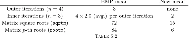
Following Bini et al. [4], we then focused on the second data set (ammonium dihydrogen phosphate) for a deeper analysis; we report in Table 5 the number of iterations and matrix roots needed in both computations.
[image:15.612.75.398.280.345.2]Outer iterations (n= 4) 4 none Inner iterations (n= 3) 4×2.5 (avg.) per outer iteration 3
Matrix square roots (sqrtm) 120 18
[image:16.612.83.428.262.456.2]Matrixp-th roots (rootm) 136 9
Table 5.3
Number of inner and outer iterations needed, and number of matrix roots needed
Operation Result
GBMP(M
−2, M, M2, M3)−M
2 4.0E-14
GN EW(M
−2, M, M2, M3)−M
2 2.5E-14
det(GBMP(A, B, C, D))−(det(A) det(B) det(C) det(D))1/4
5.5E-13
det(GBMP(A, B, C, D))−(det(A) det(B) det(C) det(D))1/4
2.1E-13 Table 5.4
Accuracy tests
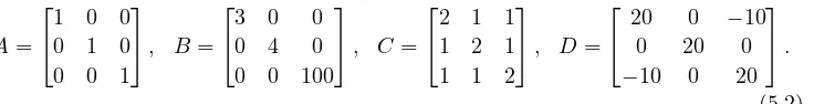
mutual distances are larger:
A=
1 0 0
0 1 0
0 0 1
, B=
3 0 0
0 4 0
0 0 100
, C=
2 1 1
1 2 1
1 1 2
, D=
20 0 −10
0 20 0
−10 0 20
.
(5.2) The results regarding these matrices are reported in Table 5.3.
Accuracy. It is not clear how to check the accuracy of a limit process yielding a matrix geometric mean, since the exact value of the mean is not known a priori, apart from the cases in which all theAicommute. In those cases, P1 yields a compact
expression for the result. So we cannot test accuracy in the general case; instead, we have focused on two special examples.
As a first accuracy experiment, we computed G(M−2, M, M2, M3)−M, where
[image:16.612.77.445.403.450.2]6. Conclusions.
Research lines. The results of this paper show that, by combining existing matrix means, it is possible to create a new mean which is faster to compute than the existing ones. Moreover, we show that using only function compositions and limit processes with the existing proof strategies, it is not possible to achieve any further significant improvement with respect to the existing algorithms. In particular, the dependency fromn! cannot be removed. New attempts should focus on other aspects, such as:
• proving new “unexpected” algebraic relations involving the existing matrix means, which would allow to break out of the framework of Theorem 3.5– Theorem 4.1.
• introducing new kinds of matrix geometric means or quasi-means, different from the ones built using function composition and limits.
• proving that the Riemannian centroid (1.1) is a matrix mean in the sense of Ando–Li–Mathias (currently P4 is an open problem), or providing faster and reliable algorithms to compute it.
It is an interesting question whether it is possible to construct a quasi-mean whose isotropy group is exactlyAn.
Acknowledgments. The author would like to thank Dario Bini and Bruno Iannazzo for enlightening discussions on the topic of matrix means, and Roberto Dvornicich and Francesco Veneziano for their help with the group theory involved in the analysis of the problem.
REFERENCES
[1] T. Ando, Chi-Kwong Li, and Roy Mathias. Geometric means. Linear Algebra Appl., 385:305–334, 2004.
[2] Rajendra Bhatia.Positive definite matrices. Princeton Series in Applied Mathematics. Princeton University Press, Princeton, NJ, 2007.
[3] Rajendra Bhatia and John Holbrook. Riemannian geometry and matrix geometric means.Linear Algebra Appl., 413(2-3):594–618, 2006.
[4] Dario A. Bini, Beatrice Meini, and Federico Poloni. An effective matrix geometric mean satisfying the Ando-Li-Mathias properties. Math Comp., 2009. In press.
[5] John D. Dixon and Brian Mortimer. Permutation groups, volume 163 ofGraduate Texts in Mathematics. Springer-Verlag, New York, 1996.
[6] Yongdo Lim. On Ando-Li-Mathias geometric mean equations. Linear Algebra Appl., 428(8-9):1767–1777, 2008.
[7] Maher Moakher. A differential geometric approach to the geometric mean of symmetric positive-definite matrices. SIAM J. Matrix Anal. Appl., 26(3):735–747 (electronic), 2005.
[8] Maher Moakher. On the averaging of symmetric positive-definite tensors. J. Elasticity, 82(3):273–296, 2006.