PERTURBATION OF PURELY IMAGINARY EIGENVALUES OF HAMILTONIAN MATRICES UNDER STRUCTURED
PERTURBATIONS∗
VOLKER MEHRMANN† AND HONGGUO XU‡
Abstract. The perturbation theory for purely imaginary eigenvaluesof Hamiltonian matrices under Hamiltonian and non-Hamiltonian perturbations is discussed. It is shown that there is a substantial difference in the behavior under these perturbations. The perturbation of real eigenvalues of real skew-Hamiltonian matrices under structured perturbations is discussed as well and these results are used to analyze the properties of the URV method for computing the eigenvalues of Hamiltonian matrices.
Key words. Hamiltonian matrix, Skew-Hamiltonian matrix, Symplectic matrix, Structured perturbation, Invariant subspace, Purely imaginary eigenvalues, Passive system, Robust control, Gyroscopic system.
AMS subject classifications.15A18, 15A57, 65F15, 65F35.
1. Introduction. In this paper, we discuss the perturbation theory for
eigen-values of Hamiltonian matrices. Let F denote the real or complex field and let ∗
denote the conjugate transpose ifF=Cand the transpose ifF=R. Let furthermore,
Jn =
0 −In
In
0
. A matrixH ∈F2n,2n is calledHamiltonianif (J
nH)∗=JnH.
The spectrum of a Hamiltonian matrix has so-called Hamiltonian symmetry, i.e.,
the eigenvalues appear in (λ,−¯λ) pairs ifF=C, and in quadruples (λ,−λ,λ,¯ −λ¯) if
F=R.
When a given Hamiltonian matrix is perturbed to another Hamiltonian matrix, then in general the eigenvalues will change but still have the same symmetry pattern. If the perturbation is unstructured, then the perturbed eigenvalues will have lost this property.
∗Received by the editorsSeptember 30, 2007. Accepted for publication April 17, 2008. Handling
Editor: Harm Bart.
†Institut f¨ur Mathematik, TU Berlin, Str. des17. Juni 136, D-10623 Berlin, FRG
([email protected]). Partially supported byDeutsche Forschungsgemeinschaft, through the DFG Research CenterMatheonMathematics for Key Technologiesin Berlin.
‡Department of Mathematics, University of Kansas, Lawrence, KS 44045, USA. Partially
sup-ported bythe University of Kansas General Research Fund allocation # 2301717and byDeutsche Forschungsgemeinschaftthrough the DFG Research CenterMatheonMathematics for key technolo-giesin Berlin. Part of the work was done while this author was visiting TU Berlin whose hospitality isgratefully acknowledged.
The solution of the Hamiltonian eigenvalue problem is a key building block in many computational methods in control, see e.g., [1, 18, 31, 36, 50] and the references therein. It has also other important applications, consider the following examples.
Example 1.1. Hamiltonian matrices from robust control. In the optimal H∞
control problem one has to deal with parameterized real Hamiltonian matrices of the form
H(γ) =
F G1−γ−2G2
H −FT
,
whereF, G1, G2, H∈Rn,n,G1, G2, Hare symmetric positive semi-definite, andγ >0
is a parameter, see e.g., [16, 27, 47, 50]. In theγ iteration, one has to determine the
smallest possibleγ such that the Hamiltonian matrixH(γ) has no purely imaginary
eigenvalues and it is essential that thisγis computed accurately, because the optimal
controller is implemented with thisγ.
Example 1.2. Linear second order gyroscopic systems. The stability of linear second order gyroscopic systems, see [21, 26, 46], can be analyzed via the following quadratic eigenvalue problem
P(λ)x= (λ2I+λ(2δG)−K)x= 0,
(1.1)
whereG, K∈Cn,n,Kis Hermitian positive definite,Gis nonsingular skew-Hermitian,
andδ >0 is a parameter. To stabilize the system, one needs to find the smallest real
δ such that all the eigenvalues ofP(λ) are purely imaginary, which means that the
gyroscopic system is stable.
The quadratic eigenvalue problem (1.1) can be reformulated as the linear Hamil-tonian eigenvalue problem
(λI− H(δ))
(λI+δG)x
x
= 0, withH(δ) =
−δG K+δ2G2
In −δG
,
i.e., the stabilization problem is equivalent to determining the smallest δ such that
all the eigenvalues ofH(δ) are purely imaginary.
Athird application arises in the context of making non-passive dynamical systems passive.
Example 1.3. Dissipativity, passivity, contractivity of linear systems. Consider a control system
˙
x=Ax+Bu, x(0) =x0,
y=Cx+Du,
with real or complex matricesA∈Fn,n,B∈Fn,m,C∈Fp,n,D∈Fp,m, and suppose
that the homogeneous system is asymptotically stable, i.e., all eigenvalues ofAare in
the open left half complex plane. Assume furthermore thatD has full column rank.
Defining as in [1] a real scalar valuedsupply function s(u, y), the system is called
dissipative if there exists a nonnegative scalar valued function Θ, such that the dissi-pation inequality
Θ(x(t1))−Θ(x(t0))≤
t1
t0
s(u(t), y(t))dt
holds for allt1≥t0, i.e., the system absorbs supply energy. Adissipative system with
the supply functions(x, y) =u2− y2 is called contractive and with the supply
functions(x, y) =u∗
y+y∗
uit is calledpassive.
Setting Y = S∗
+QD, X =R+S∗
D+D∗ S+D∗
QD, it is possible to check
dissipativity, contractivity, passivity by checking, whether the Hamiltonian matrix
H=
A−BX−1Y∗
C −BX−1BT −CT(Q
−Y X−1Y∗
)−1C
−(A−BX−1Y∗ C)∗
(1.3)
has no purely imaginary eigenvalues, where in the passive caseQ= 0, R= 0, S=I
and in the contractive caseQ=−I, R=I, S= 0. It is an important task in
appli-cations from power systems [7, 19, 41] to perturb a system that is not dissipative, not contractive, or not passive, to become dissipative, contractive, passive, respectively,
by small perturbations toA, B, C, D[7, 11, 17, 41, 42], i.e., we need to construct small
perturbations that move the eigenvalues of the Hamiltonian matrix off the imaginary axis.
In all these applications, the location of the eigenvalues (in particular, of the purely imaginary eigenvalues) of Hamiltonian matrices needs to be checked numeri-cally at different values of parameters or perturbations. Using backward error analysis [20, 48], in finite precision arithmetic, the computed eigenvalues may be considered as the exact eigenvalues of a matrix slightly perturbed from the Hamiltonian matrix.
makes a fundamental difference in the decision process needed in the above discussed applications.
In recent years, a lot of effort has gone into the construction of structure preserv-ing numerical methods to compute eigenvalues, invariant subspaces and structured Schur forms for Hamiltonian matrices. Examples of such methods are the symplectic URV methods developed in [2, 3] for computing the eigenvalues of a real Hamiltonian matrix and their extension for computing the Hamiltonian Schur form [6]. These methods produce eigenvalues and Schur forms, respectively, of a perturbed Hamilto-nian matrix. To complete the evaluation of structure preserving numerical methods in finite precision arithmetic it is then necessary to carry out a structured perturbation analysis to characterize the sensitivity of the problem under structured perturbations.
This topic has recently received a lot of attention [5, 8, 22, 23, 24, 25, 30, 45]. Surprisingly, the results in several of these papers show that the structured condition numbers for eigenvalues and invariant subspaces are often the same (or only slightly
different by a factor of√2) as those under unstructured perturbations.
These observations have led to the question, whether the substantial effort that is needed to construct and implement structure preserving methods is worthwhile. How-ever, as we will show in this paper, and this is in line with previous work [10, 37, 38, 39], there is a substantial difference between the structured and unstructured perturba-tion results, in particular, in the perturbaperturba-tion of purely imaginary eigenvalues. Let us demonstrate this with an example.
Example 1.4. Consider the following Hamiltonian matrixHand the
perturba-tion matrixE given by
H=
The matrixHhas two purely imaginary eigenvaluesλ1,2=±iand the perturbed
matrix
The difference between the exact and perturbed eigenvalues is given by
so, no matter how small the perturbationEwill be, in general, the eigenvalues will move away from the imaginary axis.
However, if E is Hamiltonian, thend=−¯a andc, b are real. In this case, both
eigenvalues ˜λ1,2 are still purely imaginary when (1 +b)(1−c)−(Rea)2 ≥0, which
holds when||E||is small.
This example shows the different behavior of purely imaginary eigenvalues under Hamiltonian and non-Hamiltonian perturbations. We will analyze the reason for this difference and show that it is the existence of further invariants under structure preserving similarity transformations that are associated with these eigenvalues.
The paper is organized as follows. In Section 2, we recall some eigenvalue prop-erties for Hamiltonian matrices. In Section 3, we describe the behavior of purely imaginary eigenvalues of Hamiltonian matrices under Hamiltonian perturbations. In Section 4, we study the behavior of real eigenvalues of skew-Hamiltonian matrices with skew-Hamiltonian perturbations. In Section 5, we then derive conditions so that the symplectic URV algorithm proposed in [3] can correctly compute the purely imag-inary eigenvalues of a real Hamiltonian matrix. We finish with some conclusions in Section 6.
2. Notation and preliminaries. The subspace spanned by the columns of
matrixXis denoted by spanX. In(or simplyI) is the identity matrix. The spectrum
of a square matrixAis denoted byλ(A). The spectrum of a matrix pencilλE−Ais
denoted byλ(E, A). || · ||denotes a vector norm or a matrix norm.
We use the notationa=O(b) to indicate that|a/b| ≤Cfor some positive constant
C asb→0, and the notationa=o(b) to indicate that|a/b| →0 asb→0.
Definition 2.1. For a matrix A ∈ Fn,n, a subspace V ⊆ Fn is a right (left)
invariant subspace of A if AV ⊆ V (A∗
V ⊆ V). Let λ be an eigenvalue of A. A
right invariant subspace V of A is the right (left) eigenspace corresponding to λ if
A|V(A∗|V), the restriction ofA to V, has the single eigenvalueλ, and dimV equals
the algebraic multiplicity ofλ.
Definition 2.2.
(i) AmatrixS ∈F2n,2n is called symplectic ifS∗JnS=Jn.
(ii) AmatrixU ∈C2n,2n(R2n,2n) is calledunitary (orthogonal) symplectic if
U is
symplectic andU∗
U =I2n.
iii) AmatrixH ∈F2n,2n is calledHamiltonian ifHJn= (HJn)∗.
iv) AmatrixK ∈F2n,2n is calledskew-Hamiltonian if
KJn=−(KJn)∗.
the particular matrices
For Hamiltonian and skew-Hamiltonian matrices, structured Jordan canonical forms are well known.
Theorem 2.3 ([12, 13, 28, 29, 44, 49]). For any Hamiltonian matrixH ∈C2n,2n,
there exists a nonsingular matrix X such that
X−1
HX = diag(H1, . . . , Hm) and X∗JnX = diag(Z1, . . . , Zm),
where each pair (Hj, Zj)is of one of the following forms:
(a) Hj =iNnj(αj), Zj =isjPnj, where αj ∈R andsj =±1, corresponding to
annj×nj Jordan block for the purely imaginary eigenvalue iαj.
(b) Hj =
The scalarssj in Theorem 2.3 are called thesign characteristicof the pair (H, J)
associated with the purely imaginary eigenvalues, they satisfy
sj = 0.
In the real case, the canonical form is as follows.
Theorem 2.4 ([13, 28, 29, 44]). For any Hamiltonian matrixH ∈R2n,2n, there
exists a real nonsingular matrixX such that
(a.2) Hj =
imaginary eigenvalues±iαj.
(c) Hj =
It should be noted that in the real case, we have two sets of sign characteristics
tj,sjof the pair (H, J). Note further that both in the real and complex Hamiltonian
cases, the transformation matrixX can be constructed to be a symplectic matrix, see
[29].
For complex skew-Hamiltonian matrices, the canonical form is similar to the
Hamiltonian canonical form, since ifK is skew-Hamiltonian then iK is Hamiltonian.
For real skew-Hamiltonian matrices, the canonical form is different but simpler.
Theorem 2.5 ([9, 44]). For any skew Hamiltonian matrix K ∈ R2n,2n, there
exists a real symplectic matrixS such that
S−1KS=
whereK is in real Jordan canonical form.
Theorem 2.5 shows that every Jordan block of K appears twice, and thus, the
algebraic and geometric multiplicity of every eigenvalue must be even.
After introducing some notation and recalling the canonical forms, in the next section, we study the perturbation of purely imaginary eigenvalues of Hamiltonian matrices.
3. Perturbations of purely imaginary eigenvalues of Hamiltonian ma-trices. LetH ∈ C2n,2n be Hamiltonian and suppose that iαis a purely imaginary
the right eigenspace associated withiα, i.e.,
HX =XR,
(3.1)
whereλ(R) ={iα}. By using the Hamiltonian propertyH=−JH∗J∗, we also have
X∗
JH=−R∗ X∗
J.
(3.2)
Since alsoλ(−R∗) =
{iα}, it follows that the columns of the full column rank matrix
J∗
X span the left eigenspace ofiα. Hence, we have that
(J∗ X)∗
X =X∗ JX
is nonsingular. Then the matrix
Z :=iX∗ JX
(3.3)
is Hermitian and nonsingular. The matrix
M :=X∗(JH)X
(3.4)
is also Hermitian. Thus, by pre-multiplyingX∗
J to (3.1), we obtain
M =Z(−iR)⇒ −iR=Z−1M.
(3.5)
This implies that the spectrum of the pencilλZ−M is given by
λ(Z, M) =λ(−iR) ={α}.
We combine these observations in the following lemma.
Lemma 3.1. Let H ∈ C2n,2n be Hamiltonian and suppose that iα is a purely
imaginary eigenvalue of H. Let R, X, Z be as defined in (3.1) and (3.3). Then the matrixZ is definite if and only ifiαis a multiple eigenvalue with equal algebraic and geometric multiplicity and has uniform sign characteristic.
Proof. Since the Sylvester inertia index ofZ, i.e., the number of positive, negative or zero eigenvalues, is independent of the choice of basis, based on the structured
canonical form in Theorem 2.3 (a), we may chooseX such that
R= diag(iNn1(α), . . . , iNnq(α)) and Z=−diag(s1Pn1, . . . , spPnq),
(3.6)
wheresj =±1 are the corresponding sign characteristics.
Ifnj >1 for somej, thenZ has a diagonal block−sjPnj which is indefinite, and
thus, Z is indefinite. If n1=· · ·=nq = 1, thenZ =−diag(s1, . . . , sq) so that Z is
With the help of Lemma 3.1 we can now characterize the behavior of purely imag-inary eigenvalues under Hamiltonian perturbations. This topic is well studied in the more general context of self-adjoint matrices with respect to indefinite inner products, see [14, 15]. Adetailed perturbation analysis of the sign characteristics is given in [40] for the case that the Jordan structure is kept fixed as well as the multiplicities of nearby eigenvalues. We are, in particular, interested in the purely imaginary eigen-values of Hamiltonian matrices and to characterize how many eigeneigen-values stay on the imaginary axis and how many move away from the axis. This cannot be concluded directly from these results, so we present a different analysis and proof.
Theorem 3.2. Consider a Hamiltonian matrix H ∈C2n,2n with a purely
imag-inary eigenvalue iα of algebraic multiplicity p. Suppose that X ∈ C2n,p satisfies
rankX =pand (3.1), and that Z andM are defined as in (3.3) and (3.4), whereZ
is congruent toIπ
0 0
−Iµ
(with π+µ=p).
If E is Hamiltonian and||E|| is sufficiently small, then H+E has p eigenvalues
λ1, . . . , λp (counting multiplicity) in the neighborhood ofiα, among which at least|π−
µ|eigenvalues are purely imaginary. In particular, we have the following possibilities. 1. If Z is definite, i.e., either π = 0 or µ = 0, then all λ1, . . . , λp are purely
imaginary with equal algebraic and geometric multiplicity, and satisfy
λj =i(α+δj) +O(||E||2),
whereδ1, . . . , δp are the real eigenvalues of the pencilλZ−X∗(JE)X.
2. If there exists a Jordan block associated with iα of size larger than 2, then generically for a givenE, some eigenvalues ofH+E will no longer be purely imaginary.
If there exists a Jordan block associated withiαof size2, then for any ǫ >0, there always exists a Hamiltonian perturbation matrix E with ||E|| = ǫ such that some eigenvalues of H+E will have nonzero real part.
3. If iαhas equal algebraic and geometric multiplicity andZ is indefinite, then for any ǫ >0, there always exists a Hamiltonian perturbation matrix E with
||E||=ǫsuch that some eigenvalues of H+E will have nonzero real part. Proof. We first prove the general result and then turn to the three special cases. Consider the Hamiltonian matrix
H(t) =H+tE,
with 0 ≤t≤ 1. If ||E||is sufficiently small, then by the classical invariant subspace
perturbation theory [43], there exists a full column rank matrixX(t)∈C2n,p, which
is a continuous function oftsatisfyingX(0) =X such that
H(t)X(t) =X(t)R(t),
where R(t) has the eigenvalues λ1(t), . . . , λp(t). These peigenvalues satisfy λ1(0) = · · ·=λp(0) =iα, and are close toiαand separated from the rest of the eigenvalues
ofH(t) for 0< t≤1.
SinceH(t) is Hamiltonian, similarly, for
Z(t) =iX(t)∗
JX(t) and M(t) =X(t)∗
(JH(t))X(t),
we have the properties thatZ(t) is Hermitian nonsingular,M(t) is Hermitian and
λ(Z(t), M(t)) =λ(−iR(t)) ={−iλ1(t), . . . ,−iλp(t)}.
Because Z(t) is also a continuous function of t, and Z(0) = Z, detZ(t) = 0 for
0≤t≤1, we have thatZ(t) is congruent toIπ
0 0
−Iµ
, i.e.,Z(t) has the same inertia
asZfor 0≤t≤1. Therefore,Z(1) is congruent toIπ
0 0
−Iµ
. Based on the structured
canonical form of Hermitian/Hermitian pencils [32, 44], the pencilλZ(1)−M(1) has
at least |π−µ| real eigenvalues. Sinceλ(R(1)) =iλ(Z(1), M(1)), we conclude that
R(1), or equivalentlyH+E=H(1) has at least|π−µ|purely imaginary eigenvalues
neariα.
It follows from (3.1) and (3.2) that
X∗
JXR=−R∗ X∗
JX,
i.e.,
−(X∗JX)−1R∗=R(X∗JX)−1.
Then, forY = ((X∗JX)−1X∗J)∗, by (3.2), we have
Y∗
H=RY∗ ,
andY∗
X =Ip.
It follows from first order perturbation theory [43], that for||E||sufficiently small,
the eigenvaluesλ1, . . . , λp ofH+E that are close toiαare eigenvalues of
˜
R=Y∗
(H+E)X+δE,
where||δE||=O(||E||2). This relation can be written as
˜
R=R+iZ−1X∗(JE)X+δE.
(3.8)
We start to prove part 1. When Z is definite, i.e., either π = 0 or µ = 0,
definite. Therefore, since |π−µ| = p, H+E has p purely imaginary eigenvalues
λ1:=λ1(1), . . . , λp:=λp(1).
When Z is definite, then the Hermitian pencil λZ−X∗
(JE)X as well as the
matrix Z−1X∗(J
E)X have real eigenvalues δ1, . . . , δp. By Lemma 3.1, when Z is
definite, it follows thatR=iαI. Thus by (3.8), for the eigenvalues of the perturbed
problem we have
λj =iα+iδj+O(||E||2),
forj= 1, . . . , p.
We now prove the first part of part 2. The second part will be given in Example 3.4
below. Without loss of generality, we assume that R and Z are given as in (3.6),
where nj >1 for some j. Note that (3.8) still holds. Generically, for unstructured
perturbations, the largest eigenvalue perturbation occurs in the largest Jordan blocks, see [33, 34] and for generic structured perturbations of Hamiltonian matrices this is
true as well [25]. Thus, for simplicity of presentation, we assume thatRconsists ofq
equal blocks of sizer:=n1=· · ·=nq >1. (Otherwise, we could first only consider
the perturbation of the submatrix associated with the largest Jordan blocks.) Then
with an appropriate permutationP,R andZ can be simultaneously transformed to
R1=PTRP andZ1=PTZP with
Then ˜R1 has at leastrteigenvalues that can be expressed as
iα+iρk,j+o(||E||
1
r)
Clearly, if r > 2, then in general there always exist some non-real ρk,j, which
implies that ˜R1 and, therefore, alsoH+E have some eigenvalues nearbyiαbut with
nonzero real parts.
In this case, the eigenvalues of ˜Rcan be expressed as
λj =iα+ρj+O(||E||2),
where ρ1, . . . , ρp are the eigenvalues ofiZ−1X∗(JE)X, or equivalently, the
Hermiti-an/skew-Hermitian pencil
λZ−iX∗
(JE)X.
Since Z is indefinite, one can always find E, no matter how small ||E||is, such that
this pencil has eigenvalues with nonzero real part and thus alsoλj must have nonzero
real part.
Remark 3.3. The eigenvaluesδ1, . . . , δp in the first order perturbation formula
are independent of the choice of the subspace X. If Y is a full column rank matrix
such that spanY = spanX, thenY =XT for some nonsingular matrixT. Therefore,
λiY∗
associatedZ is the reciprocal of the condition number of iα.
In the following we give two examples to illustrate parts 2 and 3 in Theorem 3.2.
Example 3.4. Suppose thatHconsists of only one 2×2 Jordan block associated
with the purely imaginary eigenvalueiα, and letX be a full column rank matrix such
that
is Hermitian). Then the eigenvalues of ˜R
are
λ1,2=i
No matter how small||E||is, we can always findE with (Imb)2+a(s−c)>0. Then
bothλ1, λ2 have nonzero real part.
Theorem 3.2 can now be used to explain why the purely imaginary eigenvalues
±iof the Hamiltonian matrixHin Example 1.4 are hard to move off the imaginary
axis by Hamiltonian perturbations. The reason is that if we take the eigenvectors of
iand −i as 1 i
and−1i
, respectively, the corresponding matrices Z are−2 and 2,
respectively, which are both definite.
Let us consider another example.
Example 3.5. The Hamiltonian matrices
H1=
both have a pair of purely imaginary eigenvalues±iwith algebraic multiplicity 2. For
the eigenvaluei, the right eigenspaces are spanned by the columns of the matrices
X1=
and the correspondingZ matrices are
Z1= 2i
respectively. ForH1, a small Hamiltonian perturbation may moveioff the imaginary
axis, while forH2, only a large Hamiltonian perturbation can achieve this.
For an eigenvalue of a Hamiltonian matrix that is not purely imaginary, based on the Hamiltonian canonical form, it is not difficult to show that a general Hamiltonian perturbation (regardless of the perturbation magnitude) is very unlikely to move the eigenvalue to the imaginary axis. If one really wants to construct a perturbation that moves an eigenvalue with nonzero real part to the imaginary axis, then one needs to construct special perturbation matrices [35].
In the context of the passivation problem in Example 1.3 one has to study the
problem, what is the minimal norm of a Hamiltonian perturbationE that is needed
the case that all the purely imaginary eigenvalues are as in part 1 of Theorem 3.2. We then have the following result.
Theorem 3.6. Suppose that H ∈C2n,2n is Hamiltonian and all its eigenvalues
are purely imaginary. Let H2n be the set of 2n×2n complexHamiltonian matrices,
and letS be the set of Hamiltonian matrices defined by S=
E ∈H2n | H+E has an imaginary eigenvalue with algebraic
multiplicity >1 and the correspondingZ in (3.3) is indefinite
.
Define
µ0= min
E ∈S||E||.
If every eigenvalue of Hhas equal algebraic and geometric multiplicity and the cor-responding matrix Z as in (3.3) is definite, then for any Hamiltonian matrix E with
||E|| ≤µ0,H+E has only purely imaginary eigenvalues. For anyµ > µ0, there always
exists a Hamiltonian matrixE with ||E||=µsuch that H+E has an eigenvalue with nonzero real part.
Proof. By the assumption, we may divide the purely imaginary eigenvalues into
ksetsL1, . . . , Lk such that
(i) for i < j, any eigenvalue λi,ℓ ∈Li is below all the eigenvaluesλj,ℓ ∈ Lj on
the imaginary axis,
(ii) the eigenvaluesλi,ℓ in each setLi have the corresponding matricesZi,ℓas in
(3.3) either all positive definite or all negative definite, and
(iii) the definiteness is alternating on the sets, i.e., if theZj,ℓ associated with the
setLj are all positive definite, then they are all negative definite onLj+1.
For the eigenvalues in set Lj, we define the full column rank matrix Xj such that
the columns of Xj span the corresponding invariant subspace. Also we defineZj =
iX∗
jJXj forj= 1, . . . , k.
Because in the set Lj, for all the eigenvalues, the corresponding matrices Zj,ℓ
have the same definiteness, Zj is also definite and the definiteness alternates from
positive to negative.
Now let E be a Hamiltonian perturbation. Then the eigenvalues of H+E are
continuous functions of the entries ofE. By using the continuity argument as for case
1 of Theorem 3.2, it follows that the eigenvalues ofH+Eare all purely imaginary and
in k separated sets L1(E), . . . , Lk(E), regardless of their algebraic multiplicity, until
for some E two neighboring eigenvalue sets have a common element. The common
element is an eigenvalue ofH+Eand the associated matrixZmust be indefinite, since
any small Hamiltonian perturbation may move this eigenvalue off the imaginary axis.
Using the Hamiltonian canonical form, one can always find such a perturbationE. So
the minimization problem has a well-defined minimum.
IfHalso has some eigenvalues that are not purely imaginary, then the situation is
much more complicated, and in general, Theorem 3.6 does not hold. The complexity of the problem in this case can be illustrated by the following example.
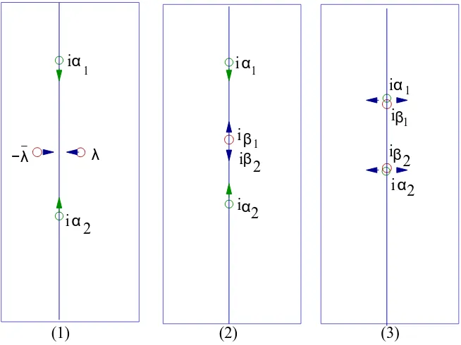
Example 3.7. Consider a 4×4 Hamiltonian matrixHwith two purely imaginary
eigenvalues iα1, iα2 and eigenvaluesλ,−λ¯, with nonzero real part, see Figure 3.1. If
α
β
β
β
i
i
i
(1)
(2)
(3)
α
1
i
−λ
λ
2
i
α
α
i
i
i
β
α
i
i
α
2
2
2
2
1
1
1
1
Fig. 3.1.Eigenvalue perturbations in Example 3.7
we consider the perturbationE to moveiα1, iα2 off the imaginary axis, while freezing
λ,−λ¯, then we basically obtain the same result as in Theorem 3.6 with an additional
restriction to E. However, the involvement of λ,−λ¯ may help to reduce the norm
of E to move off iα1, iα2. Suppose that λ,−λ¯ are already close to the imaginary
axis as in Figure 3.1 (1). We may construct first a small perturbation that moves
λ,−λ¯ to the imaginary axis, forming a double purely imaginary eigenvaluesiβ1, iβ2
and by continuity it follows that its associated matrix Z is indefinite. Meanwhile,
we also move iα1, iα2 towards each other with an appropriate perturbation. Next
we determine another perturbation that forcesiβ1, iβ2to move in opposite direction
we force theZ matrices (they are scalar in this case) associated withiαj, iβj to have
opposite signs forj = 1,2. When iα1, iβ1 andiα2, iβ2 meet, they will be moved off
the imaginary axis, see Figure 3.1 (3). It is then possible to have anE with a norm
smaller than the one that freezesλ,−¯λ.
To make this concrete, consider the Hamiltonian matrix
H=
2. ThenH has two purely imaginary eigenvaluesi, −iand two real
eigenvaluesµ,−µ. The Hamiltonian matrices of the form
E1=
with b, c ∈ Ronly perturb the eigenvalues i and −i. Using the eigenvalue formula
obtained in Example 1.4 and some elementary analysis, the minimum 2-norm ofE1
for bothiand−ito move to 0 is 1 (say, witha= 0,b= 0 andc= 1). Then a random
Hamiltonian perturbation with an arbitrary small 2-norm will move the eigenvalues off the imaginary axis.
On the other hand, for the Hamiltonian perturbation
E2=
This matrix has a pair of purely imaginary eigenvalues±i
2 with algebraic multiplicity
2. One can easily verify that for both i
2 and − i
2, the corresponding matrix Z is
indefinite. Then a random Hamiltonian perturbation with an arbitrary small 2-norm will move the eigenvalues off the imaginary axis. Note that
||E2||2=
1
This example also demonstrates that the problem discussed in Example 1.3 of computing a minimum norm Hamiltonian perturbation that moves all purely imag-inary eigenvalues of a Hamiltonian matrix from the imagimag-inary axis is even more difficult. To achieve this it may be necessary to use a pseudo-spectral approach as suggested in [22].
Remark 3.8. So far we have studied complex Hamiltonian matrices and complex
perturbations. For a real Hamiltonian matrixHand real Hamiltonian perturbations,
we know that the eigenvalues occur in conjugate pairs. Then if iα (α = 0) is an
eigenvalue ofH, so is−iα, and from the real Hamiltonian Jordan form in Theorem 2.4
it follows that both eigenvalues have the same properties. Thus, in the real case, one only needs to focus on the purely imaginary eigenvalues in the top half of the imaginary axis. It is not difficult to get essentially the same results as in Theorems 3.2 and 3.6 for these purely imaginary eigenvalues.
The only case that needs to be studied separately is the eigenvalue 0. By
The-orem 2.4 (a), if 0 is an eigenvalue ofH, then it has either even-sized Jordan blocks,
or pairs of odd-sized Jordan blocks with correspondingZ indefinite, or both. This is
the situation as in parts 2 and 3 of Theorem 3.2. So we conclude that 0 is a sensi-tive eigenvalue, meaning that a real Hamiltonian perturbation with arbitrary small norm will move the eigenvalue out of the origin, and there is no guarantee that the perturbed eigenvalues will be on the real or imaginary axis.
4. Perturbation of real eigenvalues of skew-Hamiltonian matrices. IfK
is a complex skew-Hamiltonian matrix, then iK is a complex Hamiltonian matrix.
So the real eigenvalues of K under skew-Hamiltonian perturbations behave in the
same way as the purely imaginary eigenvalues ofiKunder Hamiltonian perturbations.
Theorems 3.2 and 3.6 can be simply modified forK.
IfK is real and we consider real skew-Hamiltonian perturbations, then the
situ-ation is different. The real skew-Hamiltonian canonical form in Theorem 2.5 shows that each Jordan block occurs twice and the algebraic multiplicity of every eigenvalue is even. We obtain the following perturbation result.
Theorem 4.1. Consider the skew-Hamiltonian matrix K ∈ R2n,2n with a real
eigenvalueαof algebraic multiplicity 2p.
1. If p= 1, then for any skew-Hamiltonian matrix E ∈R2n,2n with sufficiently
small||E||,K+E has a real eigenvalueλclose toαwith algebraic and geometric multiplicity 2, which has the form
where η is the real double eigenvalue of the2×2 matrixpencil λXTJ nX−
XT(J
nE)X, and X is a full column rank matrixso that the columns of X
span the right eigenspace associated with α.
2. If there exists a Jordan block associated with α of size larger than 2, then generically for a givenE some eigenvalues ofK+E will no longer be real. If there exists a Jordan block associated withαof size2, then for any ǫ >0, there always exists an E with ||E|| =ǫ such that some eigenvalues ofK+E
will be non-real.
3. If the algebraic and geometric multiplicities of α are equal and are greater than 2, then for any ǫ >0, there always exists an E with ||E||=ǫ such that some eigenvalues ofK+E will be non-real.
Proof. Based on the real skew-Hamiltonian canonical form in Proposition 2.5, we
may determine a full column rank real matrix X ∈ R2n,2p such that spanX is the
eigenspace corresponding toαand
XTJnX =Jp, KX =XR, λ(R) ={α}.
If||E||is sufficiently small, then for the perturbed matrix ˜K=K+Eand the associated ˜
X and ˜Rsuch that (K+E) ˜X = ˜XR˜, we have that
||X˜ −X||=O(||E||), X˜TJ
nX˜ =Jp,
where all the eigenvalues of ˜R are close toα. This implies that
˜
XTJn(K+E) ˜X =JpR,˜
(4.1)
and as in the Hamiltonian case we have the first order perturbation expression for ˜R
given by
˜
R=R+JpTX T
(JnE)X+δE,
(4.2)
with||δE||=O(||E||2).
We now prove part 1. When p= 1, then since the left hand side of (4.1) is real
skew-symmetric, we have
˜
R=λI2,
whereλis real. Clearlyλis a real eigenvalue ofK+E and by assumption it is close
toα. Soλhas algebraic and geometric multiplicity 2 when||E||is sufficiently small.
SinceXT(J
nE)X is real skew-symmetric andp= 1 it follows that
JT pX
T(J
where η is real, Obviously η is an eigenvalue of λJp−XT(JnE)X with algebraic
and geometric multiplicity 2. Note that the eigenvalues of λJp −XT(JnE)X are
independent of the choice ofX.
Using (4.2), parts 2 and 3 can be proved in the same way as the corresponding parts of Theorem 3.2.
5. Perturbation theory for the symplectic URV algorithm. In this sec-tion, we will make use of the perturbation results obtained in Section 4 to analyze the perturbation of eigenvalues of real Hamiltonian matrices computed by the symplectic URV method proposed in [3].
For a real Hamiltonian matrix H, the symplectic URV method computes the
factorization
UTHV=R=
R1 R3
0 RT
2
,
(5.1)
where U,V are real orthogonal symplectic, R1 is upper triangular, and R2 is
quasi-upper triangular. Then, sinceHis Hamiltonian, there exists another factorization
VTHU=JRTJ =
−R2 RT3
0 −RT
1
.
(5.2)
Combining (5.1) and (5.2), we see that
UTH2U =
−R1R2 R1RT3 −R3RT1
0 −(R1R2)T
.
The matrixH2 is real skew-Hamiltonian and its eigenvalues are the same as those of
−R1R2 but with double algebraic multiplicity. Note that the eigenvalues of −R1R2
can be simply computed from its diagonal blocks. Ifγ is an eigenvalue ofH2, then
±√γ are both eigenvalues ofH.
In [3], the following backward error analysis was performed. Let ˆR be the
fi-nite precision arithmetic result when computing R in (5.1). Then there exist real
orthogonal symplectic matrices ˆU and ˆV such that
ˆ
UT(
H+F) ˆV= ˆR,
(5.3)
whereFis a real matrix satisfying||F||=c||H||ε, with a constantcandεthe machine
precision.
Similarly, there exists another factorization
ˆ
VT(
H+JFTJ) ˆ
Thus, one has
ˆ
UT(
H2+E) ˆU = ˆRJRˆTJ,
where
E=JT[(J
FH −(JFH)T)
−(JF)J(JF)T],
(5.4)
is real skew-Hamiltonian. So the computed eigenvalues that are determined from the
diagonal blocks of ˆRJRˆTJare the exact eigenvalues ofH2+E, which is the real
skew-Hamiltonian matrixH2 perturbed by a small real skew-Hamiltonian perturbation
E. We then obtain the following perturbation result.
Theorem 5.1. Suppose that λ=iα (α = 0) is a purely imaginary eigenvalue of a real Hamiltonian matrix Hand suppose that we compute an approximation ˆλby the URV method with backward errorsE andF as in (5.4) and (5.3), respectively.
1. If λ = iα is simple, and ||F|| is sufficiently small, then the URV method yields a computed eigenvalue ˆλ=iαˆ near λ, which is also simple and purely imaginary. Moreover, letX be a real and full column rank matrixsuch that
HX =X
0 α
−α 0
and XTJ
nX=J1,
and let
XTJ FX =
f11 f12
f21 f22
.
Then
iαˆ−iα=−if11+f22
2 +O(||F||
2).
2. Ifλ=iαis not simple orλ= 0, then the corresponding computed eigenvalue may not be purely imaginary.
Proof. Ifiαis a nonzero purely imaginary eigenvalue ofH, then so is−iα. Thus
−α2 is a negative eigenvalue ofH2 with algebraic and geometric multiplicity 2. Let
ˆ
µ be the computed eigenvalue of H2 that is close to µ =
−α2. Then ˆµ is also an
eigenvalue ofH2+
E.
For part 1, if ||F||is sufficiently small, then by part 1 of Theorem 4.1, ˆµ is real
and negative. Thus, we can express ˆµ as ˆµ= −αˆ2 and ˆαhas the same sign as α.
Note that
and||E||=O(||F||). Thus, by Theorem 4.1, we have
−αˆ2=
−α2+η+O( ||F||2),
whereη is the double real eigenvalue of
λJ1−XT(JE)X.
Using (5.4) and thatHX =αXJ1, we obtain
XT(JE)X =αXTJFXJ1−αJ1TX T
FTJTX+XTFJFTJTX
=α(XTJFXJ1−J1TX
T
FTJTX) +XTFJFTJTX
=α(f11+f12)J1+XTFJFTJTX,
which implies that
η=α(f11+f12) +O(||F||2).
Then we have that
−αˆ2+α2=α(f
11+f22) +O(||F||2),
and thus,
ˆ
α−α=−αˆ+αα(f11+f22) +O(||F||2),
which can be expressed as
iαˆ−iα=−if11+f22
2 +O(||F||
2).
In part 2, ifiαis not simple andα= 0, then−α2is an eigenvalue of
H2with algebraic
multiplicity greater than 2. By parts 2 and 3 of Theorem 4.1, we cannot guarantee
that the computed eigenvalue is still purely imaginary. Ifα= 0 then by Remark 3.8,
again there is no guarantee that the computed eigenvalues will be on the real axis or imaginary axis.
Note that the first order error bound of Theorem 5.1 was already given in [3] for
simple eigenvalues ofH.
Although the symplectic URV method provides the computed spectrum ofHwith
Hamiltonian symmetry, it can well approximate the location of the nonzero simple
purely imaginary eigenvalues of H. An analysis of the behavior of the method for
multiple purely imaginary eigenvalues is an open problem.
6. Conclusion. We have presented the perturbation analysis for purely imagi-nary eigenvalues of Hamiltonian matrices under Hamiltonian perturbations. We have shown that the structured perturbation theory yields substantially different results than the unstructured perturbation theory, in that it can (in some situations) be guaranteed that purely imaginary eigenvalues stay on the imaginary axis under struc-tured perturbations while they generically move off the imaginary axis in the case of unstructured perturbations. These results show that the use of structure preserving methods can make a substantial difference in the numerical solution of some impor-tant practical problems arising in robust control, stabilization of gyroscopic systems as well as passivation of linear systems. We have also used the structured perturbation results to analyze the properties of the symplectic URV method of [3].
Acknowledgment. We thank R. A lam, S. Bora, D. Kressner, and J. Moro for fruitful discussions on structured perturbations, L. Rodman for providing further references, and L. Trefethen for initiating the discussion on the usefulness of structured perturbation analysis. We also thank an anonymous referee for helpful comments that improved the paper.
REFERENCES
[1] T. Antoulas. Approximation of Large-Scale Dynamical Systems. SIAM Publications, Philadel-phia, PA, USA, 2005.
[2] P. Benner, V. Mehrmann, and H. Xu. A new method for computing the stable invariant subspace of a real Hamiltonian matrix. J. Comput. Appl. Math., 86:17–43, 1997.
[3] P. Benner, V. Mehrmann, and H. Xu. A numerically stable, structure preserving method for computing the eigenvalues of real Hamiltonian or symplectic pencils.Numer. Math., 78:329– 358, 1998.
[4] P. Benner, V. Mehrmann, and H. Xu. A note on the numerical solution of complex Hamiltonian and skew-Hamiltonian eigenvalue problems. Electr. Trans. Num. Anal., 8:115–126, 1999. [5] R. Byers and D. Kressner. Structured condition numbers for invariant subspaces. SIAM J.
Matrix Anal. Appl., 28:326 – 347, 2006.
[6] D. Chu, X. Liu, and V. Mehrmann. A numerical method for computing the Hamiltonian Schur form. Numer. Math., 105:375–412, 2007.
[7] C.P. Coelho, J.R. Phillips, and L.M. Silveira. Robust rational function approximation algo-rithm for model generation. InProceedings of the 36th DAC, pages207–212, New Orleans, Louisiana, USA, 1999.
[8] H. Faßbender and D. Kressner. Structured eigenvalue problems. GAMM Mitteilungen, 29:297 – 318, 2006.
[9] H. Faßbender, D.S. Mackey, N. Mackey, and H. Xu. Hamiltonian square roots of
skew-Hamiltonian matrices. Linear Algebra Appl., 287:125–159, 1999.
[10] G. Freiling, V. Mehrmann, and H. Xu. Existence, uniqueness and parametrization of Lagrangian invariant subspaces. SIAM J. Matrix Anal. Appl., 23:1045–1069, 2002.
[11] R.W. Freund and F. Jarre. An extension of the positive real lemma to descriptor systems.
Optim. Methods Softw., 19:69–87, 2004.
[13] I. Gohberg, P. Lancaster, and L. Rodman. Spectral analysis of self-adjoint matrix polynomials.
Ann. of Math., 112:33–71, 1980.
[14] I. Gohberg, P. Lancaster, and L. Rodman. Perturbations ofH-selfadjoint matrices with appli-cationsto differential equations.Integral Equations Operator Theory, 5:718–757, 1982.
[15] I. Gohberg, P. Lancaster, and L. Rodman. Indefinite Linear Algebra and Applications.
Birkh¨auser, Basel, 2005.
[16] M. Green and D.J.N. Limebeer. Linear Robust Control. Prentice-Hall, Englewood Cliffs, NJ, 1995.
[17] S. Grivet-Talocia. Passivity enforcement via perturbation of Hamiltonian matrices.IEEE Trans. Circuits Systems, 51:1755–1769, 2004.
[18] D.-W. Gu, P.H. Petkov, and M.M. Konstantinov. Robust Control Design with MATLAB.
Springer-Verlag, Berlin, FRG, 2005.
[19] B. Gustavsen and A. Semlyen. Enforcing passivity for admittance matrices approximated by rational functions. IEEE Trans. on Power Systems, 16:97–104, 2001.
[20] N.J. Higham. Accuracy and Stability of Numerical Algorithms. SIAM, Philadelphia, PA, 1996. [21] R. Hryniv, W. Kliem, P. Lancaster, and C. Pommer. A precise bound for gyroscopic
stabiliza-tion. Z. Angew. Math. Mech., 80:507 – 516, 2000.
[22] M. Karow. µvalues and spectral value sets for linear perturbation classes defined by a scalar product. Preprint 406, DFG Research CenterMatheon,Mathematics for key technologies
in Berlin, TU Berlin, Str. des17. Juni 136, D-10623 Berlin, Germany, 2007.
[23] M. Karow, D. Kressner, and F. Tisseur. Structured eigenvalue condition numbers. SIAM J. Matrix Anal. Appl., 28:1052–1068, 2006.
[24] D. Kressner. Perturbation bounds for isotropic invariant subspaces of skew-Hamiltonian matri-ces. SIAM J. Matrix Anal. Appl., 26:947–961, 2005.
[25] D. Kressner, M.J. Pel´aez, and J. Moro. Structured H¨older eigenvalue condition numbersfor multiple eigenvalues. Uminf report, Department of Computing Science, Ume˚a Univers ity, Sweden, 2006.
[26] P. Lancaster. Strongly stable gyroscopic systems.Electron. J. Linear Algebra, 5:53–66, 1999. [27] P. Lancaster and L. Rodman.The Algebraic Riccati Equation. Oxford University Press, Oxford,
1995.
[28] P. Lancaster and L. Rodman. Canonical forms for symmetric/skew-symmetric real matrix pairs under strict equivalence and congruence. Linear Algebra Appl., 405:1–76, 2005.
[29] W.-W. Lin, V. Mehrmann, and H. Xu. Canonical formsfor Hamiltonian and symplectic matrices and pencils. Linear Algebra Appl., 301–303:469–533, 1999.
[30] C. Mehl, V. Mehrmann, A. Ran, and L. Rodman. Perturbation analysis of Lagrangian invariant
subspaces of symplectic matrices. Technical Report 372, DFG Research CenterMatheon
in Berlin, TU Berlin, Berlin, Germany, 2006. To appear inLinear and Multilinear Algebra.
[31] V. Mehrmann. The Autonomous Linear Quadratic Control Problem, Theory and Numerical
Solution. Number 163 in Lecture Notesin Control and Information Sciences. Springer-Verlag, Heidelberg, July 1991.
[32] V. Mehrmann and H. Xu. Structured Jordan canonical formsfor structured matricesthat are Hermitian, skew Hermitian or unitary with respect to indefinite inner products. Electron. J. Linear Algebra, 5:67–103, 1999.
[33] J. Moro, J.V. Burke, and M.L. Overton. On the Lidskii-Lyusternik-Vishik perturbation theory for eigenvalueswith arbitrary Jordan structure. SIAM J. Matrix Anal. Appl., 18:793–817, 1997.
[34] J. Moro and F.M. Dopico. Low rank perturbation of Jordan structure. SIAM J. Matrix Anal. Appl., 25:495–506, 2003.
[35] M.L. Overton and P. Van Dooren. On computing the complex passivity radius. InProc. 44th IEEE Conference on Decision and Control, pages7960–7964, Sevilla, Spain, December 2005.
Control Systems. Prentice-Hall, Hemel Hempstead, Herts, UK, 1991.
[37] A.C.M. Ran and L. Rodman. Stability of invariant maximal semidefinite subspaces. Linear Algebra Appl., 62:51–86, 1984.
[38] A.C.M. Ran and L. Rodman. Stability of invariant Lagrangian subspaces I.Oper. Theory Adv. Appl. (I. Gohberg ed.), 32:181–218, 1988.
[39] A.C.M. Ran and L. Rodman. Stability of invariant Lagrangian subspaces II.Oper. Theory Adv. Appl. (H.Dym, S. Goldberg, M.A. Kaashoek and P. Lancaster eds.), 40:391–425, 1989. [40] L. Rodman. Similarity vs unitary similarity and perturbation analysis of sign characteristics:
Complex and real indefinite inner products. Linear Algebra Appl., 416:945–1009, 2006. [41] D. Saraswat, R. Achar, and M. Nakhla. On passivity check and compensation of macromodels
from tabulated data. In7th IEEE Workshop on Signal Propagation on Interconnects, pages 25–28, Siena, Italy, 2003.
[42] C. Schr¨oder and T. Stykel. Passivation of LTI systems. Technical Report 368, DFG Research Center Matheon, Technische Universit¨at Berlin, Straße des17. Juni 136, 10623 Berlin, Germany, 2007.
[43] G.W. Stewart and J.-G. Sun.Matrix Perturbation Theory. Academic Press, New York, 1990. [44] R. C. Thompson. Pencils of complex and real symmetric and skew matrices. Linear Algebra
Appl., 147:323–371, 1991.
[45] F. Tisseur. A chart of backward errors for singly and doubly structured eigenvalue problems.
SIAM J. Matrix Anal. Appl., 24:877 – 897, 2003.
[46] F. Tisseur and K. Meerbergen. The quadratic eigenvalue problem. SIAM Rev., 43:235–286, 2001.
[47] H.L. Trentelman, A.A. Stoorvogel, and M. Hautus. Control Theory for Linear Systems.
Springer-Verlag, London, UK, 2001.
[48] J.H. Wilkinson. Rounding Errors in Algebraic Processes. Prentice-Hall, Englewood Cliffs, NJ, 1963.
[49] J. Willamson. On the algebraic problem concerning the normal form of linear dynamical systems.
Amer. J. Math., 58:141–163, 1936.