Structural Change and Economic Dynamics 11 (2000) 433 – 472
Human capital investment and economic
growth: exploring the cross-country evidence
Edward N. Wolff *
Department of Economics,Faculty of Arts and Science,New York Uni6ersity,7th Floor, 269Mercer Street,New York,NY10003-6687,USA
Received 1 October 1999; received in revised form 1 July 2000; accepted 29 August 2000
Abstract
The paper investigates three models on the role of education in economic growth: human capital theory, a threshold effect, and interaction effects between education and technological activity. Data for 24 OECD countries on GDP, employment, and investment from the Penn World Tables over the period 1950 to 1990 was used. Five sources are used for educational data. The descriptive statistics suggest that the convergence in labor productivity levels among these nations appears to correspond to their convergence in schooling levels. However, econometric results showing a positive and significant effect of formal education on productivity growth among OECD countries are spotty at best. With only one or two exceptions, educational levels, the growth in educational attainment, and interaction effects between schooling and R&D were not found to be significant determinants of country labor productivity growth. © 2000 Elsevier Science B.V. All rights reserved.
Keywords:Productivity; Convergence; Education; Human capital
www.elsevier.nl/locate/strueco
1. Introduction
There are three paradigms which appear to dominate current discussions of the role of education in economic growth: the first has stemmed from human capital theory; the second could be classified as catch-up models; and the third important approach has stressed the interactions between education and technological innova-tion and change.
* Tel.:+1-212-9988900; fax: +1-212-9954186.
E-mail address:[email protected] (E.N. Wolff).
434 E.N.Wolff/Structural Change and Economic Dynamics11 (2000) 433 – 472
1.1.The human capital approach
Human capital theory views schooling as an investment in skills and hence as a way of augmenting worker productivity (see, for example, Schultz, 1960, 1961, 1971; Becker, 1975).1 This line of reasoning leads to growth accounting models in
which productivity or output growth is derived as a function of the change in educational attainment.
The early studies on this subject showed very powerful effects of educational change on economic growth. Griliches (1970) estimated that the increased educa-tional attainment of the U.S. labor force accounted for one-third of the Solow residual, the portion of the growth of output that could not be attributed to the growth in (unadjusted) labor hours or capital stock, between 1940 and 1967. Denison (1979) estimated that about one-fifth of the growth in U.S. national income per person employed between 1948 and 1973 could be attributed to increases in educational levels of the labor force.2Jorgenson and Fraumeni (1993)
calculated that improvements in labor quality accounted for one fourth of U.S. economic growth between 1948 and 1986. Maddison (1987), in a growth accounting study of six OECD countries, covering the years 1913 – 1984 generally found that increases in educational attainment explained a significant proportion of productiv-ity growth, though the contributions varied by country and sub-period.
Yet, some anomalies have appeared in this line of inquiry. Denison (1983) in his analysis of the productivity slowdown in the U.S. between 1973 and 1981, reported that the growth in national income per person employed (NIPPE) fell by 0.2% points whereas increases in educational attainment contributed a positi6e 0.6
percentage points to the growth in NIPPE. In other words, whereas educational attainment was increasing, labor productivity growth was falling. Maddison (1982) reported similar results for other OECD countries for the 1970 – 1979 period. Benhabib and Spiegel (1992), using the Kyriacou series on educational attainment (see below), found no statistically significant effect of the growth in mean years of schooling on the growth in GDP per capita among a sample of countries at all levels of economic development, when a ‘catch-up’ term is included.
1.2.Catch-up models
The second strand views the role of education in the context of a productivity ‘catch-up’ or ‘convergence’ model. Previous explanations of the productivity con-vergence process almost all involve the so-called ‘advantages of backwardness’, by which it is meant that much of the catch-up can be explained by the diffusion of technical knowledge from the leading economies to the more backward ones (see Gerschenkron, 1952; Kuznets, 1973, for example). Competitive pressures in the
1Smith (1776), was, perhaps, the first to put forward this view.
435
E.N.Wolff/Structural Change and Economic Dynamics11 (2000) 433 – 472
international economy ensure rapid dissemination of superior productive techniques from one country to another. Through the constant transfer of knowledge, coun-tries learn about the latest technology from each other, but virtually by definition the followers have more to learn from the leaders than the leaders have to learn from the laggards. One direct implication of this view is that countries which lag behind the leaders can be expected to increase their productivity performance toward the level of the leading nations and,ceteris paribus, should experience higher
rates of productivity growth.
However, being backward does not itself guarantee that a nation will catch up. Other factors must be present, such as strong investment, an educated and well trained work force, research and development activity, developed trading relations with advanced countries, a receptive political structure, low population growth, and the like. Indeed, Abramovitz, (1986) and Abramovitz, (1994) has summarized this group of characteristics under the rubric of social capability.3
In this context, education is viewed as one index of the social capability of the labor force to borrow existing technology. One of the prime reasons for the relatively weak growth performance of the less developed countries is their failure to keep up with, absorb and utilize new technological and product information, and to benefit from the international dissemination of technology. One of the elements that can be expected to explain an economy’s ability to absorb information and new technology is the education of its populace. In this context, education may be viewed as a threshold effect in that a certain level of education input might be considered a necessary condition for the borrowing of advanced technology. Moreover, varying levels of schooling might be required to implement technologies of varying sophistication. On an econometric level, the correct specification would then relate the rate of productivity growth to the level of educational attainment. Baumol, Blackman and Wolff (1989, Chapter 9) were among the first to report an extremely strong effect of educational level on the growth in per capita income among a cross-section of countries covering all levels of development (the chapter was originally written and circulated in 1986). For our educational variable, we used the (gross) enrollment rate, defined as the ratio of the number of persons enrolled in school to the population of the corresponding age group. Enrollment rates were constructed for primary school, secondary school, and higher education. We also used various country samples and time periods — 66 countries for 1950 – 1981, 112 countries for 1960 – 1981, and 105 countries for 1965 – 1984. The first two datasets were based on the Summers – Heston sample described in Sum-mers and Heston (1984) and the last was calculated from the World Bank’sWorld De6elopment Report (World Bank, 1986).
Since that time, many other studies have reported similar results on educational enrollment rates using both more recent data, particularly the 1960 – 1985 Sum-mers – Heston sample described in SumSum-mers and Heston (1988) and data from Penn World Table Mark V (see Summers and Heston, 1991) covering the period
436 E.N.Wolff/Structural Change and Economic Dynamics11 (2000) 433 – 472
1960 – 1988, and a more varied assortment of country samples (see, for example, Barro, 1991; Mankiw et al., 1992). In these two, as well as in most others, the secondary school enrollment ratehas been used as the measure of educational input. However, several cracks appear to have formed in this strand of research (see Wolff and Gittleman, 1993, for details). First, the introduction of a number of ‘auxiliary’ variables — most notably, investment — appears to have mitigated the importance of education in the growth process. Second, whereas primary and secondary school enrollment rates both remain statistically significant as a factor in explaining economic growth, the uni6ersity enrollment rate often appears
statisti-cally insignificant.
Third, the use of enrollment rates in productivity growth regressions has been aptly criticized because they are not indices of the educational attainment of the current labor force but of the future labor force.4
Moreover, high enrollment rates may be a consequence of high productivity growth — that is, the causation may go the other way. As a result, several studies have used educational attainment at a particular point in time instead of educational enrollment rates in cross-country regressions in which growth in GDP per capita is the dependent variable. However, measures of the direct educational attainment of the labor force (or of the adult population) often produce weaker results than the use of enrollment rates (see Wolff and Gittleman, 1993, for details).
1.3.Interactions with technical change
A third strand emanates from the work of Arrow (1962) and Arrow introduced the notion oflearning-by-doing, which implies that experience in the application of a given technology or new technology in the production process leads to increased efficiencies over time. As a result, measured labor productivity in an industry should increase over time, at least until diminishing returns set in. One implication of this is that an educated labor force should ‘learn faster’ than a less educated group and thus increase efficiency faster.
In the Nelson – Phelps model, it is argued that a more educated workforce may make it easier for a firm to adopt and implement new technologies. Firms value workers with education because they are more able to evaluate and adapt innova-tions and to learn new funcinnova-tions and routines than less educated ones. Thus, by implication, countries with more educated labor forces should be more successful in implementing new technologies.5
The Arrow and Nelson – Phelps line of reasoning suggests that there may be interaction effects between the educational level of the work force and measures of
4Mankiw et al. (1992) try to avoid this problem by using the ratio of secondary school enrollment to the working-age population in their regression analysis, a variable which they interpret as a proxy for the human capital investment rate.
437
E.N.Wolff/Structural Change and Economic Dynamics11 (2000) 433 – 472
technological activity, such as the R&D intensity of a country. Several studies provide some corroboration of this effect. Welch (1970) analyzed the returns to education in U.S. farming in 1959 and concluded that a portion of the returns to schooling results from the greater ability of more educated workers to adapt to new production technologies. Bartel and Lichtenburg (1987), using industry-level data for 61 U.S. manufacturing industries over the 1960 – 1980 period, found that the relative demand for educated workers was greater in sectors with newer vintages of capital. They inferred from this that highly educated workers have a comparative advantage with regard to the implementation of new technologies. A related finding is reported by Mincer and Higuchi (1988), using U.S. and Japanese employment data, that returns to education are higher in sectors undergoing more rapid technical change. Another is from Gill (1989), who calculated on the basis of U.S. Current Population Survey data for 1969 – 1984 that returns to education for highly schooled employees are greater in industries with higher rates of technological change. Howell and Wolff (1992) and Wolff (1994), using industry level data for 43 industries covering the period 1970 – 1985, found that the growth of cognitive skill levels (as defined by the Dictionary of Occupational Titles) of employees was positively related to indices of industry technological change, including computer intensity, capital vintage, and R&D activity.
1.4.Methodological issues
There are several methodological problems in the types of cross-country growth regressions cited in the literature above (see Levine and Renelt, 1992). First, there may be problems of comparability with cross-country measures of many of the independent variables used in this type of analysis, particularly between countries at very different levels of development. Behrman and Rosenzweig (1994), for example, stress the difficulties in comparing educational measures across countries, particu-larly in regard to the quality of schooling. Second, a related problem is that the availability of educational attainment data is much more limited than that of enrollment data. This may bias the sample of countries and the regression results. Also, imputations of missing educational data can also be misleading (again, see, Behrman and Rosenzweig, 1994). Third, there may be specification problems in the equations that relate education and other variables to productivity or output growth. Levine and Renelt (1992) report that econometric results for certain exogenous variables can be very sensitive to the form in which they are entered into the equation.
1.5.Objecti6e
438 E.N.Wolff/Structural Change and Economic Dynamics11 (2000) 433 – 472
In this study, I will confine the analysis to OECD countries. This has two methodological advantages. First, it will provide a relatively consistent sample of countries to be used in testing a wide range of models (though, in some cases, missing observations will force the exclusion of one or more of these countries). Second, it will mitigate, to some extent, problems of comparability of educational data. However, it should be stressed even at this point that educational systems do differ even among OECD countries. For example, as Maddison (1991) notes, standardized tests of cognitive achievement are usually much lower in the U.S. than in other industrialized countries at the same grade level. Moreover, some countries, such as Germany, have an extensive system of apprentice training integrated with part-time education, which is not reflected in the figures for formal schooling.6
Thus, comparisons of standard measures of formal schooling even in this select sample of countries must be interpreted cautiously. We shall return to this point again in the conclusion of the chapter.
The remainder of this paper is organized as follows: The following section (Section 2) provides descriptive statistics on productivity levels and on educational enrollment and attainment for OECD countries. Section 3 reports econometric results on the effects of educational enrollment and attainment levels on per capita income growth. Section 4 analyzes the role of the growth in educational capital on productivity and output growth. Section 5 investigates evidence on interactive effects between education and R&D. Implications are outlined in the concluding part.
2. Comparative statistics among OECD countries
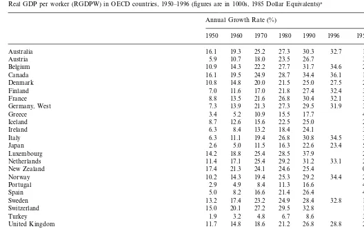
We begin with measures of real GDP (1985 dollar equivalents) per worker (RGDPW). Computations for 1950 – 1990 are based on the variable RGDPW from Penn World Table (PWT) Mark 5.6 (see Summers and Heston, 1991, for a description of the database). Computations for 1995 are based on the variables GDPD (Gross Value Added in US Dollars) and ET (Total Employment) from the OECD ISDB (International Intersectoral) Database for 14 OECD countries. The PWT figures for 1990 are used as benchmarks, and the figures are updated to 1995 on the basis of the growth rate of labor productivity for 1990 – 1995 computed from the ISDB data.
The now familiar convergence story is evident. The coefficient of variation (the ratio of standard deviation to mean) among the 24 OECD countries listed in Table 1 declines by more than half between 1950 and 1990. Results are also shown for a sample of Industrial Market Economies (IMEs), as classified by the World Bank, which consists of all OECD countries except Greece, Portugal, and Turkey. Convergence is even stronger among this group, with the coefficient of variation falling by almost two-thirds. The 14 ISDB countries are by and large the biggest
439
Real GDP per worker (RGDPW) in OECD countries, 1950–1996 (figures are in 1000s, 1985 Dollar Equivalents)a
Annual Growth Rate (%)
1996
1950 1960 1970 1980 1990 1950–90 1950–96
32.7 1.59 1.58
16.1 19.5 24.9 28.7 36.1 1.89 1.79
Canada
21.5 25.0 27.5 2.09 2.07
Denmark 10.8 14.8 20.0
21.8 27.4 32.4 3.41 3.41
Finland 7.0 11.6 17.0
Ireland 6.3 8.4 13.2 18.4
30.8
6.3 11.1 19.4 26.8 34.5 3.97 3.78
Italy
23.4
Japan 2.6 5.0 11.5 16.3 22.6 5.41 4.89
2.46
11.4 17.1 25.4 29.2 33.1 2.52 2.37
Netherlands
25.4
17.4 21.3 24.1 24.6 0.95
New Zealand
Spain 5.0 8.2 16.6 21.4
28.4
13.2 17.4 23.2 24.9 32.8 1.91 2.02
Sweden
Switzerland 15.0 20.1 27.2 29.5 32.8 1.96
3.85 8.6
1.9
Turkey 3.2 4.8 6.7
26.8
11.7 14.8 18.6 21.2 28.8 2.08 2.01
United Kingdom
31.7 36.8 38.8 1.46 1.42
20.5
United States 24.4 30.5
Summary statistics:All24OECD countries
27.3
Mean 9.7 13.5 19.3 23.3
6.3
5.0 5.6 6.2 6.0
440
E
.
N
.
Wolff
/
Structural
Change
and
Economic
Dynamics
11
(2000)
433
–
472
Table 1 (Continued)
Annual Growth Rate (%)
1996 1950–90
1950 1960 1970 1980 1990 1950–96
0.26 0.23
0.32 0.41 0.51 Coeff. of Var.
−0.93 Correlation with 1950 RGDPW
Summary statistics:21Industrial market economies(all countries except Greece,Portugal,and Turkey)
Mean 10.7 14.8 21.0 25.0 29.2
4.0 3.9
Std. Deviation 4.5 4.7 4.6
0.15 0.14
0.32
Coeff. of Var. 0.42 0.22
−0.92 Correlation with 1950 RGDPW
Summary statistics:ISDB-14countries
32.4 29.6
25.5
Mean 10.9 15.1 21.4
Std. Deviation 4.4 4.4 4.3 3.9 3.5 3.7
0.11 0.12
Coeff. of Var. 0.41 0.29 0.20 0.15
Correlation with 1950 RGDPW −0.93
aNote:Sources: own computations from the Penn World Table Mark 5.6 and the OECD ISDB (International Intersectoral) Database. See the text for
441
E.N.Wolff/Structural Change and Economic Dynamics11 (2000) 433 – 472
OECD economies, excluding countries such as Austria, Greece, Iceland, Ireland, New Zealand, Portugal, and Turkey. As a result, the convergence results for the ISDB countries are very similar to those for the 21 IMEs. However, after 1980, the rate of convergence in RGDPW slows markedly in all three samples.
Catch-up is also evident, as indicated by the correlation coefficient between the 1950 RGDPW level and the rate of growth of RGDPW after 1950. The correlation coefficient is −0.93 among all OECD countries, −0.92 among the IMEs, and
−0.93 among the ISDB sample. The results indicate that the countries with the lowest productivity levels in 1950 experienced the fastest increase in labor productivity.
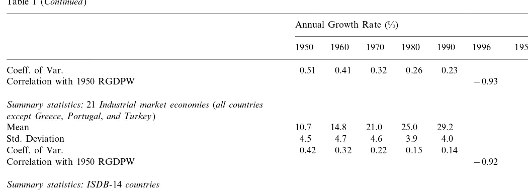
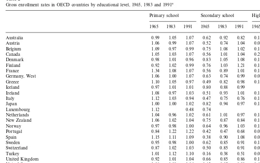
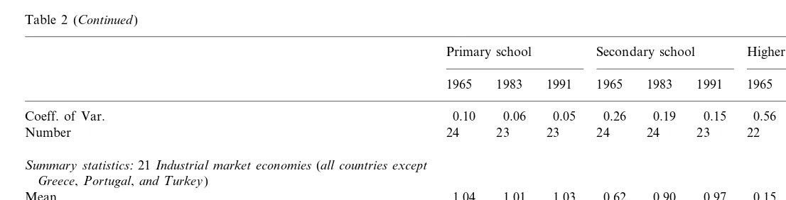
The next five table (Tables 2 – 6) show measures of educational levels among OECD countries. Table 2 shows gross enrollment rates, defined as the ratio of the number of persons enrolled in school to the population of the corresponding age group by educational level. There was almost 100% enrollment at the primary school level and almost no variation among countries in this group. In contrast, the average secondary school enrollment rate increased from 59% in 1950 to 94% in 1991 among all OECD countries and from 62 to 97% among the IMEs. The standard deviation remains fairly constant over time, while the coefficient of variation falls from 0.26 in 1965 to 0.15 in 1991 among all OECD nations and from 0.20 to 0.11 among IMEs — a reflection of the rising mean.
The largest dispersion is found on the higher education level. In 1965, on average, only 13% of college-age adults were enrolled in tertiary school, with the U.S. the highest at 40% and Turkey the lowest at 4% (Spain the lowest at 6% among IMEs). However, by 1991, the average enrollment rate had tripled to 39%, with Canada now leading at 99% and Turkey the lowest at 14% (Ireland the lowest at 24% among IMEs).7 The standard deviation actually rises over time for both
country samples, particularly between 1983 and 1991, while the coefficient of variation falls from 0.56 in 1965 to 0.36 in 1983 and then increases to 0.40 among all OECD countries and falls from 0.51 to 0.27 among the IMEs between 1965 and 1983 and then shoots up to 0.40 in 1991.8
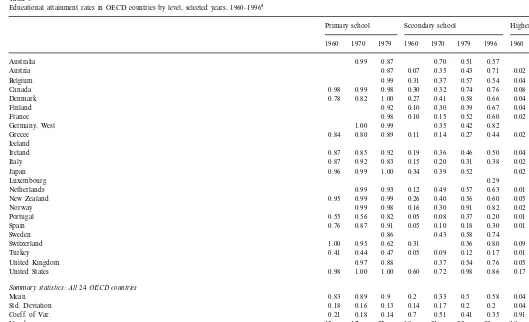
Educational attainment rates, defined as the proportion of the population 25 and over who have attained the indicated level of schooling or greater, are shown in Table 3 for years 1960, 1970, 1979, and 1996. A word should be said about the reliability of the data. Unlike the enrollment rate data of the preceding table, which appear to be relatively consistent over time, there are several anomalies in the attainment rate data. At the primary school level, there appear to be substantial declines in attainment rates for Greece and Ireland between 1960 and 1970; for Australia, Italy, the Netherlands, and the U.K. between 1970 and 1979; and for
7The Canadian figure seems unrealistically high but that is what is reported in the various World Bank data sources.
442
Gross enrollment rates in OECD countries by educational level, 1965, 1983 and 1991a
Primary school Secondary school Higher education
1965 1983 1991 1965 1983 1991
1965 1983 1991
0.82 0.16 0.26 0.39
Australia 0.99 1.05 1.07 0.62 0.92
1.04 0.09 0.25 0.35
0.74 0.52
Austria 1.06 0.99 1.07
1.02 0.15 0.28 0.38
Belgium 1.09 0.97 0.99 0.75 1.08
1.04 0.26 0.42 0.99
1.01
Canada 1.05 1.03 1.07 0.56
1.08 0.14 0.29 0.36
Denmark 0.98 1.01 0.96 0.83 1.05
1.21 0.11 0.31 0.51
1.03
Finland 0.92 1.02 0.99 0.76
1.01 0.18 0.28 0.43
France 1.34 1.08 1.07 0.56 0.89
0.99 0.09 0.30 0.36
0.74
Germany, West 1.06 1.00 1.07 0.63
0.98 0.10 0.17 0.25
Greece 1.10 1.05 0.97 0.49 0.82
0.99 0.29
0.88 0.80
Iceland 0.97 1.01 1.01
1.01 0.12 0.22 0.34
Ireland 1.08 0.97 1.03 0.51 0.93
0.76 0.11 0.26 0.32
0.75
Italy 1.12 1.03 0.94 0.47
Japan 1.00 1.00 1.02 0.82 0.94 0.97 0.13 0.30 0.31
0.74
Luxembourg 1.12 0.48
0.97 0.17 0.31 0.38
Netherlands 1.04 0.96 1.02 0.61 1.01
0.84 0.15 0.28 0.45
0.87
New Zealand 1.06 1.02 1.04 0.75
1.03 0.11 0.28 0.45
Norway 0.97 0.98 1.00 0.64 0.96
0.68 0.05 0.11 0.23
0.47 0.42
Portugal 0.84 1.22 1.22
1.08 0.06 0.24 0.36
Spain 1.15 1.11 1.09 0.38 0.90
0.91 0.13 0.39 0.34
0.85
Sweden 0.95 0.98 1.00 0.62
Switzerland 0.87 1.02 1.03 0.50 0.85 0.91 0.08 0.23 0.29
0.51 0.04 0.07 0.15
0.38
Turkey 1.01 1.12 1.10 0.16
0.85
0.92 1.01 1.04 0.66 0.86 0.12 0.20 0.28
United Kingdom
0.63 0.85 0.90 0.40 0.56 0.76
United States 1.06 1.00 1.04
Summary statistics:all24OECD countries
0.94 0.13 0.27 0.39
0.85 1.03
Mean 1.03 1.03 0.59
0.17
0.10 0.06 0.06 0.15 0.15 0.07 0.10 0.17
443
E
.
N
.
Wolff
/
Structural
Change
and
Economic
Dynamics
11
(2000)
433
–
472
Table 2 (Continued)
Primary school Secondary school Higher education
1965 1983 1991 1965 1983 1991
1965 1983 1991
0.26 0.19 0.15 0.56 0.36 0.40
Coeff. of Var. 0.10 0.06 0.05
23 22 22 23
24 23
Number 24 23 24
Summary statistics:21Industrial market economies(all countries except Greece,Portugal,and Turkey)
0.97 0.15 0.30 0.42
0.62
1.01 1.03 0.90
Mean 1.04
0.10 0.04 0.04 0.10 0.10 0.07 0.08 0.17
Std. Deviation 0.12
0.11
Coeff. of Var. 0.09 0.04 0.04 0.20 0.11 0.51 0.27 0.40
20 19 19 20
21
20 20 21
Number 21
aNote: The gross enrollment rate is defined as the ratio of total enrollment of students of all ages in primary school, and higher education to the
444
Educational attainment rates in OECD countries by level, selected years, 1960–1996a
Primary school Secondary school Higher education
1960 1970 1979 1996 1960 1970 1979 1996
1960 1970 1979
0.70 0.51 0.57 0.22 0.13 0.15
Australia 0.99 0.87
0.43 0.71 0.02 0.03 0.03
0.35 0.06
Austria 0.87 0.07
0.57
Belgium 0.99 0.31 0.37 0.54 0.04 0.03 0.08 0.11
0.74 0.76 0.08 0.10 0.37
0.32 0.17
0.98 0.30
Canada 0.98 0.99
0.41
0.78 0.82 1.00 0.27 0.58 0.66 0.04 0.08 0.11 0.15
Denmark
0.30 0.39 0.67 0.04 0.06 0.11 0.12
0.92 0.10
Finland
0.52 0.60 0.02 0.03 0.14
0.15 0.10
France 0.98 0.10
0.35 0.42 0.82 0.04 0.09 0.13
Germany, West 1.00 0.99
0.27 0.44 0.02 0.04 0.08
0.14 0.12
0.84
Greece 0.80 0.89 0.11
Iceland
0.36
0.87 0.85 0.92 0.19 0.46 0.50 0.04 0.05 0.07 0.11
Ireland
0.31 0.38 0.02 0.03 0.04
0.20 0.08
Italy 0.87 0.92 0.83 0.15
0.39
0.96 0.99 1.00 0.34 0.52 0.02 0.06 0.13
Japan
0.29 0.11
Luxembourg
0.57 0.63 0.01 0.07 0.15
Netherlands 0.99 0.93 0.12 0.49 0.23
0.56 0.60 0.05 0.12 0.27
0.40 0.11
New Zealand 0.95 0.99 0.99 0.26
0.30 0.91 0.82 0.02 0.07 0.11 0.16
0.99 0.98
Norway 0.16
0.37 0.20 0.01 0.02 0.05
0.08 0.08
0.82 0.05
Portugal 0.55 0.56
0.10
0.76 0.87 0.91 0.05 0.18 0.30 0.01 0.04 0.06 0.13
Spain
0.43 0.58 0.74 0.08 0.15 0.13
0.86 Sweden
0.36 0.80 0.09 0.10 0.10
Switzerland 1.00 0.95 0.62 0.31
0.12 0.17 0.01 0.02 0.03 0.06
Turkey 0.41 0.44 0.47 0.05 0.09
0.54 0.76 0.05 0.09 0.12
0.37 0.13
0.88 0.97 United Kingdom
United States 0.98 1.00 1.00 0.60 0.72 0.98 0.86 0.17 0.21 0.30 0.26
Summary statistics:All24OECD countries
0.5 0.58 0.04 0.07 0.12
0.33 0.13
Mean 0.83 0.89 0.9 0.2
0.14 0.17 0.2 0.2 0.04 0.05 0.09 0.05
Std. Deviation 0.18 0.16 0.13
0.41 0.35 0.91 0.78 0.69
0.51 0.37
0.21
Coeff. of Var. 0.18 0.14 0.7
21
12 17 22 18 22 22 19 21 22 22
Number
Summary statistics:21Industrial market economics(all countries except Greece,Portugal,and Turkey)
0.53 0.63 0.05 0.08 0.13
0.37 0.13
Mean 0.81 0.95 0.92 0.21
0.14 0.15 0.19 0.17 0.04 0.05 0.09 0.05
0.28
Std. Deviation 0.06 0.09
0.35 0.26 0.84 0.71 0.65
0.41 0.34
0.69
Coeff. of Var. 0.35 0.06 0.1
19
Number 9 14 19 15 18 19 16 18 19 19
aNote: The educational attainment rate is defined as the proportion of the population 25 and over who have attained the indicated level of schooling or greater. The original data sources are UNESCO,
445
E.N.Wolff/Structural Change and Economic Dynamics11 (2000) 433 – 472
Switzerland over the entire 1960 – 1979 period. Moreover, Australia’s attainment rate at the secondary school level seems to have fallen from 70 to 51% and at the higher education level from 22 to 13% between 1970 and 1979 though both picked up a bit by 1996, whereas Norway’s secondary school rate appears to increase from 30 to 91% from 1970 to 1979 though it then fell back to 82% by 1996. In Canada, the attainment rate at the tertiary level appears to have fallen from 37% in 1979 to only 17% in 1996, despite the huge increase in the enrollment rate at this level, and in New Zealand from 27 to 11% over the same period.
In sofar as enrollment rates have risen in all these countries between 1965 and 1983, it is hard to believe that attainment rates could have fallen. One possible explanation is the immigration of people with low schooling levels to these countries (Australia, perhaps) or the emigration of highly educated individuals (Britain, perhaps). The more likely explanation is errors in the data. These figures are derived from UNESCO Yearbooks and are based on country responses to questionnaires. There may have been changes in country reporting methods over time and/or compilation errors on the part of UNESCO. In any case, I am not in a position to improve on these results.
Despite these reservations, the overall pattern of results is quite sensible. Attain-ment rates, are, not surprisingly, lower than the corresponding enrollAttain-ment rates, since enrollment rates have been increasing over time (that is, attainment rates for the adult population in a given year reflect the enrollment rates when the adults were children). However, changes over time and differences between countries in attainment rates present a similar picture to those based on enrollment rates. Between 1960 and 1996 (1979 in the case of primary schooling), average attainment rates among the adult population rose at all three educational levels. Secondary school attainment rates almost tripled and higher education attainment rates more than tripled. The coefficient of variation in attainment rates falls at all three educational levels, particularly at the higher education level, though the standard deviation increases at both the secondary and tertiary levels.
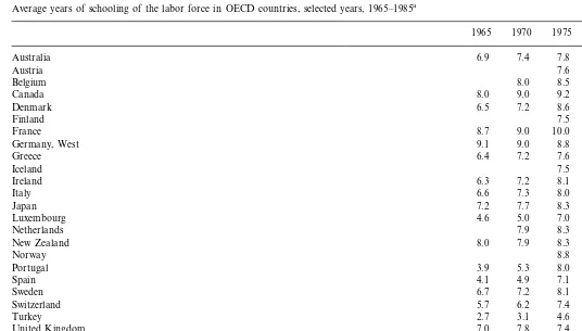
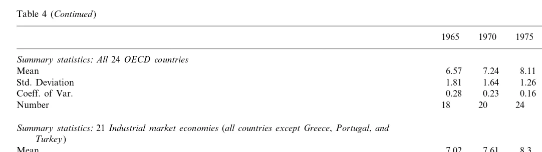
Table 4 shows Kyriacou’s (1991) estimates of mean years of schooling of the labor force from 1965 to 1985. These figures are based on benchmark estimates for mean years of schooling of the labor force for the mid-1970s, which are then updated (or backdated) on the basis of school enrollment rates by level in preceding and succeeding years (see the footnote to Table 4 for details on methodology). There are also some peculiarities in the data here. In both Denmark and France, for example, mean years of schooling seems to have increased between 1965 and 1975 and then declined over the ensuing decade, while in Germany, schooling levels are reported to have fallen slightly from 1965 to 1975.
446
Average years of schooling of the labor force in OECD countries, selected years, 1965–1985a
1985
Belgium 8.0 8.5 8.9 9.4
10.0
United Kingdom 7.0 7.8 7.4
9.8 12.0 12.0 12.1
447
E
.
N
.
Wolff
/
Structural
Change
and
Economic
Dynamics
11
(2000)
433
–
472
Table 4 (Continued)
1985
1965 1970 1975 1980
Summary statistics:All24OECD countries
8.55 8.97
Mean 6.57 7.24 8.11
Std. Deviation 1.81 1.64 1.26 1.19 1.33
0.15
0.28 0.23 0.16 0.14
Coeff. of Var.
23
18 20 24 23
Number
Summary statistics:21Industrial market economies(all countries except Greece,Portugal,and Turkey)
8.8 9.25
7.61
Mean 7.02 8.3
0.99 1.13
Std. Deviation 1.5 1.34 1.09
0.11 0.12
0.18
Coeff. of Var. 0.21 0.13
Number 15 17 21 20 20
aNote: The source is Kyriacou (1991), pp. 61–63. The methodology is as follows: benchmark estimates for mean years of schooling of the labor force were
448 E.N.Wolff/Structural Change and Economic Dynamics11 (2000) 433 – 472
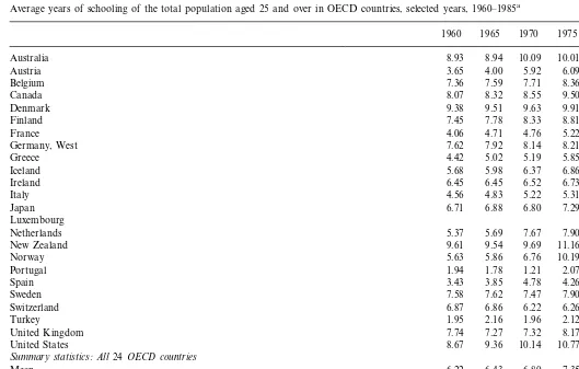
Table 5 shows data for a slightly different concept of mean schooling, that of the total population aged 25 and over, derived from a different source, Barro and Lee (1993). Their method is similar to Kyriacou’s. They begin with benchmark data from UNESCO sources on attainment rates by educational level and then update (or backdate) the attainment figures on the basis of school enrollment rates by level in preceding and succeeding years. Their data show much greater internal consis-tency over time than Kyriacou’s figures. However, their estimates of average schooling for some countries are much lower than the corresponding estimates from Kyriacou (compare Portugal, Spain, and Turkey, in particular). Part of the difference is, of course, that the Barro-Lee figures refer to the total population 25 and over, whereas Kyriacou’s numbers are only for the labor force. However, the discrepancies appear too large to be attributable to this difference alone.
Again, despite the differences in sources and methods, time trends are similar to those shown in Table 4. Average schooling levels rose continuously from 1960 to 1985. The coefficient of variation in schooling levels also shows a decline between 1960 and 1985, though it is much more modest than in the Kyriacou figures. Moreover, the Barro-Lee data show dispersion declining between 1980 and 1985, whereas the Kyriacou data show it rising.
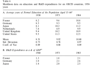
Panel A of Table 6 shows Maddison’s (1987)Maddison’s (1991) estimates of mean years of schooling from 1950 to 1989 for six OECD countries: France, Germany, Japan, the Netherlands, the U.K., and the U.S. These figures also show a sizable increase in educational attainment in the post World War II period, beginning in 1950. On the other hand, the dispersion in schooling levels has remained almost unchanged between 1950 and 1989. However, this result appears to be accounted for by the particular sample of six countries used (the coefficient of variation of mean years of schooling among the same sample of countries on the basis of Kyriacou’s figures is 0.11 in 1970 and 0.11 in 1985).
In summary, two important trends are evident with regard to education. First, there has been a significant increase in average schooling levels in OECD countries since 1950, particularly at the secondary and tertiary levels (primary school levels were already high at the beginning of the post World War II period). Second, the dispersion in educational levels among the various OECD countries has declined substantially over the postwar period, particularly at the secondary level, though it appears to have risen for enrollment rates at the higher education level during the 1980s.
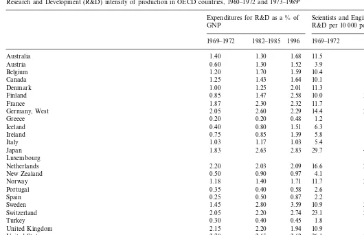
Table 7 shows statistics on two indicators of the technology intensity of produc-tion. The first is the ratio of research and development (R&D) expenditure to GNP,9 and the second is the number of scientists and engineers engaged in R&D
per 10 000 of population. Averages are shown for the 1969 – 1972 and the 1982 – 1985 periods, as well as for 1996. The ranges are considerable. In the 1969 – 1972 period, R&D expenditure as a percent of GNP ranged from lows of 0.20 in Greece and 0.25 in Spain to a high of 2.70 in the U.S. and from a low of 0.20 in Greece
449
Average years of schooling of the total population aged 25 and over in OECD countries, selected years, 1960–1985a
1980
1960 1965 1970 1975 1985
10.24
3.65 4.00 5.92 6.22 6.64
Austria 6.09
9.15
7.36 8.79
Belgium 7.59 7.71 8.36
10.16
8.07 8.32 8.55 9.50 10.37
Canada
9.91 10.14 10.33
9.38
Denmark 9.51 9.63
7.45 7.78 8.33 9.61 9.49
Finland 8.81
6.52
France 4.06 4.71 4.76 5.22 5.97
8.46
7.62 7.92 8.14 8.21 8.54
Germany, West
6.56
4.42 5.02 5.19 5.85 6.73
Greece
Italy 4.56 4.83 5.22 5.31 5.83
8.17
6.71 6.88 6.80 7.29 8.46
Japan
9.61 9.54 9.69 11.16 12.04
New Zealand
10.32
5.63 5.86 6.76 10.19 10.38
Norway
3.43 3.85 4.78 4.26 5.58
Spain
9.45
7.58 9.47
Sweden 7.62 7.47 7.90
9.67
6.87 6.86 6.22 6.26 9.09
Switzerland
Summary statistics:All24OECD countries
7.35 8.08 8.32
6.22
Mean 6.43 6.80
2.42
2.20 2.15 2.26 2.44 2.21
Std. Deviation
0.27
Coeff. of Var. 0.35 0.33 0.33 0.33 0.30
23
23 23 23 23 23
450
E
.
N
.
Wolff
/
Structural
Change
and
Economic
Dynamics
11
(2000)
433
–
472
Table 5 (Continued)
1975 1980 1985
1965
1960 1970
Summary statistics:21Industrial market economies(all countries except Greece,Portugal,and Turkey)
8.87 7.95
7.4 8.67
6.95 6.74 Mean
1.9 1.91 1.7
Std. Deviation 1.81 1.72 1.62
0.19
0.24 0.22
Coeff. of Var. 0.27 0.25 0.22
20
20 20 20 20 20
Number
aNote: The source is: Barro and Lee (1993), Appendix Table A.2. The methodology is as follows: benchmark estimates on attainment rates by six
451
E.N.Wolff/Structural Change and Economic Dynamics11 (2000) 433 – 472
to a high of 2.80 in Sweden in 1982 – 85. In 1996, the ranged went from 0.45 in Turkey to 3.59 in Sweden. The number of scientists and engineers per 10 000 inhabitants ranged from a low of 1.2 in Greece to a high of 29.7 in Japan in the first period, from 2.1 in Turkey to 43.1 in Japan in the second, and from 3.5 in Turkey to 58.2 in Japan in 1996. Two trends are apparent. First, the average R&D intensity increased between the early 1970s and 1996; and, second, the coefficient of variation declined. The trends are stronger among the industrial market economies than among all OECD countries.
These trends appear even stronger in Panel B of Table 6, based mainly on data from Maddison (1987). Among the six countries shown here, mean R&D spending as a percentage of GDP increased from 1.82 in 1960 to 2.52 in 1987, while the coefficient of variation falls from 0.35 to 0.09. Thus, the R&D intensity of production is becoming more similar among this group of OECD countries.
On the surface, at least, there appears to be a direct relation between schooling levels and labor productivity levels, as reported in Table 1. First, the convergence in educational levels among OECD countries appears to correspond to the conver-gence in labor productivity levels over the post World War II period. Second, the
Table 6
Maddison data on education and R&D expenditures for six OECD countries, 1950–1989, selected years
A.A6erage years of Formal Education of the Population Aged15–64a 1973
Japan 8.1 10.2 11.2 11.7
9.9
Std. Deviation 0.73 0.78 0.97 1.17
Coeff. of Var. 0.09 0.08 0.09 0.10
B.R&D Expenditures as a & of GDPb
United Kingdom 2.5 2.4 2.3
United States 2.7 2.4 2.7 2.6
2.38
Mean 1.82 2.05 2.52
Std. Deviation 0.63 0.19 0.25 0.23
Coeff. of Var. 0.35 0.09 0.11 0.09
aSources. 1950–1984: Maddison (1987); 1987: Maddison (1991).
452
Research and Development (R&D) intensity of production in OECD countries, 1960–1972 and 1973–1989a
Scientists and Engineers engaged in Expenditures for R&D as a % of
GNP R&D per 10 000 population
1996
1982–1985 1996 1969–1972
1969–1972 1982–1985
18.6
1.40 1.30 1.68 11.5 31.5
Australia
16.2
0.60 10.1
Austria 1.30 1.52 3.9
7.9
1.20 1.70 1.59 10.4 22.1
Belgium
10.1 14.1 27.0
1.25
Canada 1.43 1.64
15.7
1.00 1.25 2.01 11.3 32.3
Denmark
34.4
Finland 0.85 1.47 2.58 10.0 35.4
18.7
1.87 2.30 2.32 11.7 27.5
France
22.7
2.05 2.60 2.29 14.4 28.7
Germany, West
Ireland 0.75 0.85 1.39 5.8 9.1
10.7
2.20 2.03 2.09 16.6 22.2
Netherlands
Spain 0.25 0.50 0.87 2.2 4.0
24.2
1.45 2.80 3.59 10.9 40.5
Sweden
Switzerland 2.05 2.20 2.74 23.1 21.0 27.7
3.5
0.30 1.8 2.1
Turkey 0.40 0.45
15.5
2.15 2.20 1.94 10.9 24.7
United Kingdom
26.1 30.7 36.4
United States 2.70 2.65 2.62
Summary statistics:All24OECD countries
25.25
Mean 1.20 1.50 1.76 10.49 16.97
10.37
0.72 0.78 0.80 7.44 12.15
453
E
.
N
.
Wolff
/
Structural
Change
and
Economic
Dynamics
11
(2000)
433
–
472
Table 7 (Continued)
Scientists and Engineers engaged in Expenditures for R&D as a % of
R&D per 10 000 population GNP
1996
1982–1985 1996
1969–1972 1969–1972 1982–1985
0.48
Coeff. of Var. 0.60 0.52 0.45 0.71 0.61
Number 23 23 23 23 23 23
Summary statistics:21Industrial market economies(all countries except Greece,Portugal,and Turkey)
27.94 11.79
1.95
1.67 19.13
Mean 1.33
0.67 0.68 0.68 9.37 10.63
Std. Deviation 7.12
Coeff. of Var. 0.50 0.41 0.35 0.60 0.49 0.38
20 20
20 20
20 20
Number
aNote: The original data sources are UNESCO Statistical Yearbook, 1963–1990 and the OECD ANBERD database, 1998 version. Period averages are
454 E.N.Wolff/Structural Change and Economic Dynamics11 (2000) 433 – 472
increase in schooling levels seems to correspond to the growth in labor productivity over this period. Moreover, as productivity and educational levels were growing and converging among OECD countries, so was their R&D intensity of production. We now turn to regression analysis to analyze these relations more systematically.
3. Catch-up models
For heuristic reasons, I begin the econometric analysis with the catch-up model. As noted in the Section 1.2 above, this approach implies that education should be interpreted as a threshold effect and leads to an econometric specification in which the rate of productivity growth is a function of the le6elof schooling. Of course,
one is still left with the difficulty of deciding which year to use for the educational variable. When productivity growth is measured over a short period of time, the model would suggest using educational attainment as of the beginning of the period. However, when productivity growth is measured over a long time period, educational levels will likely be rising and initial education may not be relevant for characterizing the ability of the work force to adopt new technology toward the end of the period. In this case, one might use the average educational level over the period. Of course, as a matter of practicality, one is limited in choice by the available data.
The basic model specification is as follows:
ln(RGDPW1/RGDPW0)/(t1−t0)
=b0+b1 RGDPW0%+b2 INVRATE+b3 RDGNP+b4 EDUC+o (1)
where ln(RGDP1/RGDP0)/(t1−t0) is the annual rate of growth in real GDP (1985
dollar equivalents) per worker from time 0 to1; RGDP0% is RGDP near the beginning of the period; INVRATE is the average investment rate, defined as the ratio of investment to GDP, both in 1985 dollar equivalents, averaged over the period of analysis; RDGNP is the average ratio of R&D expenditures to GNP, averaged over the period; EDUC is a measure of educational input; and o is a stochastic error term.10 Mankiw et al. (1992) provide some theoretical justification
for this approach, deriving this specification from an augmented Solow model. However, one can also be agnostic about the theoretical foundations of the model. The convergence hypothesis predicts that the coefficientb1will be negative (that
is, countries further behind near the beginning of the period will show more rapid increases in GDP per worker). The coefficients of the investment rate (b2), R&D
intensity (b3), and education (b4) should be positive. Results are shown in Table 8
455
Regressions of the annual growth in real GDP per worker (RGDPW) on Initial RGDPW, the investment rate, R&D, and educational enrollment and
attainment levels, all OECD countries, 1950–1990a
AdjustedR2 Standard error
Relative INVRATE R&D Education variable R2 Sample size Education variable
RDGPW55
0.070d 0.82 0.0047 23 PRIM-ENRL
1965
0.336b 0.018b
−0.018d 0.86
(8.77) (2.88) (2.04) (1.90)
0.82
0.074d 0.0048 23 PRIM-ENRL
65–91
0.85 0.81 0.0049 22 UNIV-ENRL1965
−0.017d 0.078c 0.318 0.026
0.032 0.233 0.033c 0.89 0.0043 22 PRIM-ATTN1970
−0.024d
(8.93) (1.28) (1.42) (2.79)
0.83
0.057c 0.0047 22 PRIM-ATTN
1979
0.039 0.264 0.029c 0.88 0.0044 22 PRIM-ATTN60–79
−0.022d
(8.92) (1.60) (1.59) (2.54)
0.80
0.064c 0.0051 22 SCND-ATTN
1970
0.408b −0.009 0.84
−0.017d
(5.62) (2.47) (2.09) (0.78)
0.79
0.064c 0.0052 22 SCND-ATTN
456
Table 8 (Continued)
INVRATE R&D R2 AdjustedR2 Standard error Sample size Education variable
Relative Education variable
RDGPW55
0.83 0.79 0.0052 23 UNIV-ATTN1979
−0.019d 0.065c 0.362b 0.002
0.058c 0.0051 23 MEAN-EDUC
1965
0.072c 0.0050 23 MEAN-EDUC
1980
0.338b 0.004 0.84
−0.018d
(7.97) (2.68) (1.92) (0.96)
0.80
0.072c 0.0050 23 MEAN-EDUC
1985
0.065b 0.0051 23 MEAN-EDUC
65–85
0.312 0.000 0.83
−0.018d
(7.57) (2.07) (1.72) (0.05)
0.068c 0.82 0.0048 23 BL-EDUC
1960
0.069c 0.0049 23 BL-EDUC
1965
0.349b −0.001 0.84
−0.016d
(5.34) (2.72) (2.02) (1.36)
0.83 0.80 0.0050 23 BL-EDUC1970
−0.016d 0.068c 0.326b −0.001
(5.08) (2.59) (1.84) (0.79)
0.84 0.81 0.0049 23 BL-EDUC1975
−0.015d 0.072c 0.325b −0.001
(2.77) (1.88)
(4.86) (1.24)
0.82
0.078d 0.0047 23 BL-EDUC
1980
0.358c −0.001b 0.85
−0.014d
(4.13) (3.09) (2.15) (1.84)
0.85 0.81 0.0048 23 BL-EDUC1985
−0.014d 0.075d 0.343b −0.001
(4.17) (2.93) (2.03) (1.57)
0.81
0.072c 0.0048 23 BL-EDUC
60–85
0.055b 0.0053 24 SCND-ENRL
65–91
0.013 0.000 0.81
−0.017d
457
Table 8 (Continued)
Education variable R2 AdjustedR2 Standard error Sample size Education variable
Relative INVRATE R&D
RDGPW55
0.84 0.80 0.0051 22 UNIV-ENRL65–91
0.071c
−0.020d 0.005 0.037
(7.36) (2.38) (0.29) (1.65)
0.86 0.83 0.0046 22 PRIM-ATTN60–79
0.031
−0.022d 0.009 0.031c
(1.18) (0.70)
(8.38) (2.52)
0.78
0.041 0.028 −0.012 0.82 0.0054 22 SCND-ATTN60–79
−0.016d
(4.76) (1.28) (1.47) (0.78)
0.83 0.78 0.0053 22 UNIV-ATTN60–79
0.035
−0.015d 0.026 −0.039
(4.87) (1.07) (1.61) (1.07)
0.77
0.060b 0.0052 23 MEAN-EDUC
65–85
aNote: The absolute value of t-ratios are shown in parentheses below the coefficient estimate.See footnotes to Tables 2 and 3 Tables 4–7 for sources and
methods. Key:Dependent variable: ln(RGDPW90/RGDPW50)/40.RGDPWt: GDP per worker in yeart, measured in 1985 international prices (in units of
$10 000).Source: Penn World Table Mark 5.6.Relative RGDPW55:RGDPW level of the country relative to the RGDPW level of the U.S. in 1955.Source:
Penn World Table Mark 5.6.INVRATE: Ratio of investment to GDP (both in 1985 dollar equivalents) averaged over the regression period.Source: Penn World Table Mark 5.6.RDGNP: Expenditure for R&D as a percentage of GNP. Source: UNESCO Statistical Yearbook,1963–1990.SCIENG: Scientists and
engineers engaged in R&D per 10 000 of Population. Source: UNESCO StatisticalYearbook, 1963–1990.PRIM-ENRLt: Total enrollment of students of all
ages in primary school in yeartas aproportion of the total population of the pertinent age group. PRIM-ENRLt−t’:Average primary school enrollment rate
intandt%.SCND-ENRLt:Total enrollment of students of all ages in secondary school in year t as aproportion of the total population of the pertinent age
group. SCND-ENRLt-t’:Average secondary school enrollment rate intandt%.UNIV-ENRLt: Total enrollment of students of all ages in higher education
in year t as aproportion of the total population of the pertinent age group. UNIV-ENRLt-t’:Average tertiary school enrollment rate intandt%.PRIM-ATTNt:
Proportion of the population age 25 and over who have attended primary schoolor higher in yeart.SCND-ATTNt: Proportion of the population age 25
and over who have attended secondary schoolor higher in yeart.UNIV-ATTNt: Proportion of the population age 25 and over who have attended an
institution ofhigher education in yeart.MEAN-EDUCt: Mean years of schooling of the labor force in year t, from Kyriacou (1991).MEAN-EDUCt−t’:
Average years of schooling fromttot%.BL-EDUCt: Mean years of schooling of the of the total population aged 25 and over in yeart,from Barro and Lee
(1993). BL-EDUCt-t’: Average years of schooling fromttot%.
bsignificant at the 10% level, two-tail test.
csignificant at the 5% level, two-tail test.
458 E.N.Wolff/Structural Change and Economic Dynamics11 (2000) 433 – 472
for all OECD countries over the 1950 – 1990 period and for a variety of educational measures.11
The RGDPW level of the country relative to the U.S. level is by far the most powerful explanatory variable in accounting for differences in labor productivity growth among OECD countries. By itself, the catch-up variable explains 74% of the variation in RGDPW growth over the 1950 – 1988 period. The coefficient of INVRATE is positive and significant at the 5% level or greater except in three cases where it is significant at the ten percent level. The average investment rate, together with the catch-up variable, explains 80% of the variation in RGDPW growth. R&D intensity is significant at the 10% in almost all cases.
The educational enrollment rates have positive coefficients in all but one case and of these are significant in only one case — the primary enrollment rate in 1965, which is significant at the 10% level. This is the most unlikely case, since primary education enrollment rates show little variation among OECD countries.
The attainment rates by level of schooling have positive coefficients in only half the cases. While the coefficients are insignificant for secondary and university attainment, they are significant for primary school attainment levels (at the 5% level for 1970 and the average rate over the 1960 – 79 period and at the 10% level for 1979). The results for primary education are unexpected, because this is the level of schooling that would appear to have least relevance to the types of sophisticated technology in use among OECD countries in the post World War II period. Also there is little variation in this measure among OECD countries, except for Greece, Portugal, and Turkey (the three non-industrial market economies). However, even when these three countries are excluded from the sample, the coefficient remains significant at the 5% level. I shall comment more on this result in the conclusion. Because of the anomalies in this data series discussed above, I have also used the average value of the attainment rates over the four periods, 1960, 1970, 1979, and 1996. When there are missing values, I use the average of the data points that are available. This method has the added advantage of eliminating most of the missing observations for 1970. However, the results are virtually unchanged. The coefficient of the average primary attainment rate is significant at the 5% level, while that of the secondary and tertiary attainment rates remain insignificant.
The next two panels show results for mean educational levels. The first of these is based on the Kyriacou data on average schooling for the labor force. The coefficients of these educational variables are positive in only four of six cases and not significant in any. The second panel uses the Barro-Lee data on average education for the adult population. The coefficients of these variables are all insignificant and, indeed, all have negative values.
At first glance, the disparity in results for these two measures of mean schooling is, to say the least, disquieting. However, it should be noted that the schooling of the labor force should, in principle, have more relevance to the growth in labor productivity than the educational attainment of the total adult population, and the regression results confirm this. Still, one would have expected a fairly high
459
E.N.Wolff/Structural Change and Economic Dynamics11 (2000) 433 – 472
correlation between these two indices of educational achievement. Instead, the correlation coefficients are rather low (for example, 0.54 between MEAN-EDUC75
and BL-EDUC75). It appears more likely that differences in sources and methods
used to construct the two series are responsible for the discrepancy in econometric results.
The results are quite similar when SCIENG, the number of scientists and engineers engaged in R&D per 10 000 population, is substituted for RDGNP, as shown in Panel B of Table 8. The coefficients of the variable SCIENG are generally somewhat less statistically significant than RDGNP, as are the coefficients of INVRATE. However, the coefficients of the education variables are essentially unchanged.12
An anonymous referee suggested that the use of cross-sectional regressions, where variables are averaged over time, might cause relatively low variability of the education variables and thus result in low significance levels. In Table 9I use pooled cross-section, time-series data for the 24 OECD countries and periods 1960 – 1973 and 1973 – 1990. Due to data limitations, the only education variables that could be used are the enrollment rates. The regression results are similar to those in the cross-section analysis of Table 8. The coefficients of the enrollment rates remain insignificant. In fact, for the secondary and tertiary levels, the coefficients are negative. The catch-up term is less significant than before (because of the shorter time period), as are the R2 and adjusted R2 statistics, but the investment rate
variable is stronger. There is little change in the R&D variables.
4. Human capital models
I next turn to the human capital model, which posits a positive relation between the rate of productivity growth and therate of changeof schooling levels. For this, I use the same specification as Eq. (1), except that I substitute the change in educational level for the educational level itself. The model becomes:
ln(RGDPW1/RGDPW0)/(t1−t0)
=b0+b1 RGDPW0%+b2 INVRATE+b3 RDGNP+b4D(EDUC)+o (2)
whereD(EDUC) is the change in level of schooling. Results are shown in Table 10 for all OECD countries over the 1960 – 1990 period. I have used this shorter period (instead of 1950 – 1990), since data on schooling levels are not available for the 1950s for the full set of OECD countries.
The results are again disappointing. Of the 12 forms used, the coefficient of the change in schooling is positive in all cases but statistically significant in only two: the change in university enrollment rates at the 10% level and the change in
460
Pooled cross-section, time-series regressions of the annual growth in real GDP per worker (RGDPW) on initial RGDPW, the investment rate, R&D, and
educational enrollment levels, all OECD countries, 1960–1973 and 1973–1990a
R2 AdjustedR2 Standard error Sample size Education variable
R&D
Relative RDGPW55 INVRATE Education variable
(A)R&D6ariable:RDGNP
0.45 0.41 0.0145 46
−0.032d 0.145d 0.691b
(4.77) (3.01) (1.72)
0.46 0.41 0.0146 46 PRIM-ENRL
−0.032d 0.149d 0.723b 0.021
(3.06) (1.78)
(4.69) (0.80)
0.52
0.157d 0.591 −0.013 0.56 0.0132 46 SCND-ENRL
−0.021d
(B)R&D 6ariable:SCIENG
0.43 0.38 0.0150 46 PRIM-ENRL
0.029
aNote: The sample consists of pooled cross-section, time-series data for periods 1960–1973 and 1973–1990. The absolute value oft-ratios are shown in
parentheses below the coefficient estimate. See Table 8 for definitions of the variables.
b significant at the 10% level, two-tail test.
c significant at the 5% level, two-tail test.
461
Regressions of the growth in GDP per worker (RGDPW) on initial RGDPW, the investment rate, R&D intensity, and the change in educational
enrollment and attainment levels, all OECD countries, 1960–1990a
Standard error Sample size
Relative RDGPW65 INVRATE R&D Education variable R2 AdjustedR2 Education variable
(A)R&D6ariable:RDGNP
0.0048 23
0.0047 22 DUNIV-ENRL91–65
0.83
−0.022d 0.058c 0.467c 0.489b 0.86
(2.36) (2.57) (1.87)
(8.10)
0.74
0.050 0.187 0.127 0.80 0.0052 21 DSCND-ATTN96–60
−0.017d
(B)R&D 6ariable:SCIENG
0.0048 23
0.045c DSCND-ENRL
91–65
−0.017d 0.031b 0.454c 0.85 0.82
(8.69) (2.11) (2.14) (2.09)
0.0052 22 DUNIV-ENRL91–65
0.79 0.83
−0.019d 0.044 0.022 0.353
(1.49)
(7.30) (1.54) (1.26)
0.0052 21 DSCND-ATTN96–60
0.74
0.83 0.79 0.0051 23 DBL-EDUC85–60
0.018
−0.017d 0.049b 0.015
(1.22)
(1.78) (0.45)
(7.60)
aNote: The dependent variable is ln(RGDPW
90/RGDPW60)/30. The absolute value oft-ratios are shown in parantheses below the coefficient estimate.
See Table 8 for definitions of the variables. In addition, a ‘D’ indicates the annual change in the variable over the period.
bsignificant at the 10% level, two-tail test.
csignificant at the 5% level, two-tail test.
462 E.N.Wolff/Structural Change and Economic Dynamics11 (2000) 433 – 472
secondary school attainment rates at the 5% level (with SCIENG as the R&D variable). One possibility, at least for the educational attainment rate and the Kyriacou mean schooling level data, is that the anomalies in the basic data are undermining the regression results (the enrollment rate data seem sensible, as do the Barro-Lee mean schooling levels). I eliminated all observations that seemed to be unreasonable and reran the regressions. The results were virtually unchanged.
Another possibility is that there is both a threshold effect, as well as a positive influence of the growth in human capital on labor productivity growth. The same 6 equations were re-estimated with initial level of schooling also included (results not shown). In all twelve cases, the change in schooling remains insignificant (including the case of the university enrollment rate).
A second dataset covering the period from 1950 to 1989 for six OECD countries (France, Germany, Japan, the Netherlands, the U.K. and the U.S.) was also used, derived mainly from data provided in Maddison (1987) Maddison (1991) Maddison (1993a,b). These sources provide figures on actual capital stocks, as opposed to investment rates. As a result, following Mankiw et al. (1992), it is possible to use a Cobb-Douglas production function, augmented with human capital, as follows:
LPRGRTHt
where LPRGRTHth is country h’s annual rate of labor productivity growth, RELTFPthis countryh’s total factor productivity (TFP) relative to the U.S. level at the start of each period, KLGRTHthis countryh’s rate of capital-labor growth, and EDUCGRTHthis the annual rate of growth in mean education in countryh, ande¨ is a stochastic error term.13
The regression analysis is conducted as a pooled cross-section covering six countries and four time period — 1950 – 1960, 1960 – 1973, 1973 – 79 and 1979 – 1989.
As with the Penn World Table Mark 5.6 data, the results (see Table 11) generally show no statistically significant effect of the growth in mean education on the growth in labor productivity. Indeed, the coefficient of educational growth is negative in the first two specifications. When a term for initial education is included (the third specification), the coefficient on educational growth turns positive but remains insignificant. However, one surprise is that the coefficient on initial education (EDUC0) isnegati6eand significant at the one percent level. Even when
the variable for the growth in mean education is dropped, the coefficient on initial education remains negative and significant at the one percent level (result not shown). One possible reason is that the variable for initial education picks up part of the catch-up effect (note that the coefficient and significance level of RELTFP both fall when EDUC0 is included in the equation). In other words, a low initial
schooling level is directly associated with a low initial TFP level.
I next included a6intage effect in Eq. (3). This is measured by AGEKCHGth , the annualized change in the average age of countryh’s capital stock over periodt(see
13TFP is defined as ln TFP
t
h, whereYhis the total output of country
463
Regressions of annual labor productivity growth (LPGRTH) on the relative TFP level, capital-labor growth, R&D intensity, and the growth in mean
education, six OECD countries, 1950–1989a
R2 AdjustedR2
RELTFP KLGRTH EDUCGRTH EDUC0 AGEKCHNG RDGDP Standard error Sample size
0.68 0.65 0.011 24
aNote:t-ratios are shown in parentheses below the coefficient estimate. Observations are for France, Germany, Japan, the Netherlands, the U.K. and the
U.S. for four time periods: 1950–1960, 1960–1973, 1973–1979, and 1979–1989. The data source is Maddison (1991), unless otherwise indicated. Key:RELTFP: percentage difference of country’s TFP from U.S. TFP at the beginning of the period.KLGRTH: country’s annual rate of capital-labor growth.EDUCGRTH: country’s annual rate of growth in mean education. Sources. 1950 and 1973: Maddison (1987). 1989: Maddison (1991). 1960
interpolated from data from Christensen et al. (1980). 1979: interpolated from data in Maddison (1987).EDUC0:country’s level of mean education at the
beginning of the period.AGEKCHNG: annualized change in the average age of country’s capital stock over the period.RDGDP: Ratio of R&D expenditures to GDP, averaged over the period. The data are not available before 1960. Sources. 1960–1983: Maddison (1987); 1984–89: UNESCO Statistical Yearbook, various years.
bsignificant at the 10% level.
csignificant at the 5% level.
464 E.N.Wolff/Structural Change and Economic Dynamics11 (2000) 433 – 472
Wolff, 1994, for more details). The results (specification 5) do show a very strong vintage effect (the coefficient of AGEKCHG is negative and significant at the one percent level). Moreover, the coefficient of the growth in mean education is positive and now significant at the 10% level. Moreover, when initial education is included, its coefficient, while still negative, is no longer statistically significant (results not shown). In the final specification, I included R&D intensity, though this variable is available only for 1960 and later. In this case, the coefficient of the growth in mean education becomes insignificant.14
5. Interactions with technical change
There is now a voluminous literature supporting the argument that the rate of productivity growth of a country is strongly related to the R&D intensity of its production (see, for example, Griliches, 1979, a review of the literature). Moreover, the Arrow and Nelson-Phelps models suggest that there may be interaction effects between the educational level of the work force and the R&D intensity of a country. I introduce the interaction effect into the model as follows:
ln(RGDPW1/RGDPW0)/(t1−t0)
=b0+b1 RGDPW0%+b2 INVRATE+b3 EDUC+b4 RDGNP
+b5 RD*EDUC+o (4)
I use two measures for R&D intensity. The first is the average ratio of R&D expenditure to GNP over the period (RDGNP), and the second is the average number of scientists and engineers engaged in R&D per 10 000 of population over the period (SCIENG). For the first measure, the coefficientb4is usually interpreted
as the rate of return to R&D.
An interaction term is included between EDUC and R&D, because, according to the Arrow and Nelson-Phelps models, a more educated labor force should be more successful in implementing the fruits of the R&D activity. For example, it is frequently argued that the Japanese economy is successful in adapting new technol-ogy to direct production because of the high level of education of its workforce. In this sense, of two countries with the same R&D intensity but different education levels, the one with the more educated labor force should adopt new technology more quickly and effectively and this should show up in higher measured productiv-ity growth.15This formulation is admittedly crude and specification problems might
arise if, for example, the variability in the education variable is low enough to cancel out the variability in the R&D variable. In this case, the interaction term might also show low explanatory power.
Results for all OECD countries over the 1960 – 1990 period are shown in Table 12 (note that these results differ somewhat from those of Table 8, whose regressions
14This set of results remains virtually unchanged even when country dummy variables are included in the various regression equations (results not shown).
465
Regressions of the annual growth of real GDP per worker (RGDPW) on initial RGDPW, the investment rate, R&D intensity, schooling, and the
interaction between schooling and R&D, all OECD countries, 1960–1990a1
R&D EDUC*R&D R2 AdjustedR2 Standard error Samp size Education
INVRATE Education
0.66 0.006 23 SCND-ENRL65–91
−0.023d 0.092c 0.007 0.58c 0.72
(5.02) (2.69) (0.61) (2.41)
0.64 0.006 23 SCND-ENRL65–91
−0.021d 0.098c −0.002 0.02 0.008 0.72
(3.61) (2.61) (0.09) (0.02) (0.44)
0.68 0.006 22 UNIV-ENRL65–91
−0.026d 0.116d 0.035 0.55 0.74
(5.53) (3.51) (1.43) (2.18)
0.67 0.006 22 UNIV-ENRL65–91
−0.027d 0.111d 0.056 0.74 −0.009 0.75
(0.33)
(4.30) (3.03) (0.82) (1.15)
0.66 0.007 21 SCND-ATTN1970
−0.018d 0.103d −0.012 0.67c 0.73
(3.83) (3.05) (1.02) (2.51)
0.022 0.77 0.70 0.006 21 SCND-ATTN1970
−0.047b
−0.015d 0.135d −0.09
(1.58)
(2.97) (3.71) (2.08) (0.19)
0.66 0.006 21 UNIV-ATTN1970
−0.019d 0.097c −0.032 0.59c 0.73
(3.86) (2.77) (0.91) (2.24)
0.72 0.006 21 UNIV-ATTN1970
−0.015d 0.129d −0.169c −0.02 0.081 0.79
(1.43)
(3.30) (3.68) (2.36) (0.05)
0.67 0.006 23 MEAN-EDUC1975
−0.023d 0.105d 0.001 0.52c 0.73
(5.91) (3.34) (1.11) (2.16)
0.001 0.73 0.66 0.006 23 MEAN-EDUC1975
0.001
−0.023d 0.110d 0.11
(5.31) (3.13) (0.22) (0.09) (0.35)
0.66 0.006 23 BL-EDUC1970
−0.019d 0.100d −0.001 0.55c 0.72
(3.45) (3.15) (0.57) (2.29)
0.001 0.72 0.64 0.006 23 BL-EDUC1970
−0.001
−0.018d 0.108d 0.20
(2.87) (0.67) (0.22) (0.43)
(3.01)
aNote: The absolute value of t-ratios are shown in parentheses below the coefficient estimate. A constant term is included in the equation but its coefficient
is not shown. The dependent variable is ln(RGDPW90/RGDPW60)/30.
bsignificant at the 10% level, two-tail test.
csignificant at the 5% level, two-tail test.