Decadal climate variability PIB08

(1)

IN BRIEF

A number of studies indicate an apparent slowdown in the overall rise in global average surface temperature between roughly 1998 and 2014. Most models did not predict such a slowdown—a fact that stimulated a lot of new research on variability of Earth’s climate system. At a September 2015 workshop, leading scientists gathered to discuss current understanding of climate variability on decadal timescales (10 to 30 years) and whether and how prediction of it might be improved.

Proceedings of a Workshop

FRONTIERS IN DECADAL

CLIMATE VARIABILITY

Proceedings of a Workshop

July 2016

Frontiers in Decadal Climate Variability

There is broad agreement in the scientiic community that Earth is warming steadily through time. Since 1880, the average temperature at Earth’s surface has increased by about 0.85°C. Most of this increase (about 0.72°C) has occurred since 1951. In the 2000s, however, the rise in surface temperature slowed down, stimulating many ques-tions. Given that human inluence on the climate did not slow down during this period, where did the heat go? Are measurements inaccurate?

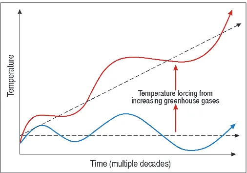
Many researchers focused their attention on the climate system itself, which is known to vary across seasons, decades, and other timescales. Several natural variables produce “ups and downs” in the climate system, which are superimposed on the long-term warming trend due to human inluence (see Figure 1).

Understanding decadal climate variability is impor-tant not only for assessing global climate change but also for improving decision making related to infrastructure, water resources, agriculture, energy, and other realms. Like the well-studied El Niño and La Niña interannual varia-tions, decadal climate variability is associated with speciic regional patterns of temperature and precipitation, such as heat waves, cold spells, and droughts.

WHAT FACTORS CONTRIBUTE TO CLIMATE

VARIABILITY?

Natural climate variability arises from two different sources: (1) internal variability from interactions among compo-nents of the climate system, for example, heat transfer between the ocean and the atmosphere or within varying depths of the ocean, and (2) natural external forcings that

can push Earth toward warming or cooling, for example, volcanic eruptions and solar variations. Changes in human-caused factors,

such as the emission of greenhouse gases (GHGs) and aerosols, also exert external forcing on the climate system. The climate we experience is the combination of all of these factors.

A major theme of discussion at the workshop was the extent to which natural variability modulated human-caused climate change during the recent warming

(2)

slowdown, as well as during past periods of more rapid warming, such as from 1970 to 1998. A second theme was the extent to which external forcing played a role. A third theme focused on the possibility that global mean surface temperature (GMST) rise did not slow down, but rather that biases in tempera-ture data made it appear as though it did. Workshop participants also pointed to the need to reduce miscommunication by being more consistent in the way climate trends are determined and presented.

INTERNAL VARIABILITY IN

THE CLIMATE SYSTEM

As much as 93 percent of the heat trapped by greenhouse gases (GHGs) is stored in the ocean. In comparison, the lower atmo-sphere and sea surface—where global surface temperature is measured—are very small heat reservoirs. Thus, many participants stressed the importance of understanding how and

why heat moves within the climate system to determine how it would affect surface temperature and other measures of climate change.

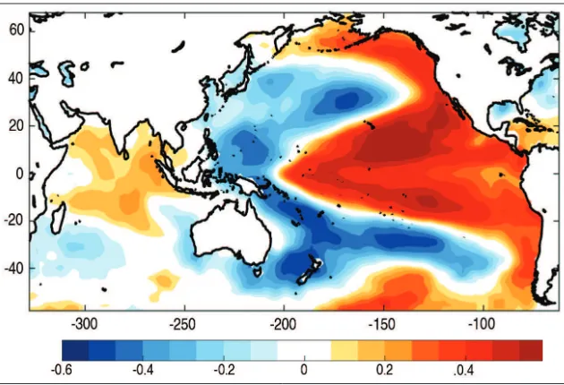
A number of participants noted that Paciic Decadal Variability (PDV) is a major driver of global climate vari-ability (see Figure 2). During the positive (or “warm”) phase of the PDV, the eastern Paciic Ocean becomes warmer and part of the western Paciic Ocean cools; during the negative (or “cool”) phase, the opposite pattern occurs. Two indices are used to track the PDV: the Paciic Decadal Oscillation, or PDO, and the Interdecadal Paciic Oscillation, or IPO.

Several participants presented evidence linking the phases of the IPO to decadal variability in GMST. The recent slowdown in GMST occurred when the IPO was in

Is Global Mean Surface Temperature the right metric of climate change?

One of the ongoing challenges in meas-uring climate change is the question of where to take Earth’s temperature. Several participants said that global mean (average) surface temperature (GMST) is not an adequate metric, in large part because the ocean is capable of storing large amounts of heat below the surface. Some participants suggested that, because water expands as it is heated, global average sea-level together with GMST would be a better metric of climate change.

Figure 2. Some participants said that Paciic Decadal Variability (PDV) is a major driver of global climate variability. During the warm phase of the PDV, shown in this igure, sea surface temperatures in the eastern Paciic are warm, while the northwest and southwest Paciic are cool. During the negative phase of the PDV, the pattern is reversed.

its negative phase (2000–2013), whereas the IPO was in its positive phase during a previous period of faster warming (late 1970s to late 1990s; see Figure 3). There is also evidence of the inluence of the IPO in other slowdown periods in the past (e.g., mid-1940s to late 1970s).

Swings in North Atlantic sea surface temperatures are the central feature of Atlantic Multidecadal Variability (AMV), which has been shown to have signiicant regional and global climate impacts. The mechanisms associated with the AMV are not as well understood as those of PDV, although some studies suggest that it may be driven by changes in the Atlantic Meridional Overturning Circulation (AMOC), which is a major feature of ocean circulation in the Atlantic.

(3)

Regional climate patterns can be inluenced simul-taneously by Atlantic and Paciic variability. For example, although the recent U.S. drought is clearly related to the negative phase of the IPO, one participant presented evidence that the effects of the AMV may be more signiicant than is commonly assumed. The extremely dry conditions of the Dust Bowl and the persistent Texas drought in the 1930s and the 1950s corresponded with warm phases of the AMV. Droughts were less severe during the cold phases of the AMV.

A number of studies have suggested that storage of heat in the deeper ocean may explain the slowdown in surface temperature trend. Evidence was presented that the top 100 m layer of the Paciic Ocean was cooler during the slowdown because heat was transported into the Indian Ocean and deeper into the Paciic. Indian Ocean heat content increased abruptly, which could account for greater than 70 percent of the global ocean heat gain in the upper 700 m during the past decade.

CHANGES IN EXTERNAL FORCINGS

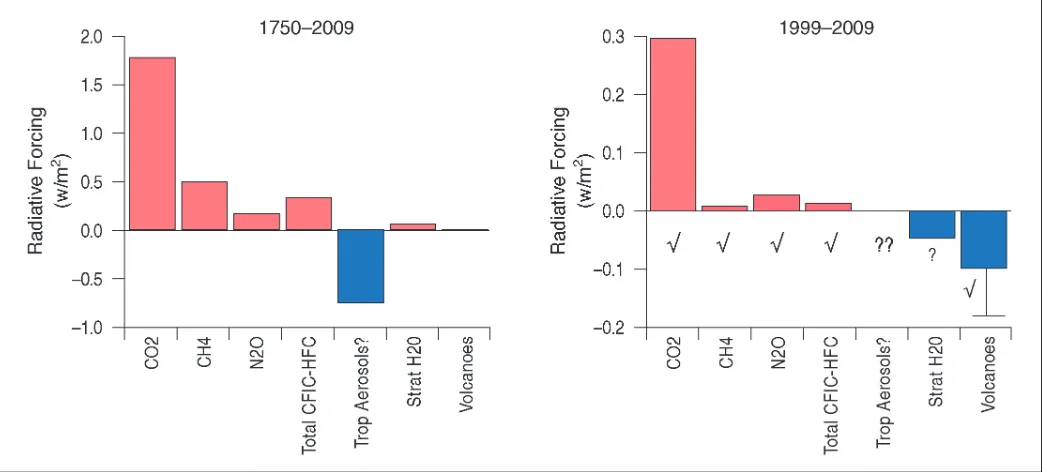
Evidence was presented to show that natural external forcings also played a role in the GMST slowdown. To isolate how external forcings changed during the slowdown period, one participant compared warming and cooling effects of various external forcings from 1750–2009 (Figure 4, left) to 1999–2009 (Figure 4, right).

These data show volcanic eruptions may have contrib-uted signiicantly to recent variability, and that their contributions have been underrepresented in models due to

the lack of availability of the more recent observed volcanic aerosol forcing data. Satellite data that were not available prior to the early 2000s show the inluence of a series of eruptions after 2005. For example, the Nabro volcanic eruption in 2011 cooled tropical sea surface temperatures by a few tenths of a degree.

Data also indicate a decrease in stratospheric water vapor, which is a natural greenhouse gas. Limited data before the mid-1990s suggest that stratospheric water vapor increased up to the year 2000, possibly contributing to the accelerated warming from 1980 to 2000. Water vapor dropped signiicantly after 2000 and stayed low through much of the 2000s.

EXAMINING CLIMATE TRENDS

Calculating climate trends requires selecting a baseline period against which any trend is compared. Challenges arise when baseline periods differ or are not clearly deined. A paper released in Science by Karl et al. (2015) comparing the recent trend to the baseline 1951 to 2012, suggested that the slowdown during the early 2000s did not occur but was rather partly the result of biases and gaps in temper-ature data. Recent efforts by the National Oceanic and Atmospheric Administration (NOAA) to improve datasets were presented at the workshop. However, other partici-pants said that the selection of the baseline 1951 to 2012 did not provide a useful comparison for the recent trend, because it combines a period of slower warming (~1951– 1976) and a period of more rapid warming (~1977–1998).

(4)

OVERCOMING DATA LIMITATIONS

The ability to improve understanding of decadal climate variability is limited by the relatively short length of many climate records. Limited spatial coverage of observations also presents a challenge. Several participants discussed their work illing in observational records.

For example, while it is known that rapid warming occurred from 1910–1939 despite weak external forcing, there are very few records that might provide insight as to why that occurred. However, information about past climate conditions can be found in historical records and “proxy” indicators, such as polar ice caps, tree rings, and corals. For example, one participant presented a study of manganese in coral records, which provides important information about wind direction and El Niño phases in the past.

TOWARD IMPROVED PREDICTION OF

DECADAL VARIABILITY

The degree to which climate is predictable on decadal timescales has enormous societal relevance. For example,

what if decision makers knew they had 30 years versus 10 years to prepare for the large shifts in drought frequency and intensity expected in western North America?

Several participants shared research that assesses decadal predictive capability of current models. Although much progress has been made, decadal climate prediction is still in the early stages of development. For example, the Interdecadal Paciic Oscillation (IPO) phase might explain much of the slowdown in GMST rise, but it is not yet fully understood what triggers changes in IPO phases. A deeper understanding of causal mechanisms will be necessary to predict how and when slowdown-like features will occur, and how these features will manifest regionally.

Several participants said that the slowdown has likely ended as of 2015. Predictions of GMST in the next decades will require a better understanding of many factors, for example, how and where heat is stored in the Paciic, Atlantic, and Indian Oceans.

DISCLAIMER: This Proceedings of a Workshop—in Brief was prepared by Amanda Purcell and Nancy Huddleston as a factual summary of what occurred at the workshop. The planning committee’s role was limited to planning the workshop. The statements made are those of the authors or individual meeting participants and do not necessarily represent the views of all meeting participants, the planning committee, or the National Academies of Sciences, Engineering, and Medicine.

PLANNING COMMITTEE ON FRONTIERS IN DECADAL CLIMATE VARIABILITY: A WORKSHOP—Gerald A. Meehl (Chair), National Center for Atmospheric Research, Boulder, CO; Kevin Arrigo, Stanford University, CA; Shuyi S. Chen, University of Miami, FL; Lisa Goddard, Columbia University, Palisades, NY; Robert Hallberg, Princeton University and National Oceanic and Atmospheric Administration, Princeton, NJ; David Halpern, National Aeronautics and Space Administration Jet Propulsion Laboratory, Pasadena, CA.

SPONSORS: This workshop was supported by the U.S. Department of Energy, the National Aeronautics and Space Administration, the National Oceanic and Atmospheric Administration, and the National Science Foundation.

Division on Earth & Life Studies

For more information, contact the Board on Atmospheric Sciences and Climate at (202) 334-3512 or visit http:/national

academies.org/basc. Frontiers in Decadal Climate Variability—Proceedings of a Workshop can be purchased or downloaded