CONTAGIOUS EFFECTS OF OIL PRICES ON ASIAN
STOCK MARKETS’ BEHAVIOUR
Jok-Tong Wan
Faculty of Economics and Business, Universiti Malaysia Sarawak (UNIMAS) ([email protected])
Evan Lau
Faculty of Economics and Business, Universiti Malaysia Sarawak (UNIMAS) ([email protected])
Rayenda Khresna Brahmana
Faculty of Economics and Business, Universiti Malaysia Sarawak (UNIMAS) ([email protected])
ABSTRACT
The main objective of this study is to examine the stock markets’ shock due to the effect of the price of oil in the East Asia Region. Particularly, this study examines if there is stock market interdependence during global oil price shocks (sudden changes) for a sample of five total oil importers (the Philippines, Hong Kong SAR, Taiwan, South Korea, and Japan), four net oil importers (Indonesia, Singapore, Thailand, and China), and one net oil exporter (Malaysia) between 1999 and 2014. From the result, an oil price change is collectively found to have a small but significant positive impact on the stock markets, in particular where a sudden decrease in oil prices tends to cause a stock market downturn and volatility. The world economy’s spending, financial investments in oil futures and foreign investment by oil rich nations are some underlying motives for inducing this oil-stock positive relation. The same direction of time-varying conditional correlations is found across East Asian stock markets during negative oil price shocks. The integration among East Asian stock markets is inducing the oil shock contagion to be transmitted from direct oil-affected countries (South Korea, Hong Kong, and Singapore) to non-direct oil affected countries’ (Japan and Taiwan) stock markets. In spite of a long practiced ASEAN+3 macroeconomics surveillance process and Early Warning System (EWS) which can be customized for stock markets to prevent or detect the oil risk, hedging against initial oil-affected stock markets and a stronger influence by the East Asian countries in the global world of oil and capital investment are strongly suggested.
Keywords: oil price; capital market integration; stock market behaviour
INTRODUCTION
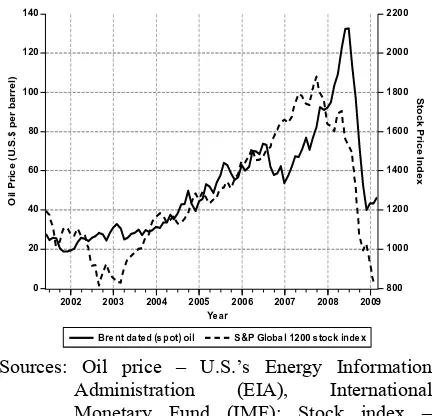
During the late 2000s, global stock trading was exposed to a series of critical conditions, such as high commodity prices and the U.S. financial crisis. Worldwide stocks’ performance was closely paralleled with unusually sharp price increases and a subsequent strong reverse in globally traded raw commodities, including crude oil (see Figure 1). However, does this happen in a particular and noteworthy way, or it is just a coincidence and has been overstated?
From common sense and the conventional literature, oil price increases may drive stock
Sources: Oil price – U.S.’s Energy Information Administration (EIA), International Monetary Fund (IMF); Stock index – EconStats
Figure 1. Crude Oil Price and Global Composite Stock Index Series during 2000s
As historical counterparts, OPEC’s oil quota increase and Asia-Pacific’s lower oil demand made oil prices drop from $20 down to $12 during the 1997 East Asian financial crisis with simultaneous huge capital withdrawals out of the region by panicked investors (Basher and Sadorsky, 2006; Asmar and Brahmana, 2013). Even though a serious oil shortage did not happen, oil prices moved in an increasing upward trend after the 2001 attacks in the U.S. (Hamilton, 2009; Williams, 2008) while in the meantime there was a global economic expan-sion from 2002 to 2006 (Guell, 2008a; Williams, 2008).
Following the major oil price shocks of the 1970s an extensive catalogue of literature has investigated the link between oil prices and economic activities. For instance, Hamilton (1983) argues that oil price shocks contributed to the US recession. Cologni and Manera (2008), Kilian (2008), Park and Ratti (2008) have strengthened this conclusion when they found similar results in developed countries. The second wave of the oil price’s effect on econo-mic activity continues with its impact on stock markets. For instance, Jones and Kaul (1996) find that oil price increases in the post war period have had a significantly negative impact on the US stock market. Sadorsky (1999) reports
the same conclusion with a little addition, which is that the magnitude of the effect may have increased since the mid 1980s. Conversely, Huang et al. (1996) has not found a significant contribution by oil prices on US stock returns. Meanwhile, Ciner (2001) documents the non-linear relationship between oil’s price and stock markets. Note that those studies were conducted at a time when oil prices kept increasing. It is rare to find research investigating an oil price shock with a downward trend, as we see today.
In this research, we argue that the trans-mission of oil shocks with an upward trend might be different to those with a downward trend. There is a possibility of interdependence among stock markets, and to verify the inter-dependence among regional stock markets as a result of the transmission of the oil shock’s impact. The potential wide spreading effects of oil prices in the region is sought to be negated with the use of time-varying correlation modelling across stock markets during the oil price shock. The spreading effect would be evidenced if non-direct oil-unaffected stock markets are significantly correlated with those direct oil-affected markets, by having the same direction of movement during oil price shocks.
Further, this present analysis aims to examine the stock markets’ behaviour during global oil price shocks (sudden changes). A multivariate model, where data changes series as information is conditioned with negative (decreasing) separated shocks and as the risk factors and changes in the fluctuations (volatility) are built into the model to discover this possibly wide interdependence relation.
The current research has important implications for regional investment portfolios. When building up an international investment portfolio, investment analysis involves deciding which composite stocks to include, given the global oil impact, or how to prevent or minimize the negative impacts from the stock markets’ integration. Since the spread effect indicates the possibility of the various stock markets’ como-vement, as caused by the oil price shock, the potential for a portfolio’s risk-diversification into East Asian stock markets would be worth
0 20 40 60 80 100 120 140
800 1000 1200 1400 1600 1800 2000 2200
2002 2003 2004 2005 2006 2007 2008 2009
Brent dated (spot) oil S&P Global 1200 stock index
O
il
P
ri
c
e
(
U
.S
.$
p
e
r
b
a
rr
e
l)
S
to
c
k
P
ri
c
e
In
d
e
x
the risk, if the spread effect is weak or not found. However, the portfolio has to be managed more efficiently if oil price is found to be a contagious factor among stock markets. Or if the diversifi-cation’s benefit is not found when all the stock markets are simultaneously affected by an oil shock, what steps can be suggested?
PREVIOUS STUDIES
Earlier studies have focused on the concept of identifying the best individual stock for investment. The benefit from the international diversification of investments is found in the risk diversification strategy, as developed by Harry Markowitz and James Tobin in the 1950s, by using mean-variance (return-risk) estimates of portfolios (Gagnon & Karolyi, 2006; Engle, 2004). Their optimization strategy is still in use to construct portfolios with the largest stock returns for an acceptable risk. However, the correlation between nations’ stock market indexes was found to be more justifiable after the October 1987 stock crash, due to the more integrated markets with advanced systems technology, more liberalized capital flows, and more cross-national listed companies (Gagnon & Karolyi, 2006).
The shock and volatility spill-over/trans-mission among financial markets for stocks and other instruments across nations is a revolu-tionary subject for international finance. A common and global factor such as an oil price shock can be transmitted across stock markets, due to the fundamental trade channel, such as the large stock trading flow between the markets, and the degree of integration and liberalization of the markets (Yung et al., 2000). The world and regional economies have fast become globalized and integrated, not only due to the liberalization of the financial markets, but also due to the development of fast and efficient information and communications technology. The markets’ comovement may also be due to its unchecked liquidity flow which unknowingly lets investors withdraw funds from many regional markets. Forbes and Rigobon (2001) further customize the contagion factor as being crisis-based, in which a crisis in one national
market can coordinate investors’ expectations, leading them to shift their investment from another good market.
Increased interdependence or linkages among the stock markets in a world of high capital mobility may imply the risk of cross-border contagion, in particular within regions (Jung, 2008). Thus, financial instability in one nation can be transmitted to neighbouring nations more rapidly during times of oil crisis or shocks. Macro shocks directly affect all the markets and economies, whereas micro shocks spread throughout several markets via contagion (Ray, 2010). While every market is vulnerable to macro oil shocks, regional highly connected markets are also vulnerable to micro oil shocks, and thus are exposed to the aggregated risk.
DATA AND METHODOLOGY
This research uses daily data of oil prices (both the Brent Oil Price and WTI Oil Price) and the stock market returns of Asian stock markets over the period from 1999 to 2014. The oil data are retrieved from the website portal of the Energy Information Administration (EIA). Meanwhile, the stock market returns is a calculated price of the market index taken from Worldscope, available off Thomson Datastream. There are 10 major Asian stock markets, comprising of five from the Southeast Asia (SEA) and five from the Northeast Asia (NEA) sub-regions. There are five total oil importers (the Philippines, Hong Kong SAR, Taiwan, South Korea, and Japan), four net oil importers (Indonesia, Singapore, Thailand, and China), and one net oil exporter (Malaysia).
The MGARCH model is an extension of the univariate GARCH model, allowing simulta-neous modelling of the conditional variances of several series. It can also be used to investigate whether the volatility of an asset (e.g. oil price) can be indirectly transmitted to other markets (e.g. stocks) through the first affected market (i.e. stock), or in other words the volatility spillover/contagion effect (Silvennoinen & Terasvirta, 2009; Laurent, 2010).
In the most basic algebraic expression, let
{
��} be the price/index series of any one asset, holding the asset for one period from date� − 1
to date t would result in a returns percentage of:
�(= 100 ∗ (ln �(− ln �(/0) (1)
The time-subscript operator written as (∙)( is used to indicate a conditional moment. By using the time series regression of Box-Jenkins’s 1970s Autoregressive Moving Average (ARMA) while inserting oil price changes as an exoge-nous explanatory variable into the equation, a general stationary ARMAX(1,0,1) bivariate regression process would be obtained:
�3(456,(= � + ��3(456,(/0+ ��4<=,(+ �( (2) As the usual proxy for shock/innovation from econometrics literature, the random/ stochastic regressed series {�(} here is mathematically the deviation among stock returns �3(456,( and its one day lagged �3(456,(/0, oil price changes �4<=,( , and their long-run constant reverting �:
�( = �3(456,(− � − ��3(456,(/0− ��4<=,( (3) Although �( are serially uncorrelated with a conditional zero mean (central expectation) of:
� �( �(/0 = � �( �(/0,�(/B, … , �B, �0
= 0 , [�0≠ �B] , (4) They are dependent (self-regress) from one period to the next in terms of their conditional variances �(B:
��� �( �(/0 = ��� �( �(/0,�(/B, … , �B, �0
= � �(�( �(/0 = � �(B �(/0
= � �(B�(B�(/0
= �(B� �(B�(/0
= �(B��� �( �(/0 = �(B 1
= �(B ,
�
(= �
(∙ �
(⇔ �
(B= �
(B∙ �
(B,
��� �
(�
(/0= 1 , �
(�
(/0~� 0, �
(B,
(5)
Where ��� ∙ ∙ is the conditional variance operator, squared shock �(B is the proxy of historical volatility, �( is the standardized �( (by conditional standard deviation �) which has a constant variance, and P is the {�(}’s conditional probability distribution with a conditional zero mean and non-constant variance.The Threshold GARCH (TGARCH) model which has been independently proposed by Glosten-Jagannathan-Runkle in 1993 and Zakoian in 1994 is referred to, to specify the asymmetry negative shock effect. GARCH has the advantage of using smaller lagged orders of historical information (Engle, 2004), in particular the TGARCH(1,1) volatility model, which is sufficient in practice as specified as follows:
�(B = � + ��(/0B + ��(/0�(/0B + ��(/0B (6) Where �(Bis the conditional variances, squared shock �(B is the proxy of historical volatility, and �( is the dummy variable for the sign of �(. When the past shock is negative, which implies a sudden decrease (�(/0< 0), then �(/0= 1, and the model equation would be:
�(B = � + ��(/0B + ��(/0B + ��(/0B (7) With � + � ≥ 0, otherwise �(/0 ≥ 0 ⇒ �(/0= 0 , which would reduce to a linear GARCH(1,1):
Contemporaneous cross-correlation among oil-stock regressed shocks �( can entail the interdependence among several series. For investigating co-movement patterns among several stock markets due to the global oil price factor, the �( from each of the above oil-stock bivariate regressions are de-volatilized or standardized (by the conditional standard deviation �():
�( = �(∙ �( ⟺ �( = TU
VU (9) �( is the random standardized shocks which are independent and identically t-distributed (i.i.t-d.) with a conditional zero mean and normalized to a constant value-one variance:
� �( �(/0 = � �( �(/0,�(/B, … , �B, �0 = 0 ...(10)
��� �
(�
(/0= � �
(�
(�
(/0= � �
(�
(�
(/0�
(/0,�
(/B�
(/B, … , �
B�
B, �
0�
0= � �
(B�
(/0= � �
(B�
(/0B, �
(/BB, … , �
BB, �
0B= 1
�
(~����(0, 1)
Thus, each oil-stock’s own standardized volati-lity is set as a non-AR and constant, in order to enhance the significance of the cross-series correlation.
In a multivariate form of the N series, the {�(} and {�(} can be written in vector as (Laurent, 2010; Jondeau et al., 2007):
��= ������
� �
∙ �� ⇔ �� = ������ /� �
∙ �� (11) With:
��= �0,( �B,( ⋮ �c,( �×�
, ��=
�0,( �B,( ⋮ �c,( �×�
,
�����
�� �= ���� ℎ
0,0,(, ℎ
B,B,(, … , ℎ
c,c,( 0/B= ���� �
0,(B, �
B,(B, … , �
c,(B 0/B= ���� �
0,(, �
B,(, … , �
c,(=
�
0,(0
0
…
0
0
�
B,(0
…
0
0
⋮
0
0
⋮
0
�
i,(⋱
…
⋱
⋱
0
⋮
0
�
c,( ��,
�����
�/� �=
�
0,(0
0
…
0
0
�
B,(0
…
0
0
⋮
0
0
⋮
0
�
i,(⋱
…
⋱
⋱
0
⋮
0
�
c,( ��/0
��� �
��
�/�= � �
��
�′
�
�/�= �
�
0,(�
B,(⋮
�
c,( c×0�
0,(�
B,(…
�
c,( 0×c�
�/�=
ℎ
0,0,(ℎ
0,B,(…
ℎ
0,c,(ℎ
B,0,(⋮
ℎ
c,0,(ℎ
B,B,(⋮
ℎ
c,B,(…
⋱
…
ℎ
B,c,(⋮
ℎ
c,c,( ��= �
��
�= �����
� �/�∙ �
�∙ �����
� �/�=
�
0,(0
0
…
0
0
�
B,(0
…
0
0
⋮
0
0
⋮
0
�
i,(⋱
…
⋱
⋱
0
⋮
0
�
c,( �×�∙ �
�∙
�
0,(0
0
…
0
0
�
B,(0
…
0
0
⋮
0
0
⋮
0
�
i,(⋱
…
⋱
⋱
0
⋮
0
�
c,( �×���� ∙ ∙ is the conditional covariance operator,
ℎ( are ��’s covariance elements, and ������ �/�
is the diagonal matrix with conditional standard deviations �<,( is actually the case of ℎ<,<,( since two correlated {�(} are the same (between i and i series) on the i-th diagonal.
The time-varying �� of �� is actually the standardized �� of ��. Thus, the �� is further established by decomposing itself into ������/� �and ��, with �� as the positive definite conditional covariance matrix of �� (Thastrom, 2008):
��� �� ��/� = � ����ʹ��/� =
� �0,( �B,( ⋮ �c,( c×0
�0,( �B,( … �c,( 0×c ��/� =
�0,0,( �0,B,( … �0,c,( �B,0,(
⋮ �c,0,(
�B,B,( ⋮ �c,B,(
… ⋱ …
�B,c,( ⋮
�c,c,( c×c
= �� (12)
To ensure a lesser number and reasonable value of the parameters in the conditional correlation model’s likelihood function, the
intercept of �� is applied here as correlation targeting for 1 − A − � � with the implication it is expressed in terms of its own long-run unconditional positive definite constant matrix � and two correlation persistence parameters A and B (Laurent, 2010). In Engle-Sheppard’s (2001) Dynamic Conditional Correlation (DCC) model of both adequate one lagged orders DCC(1,1), �� is estimated as:
�� = 1 − A − � � + � ��/���/�ʹ + ���/�
= 1 − A − � � + � ������� �∙ ��/���/�ʹ∙
������� � + ���/� , � = � ����ʹ =
0
y ����ʹ y
(z0 (13)
{�(} are the same (between the i and i series) on the i-th diagonal:
������� �= ���� �0,0,( , �B,B,( , … , �c,c,( 0 B
= ���� �0,(B , �B,(B , … , �c,(B | }
= ���� �0,( , �B,( , … , �c,(
=
�0,( 0 0 … 0
0 �B,( 0 … 0
0 ⋮ 0
0 ⋮ 0
�i,( ⋱ …
⋱ ⋱ 0
⋮ 0 �c,( c×c
(14)
As the element of �� , the conditional covariance �<,~,( of �( among any two series can be expressed by a mean reverting approach:
�
<,~,(= ��� �
<,(, �
~,(�
(/0= � �
<,(�
~,(�
(/0= �
<,~1 − � − �
+ ��
<,(/0�
~,(/0+ ��
<,~,(/0Where �<,~ is the unconditional correlation which is also the average of �<,~,(. Since �� does not have ones on its diagonal and does not generally produce a valid correlation matrix (Silvennoinen & Terasvirta, 2009), it needs to be rescaled to a proper ��. The �� with �(� − 1)/2 pair-wise parameters �<,~,( is decomposed as:
��= ���� �� ��/� = ������/� ���������/� �=
�0,( 0 0 … 0
0 �B,( 0 … 0
0 ⋮ 0
0 ⋮ 0
�i,( ⋱ …
⋱ ⋱ 0
⋮ 0 �c,( �×�
/0
∙
�0,0,( �0,B,( … �0,c,( �B,0,(
⋮ �c,0,(
�B,B,( ⋮ �c,B,(
… ⋱ …
�B,c,( ⋮
�c,c,( �×� ∙
�0,( 0 0 … 0
0 �B,( 0 … 0
0 ⋮ 0
0 ⋮ 0
�i,( ⋱ …
⋱ ⋱ 0
⋮ 0 �c,( �×�
/0
=
1 �0,B,( �0,i,( … �0,c,( �B,0,( 1 �B,i,( … �B,c,( �i,0,(
⋮ �c,0,(
�i,B,( ⋮ �c,B,(
1 ⋱ …
⋱ ⋱ �c,c/0,(
⋮ �c/0,c,(
1 c×c
, (15)
�����
�= �
0,0,(, �
B,B,(, … , �
c,c,(= 1 ,
0 < �
<,~,(< 1 ,
��is reported as being lower-triangular and symmetric because �<,~,( = �~,<,( with the diagonal equal to one, and ������/� � is a normalization matrix to guarantee �� as a conditional correlation matrix (Tsay, 2005). The positive definite �� would have correlation parameters valued at one on its diagonal since the correlation of any �( with itself, and the diverse parameters �<,~,( in the range of absolute value −1 < �<,~,(< 1 on the off-diagonal as long as �� is positively definite. As the element of �� , the particular conditional correlation parameter �<,~,( would be:
�<,~,(= ���� �<,( , �~,( �(/0
= ��� �<,( , �~,( �(/0
��� �<,( �(/0 ∙ ��� �~,( �(/0
= � �<,(�~,( �(/0
� �<,(�<,( �(/0 ∙ � �~,(�~,( �(/0
= ‡ Tˆ,UT‰,UŠU‹|
‡ Tˆ,U} ŠU‹| ∙‡ T‰,U} ŠU‹|
= Œˆ,‰,U
Œˆ,ˆ,UŒ‰,‰,U
= Œˆ,‰,U
Vˆ,U}V‰,U}
=
Œˆ,‰0/•/Ž ••Tˆ,U‹|T‰,U‹|•ŽŒˆ,‰,U‹|
Œˆ,ˆ0/•/Ž ••Tˆ,U‹|} •ŽŒˆ,ˆ,U‹| Œ‰,‰0/•/Ž ••T‰,U‹|} •ŽŒ‰,‰,U‹|
=
Œˆ,‰0/•/Ž ••Tˆ,U‹|T‰,U‹|•ŽŒˆ,‰,U‹|
Vˆ}0/•/Ž ••Tˆ,U‹|} •ŽVˆ,U‹|} V‰} 0/•/Ž ••T‰,U‹|} •ŽV‰,U‹|}
(16)
���� ∙ ∙ is the conditional correlation
operator. Parameters A and B can be tested respectively to check whether the N series are empirically imposing time-varying conditional correlations. Modelling any �( would give consistent estimates of parameters A and B. If � , � = 0, the conditional correlation would be constant (Thastrom, 2008).
It is not easy to visualize a long series of the big correlation matrix, although it holds an interpretive value. Elton and Gruber even proposed the averaging of pair-wise correlations in 1973 in order to reduce the estimation noise and deliver better assets’ allocations and portfolio analysis (Engle & Kelly, 2008). Thus, the time-varying conditional equicorrelation where all assets share a pair-wise correlation equal at each time, but varying over time is additionally modelled here. Equicorrelation assumptions allow the estimation of a large arbitrarily sized correlation matrix with ease (Engle & Kelly, 2008). In equicorrelation, several {�(} series may share the same correlation at the same time while being allowed to vary over time. Attaining a general average result of the correlations for direct interpretation is the main motivation behind the further use of equicorrelation. Another feature of equicorre-lation would be its advantage of having nume-rical stability for the MLE of the parameters’ convergence (Thastrom, 2008).
ℝ� is an equicorrelation matrix with parameters valued 1 on the diagonal and equal to �( on all off-diagonals (Engle & Kelly, 2008):
ℝ�= 1 − �( � + �(��ʹ= 1 − �( � + �(� = 1 − �(
1 0 0 … 0
0 1 0 … 0
0 ⋮ 0
0 ⋮ 0
1 ⋱ …
⋱ ⋱ 0
⋮ 0
1 ��
+
�( 1 1 ⋮
1 c×0
1 1 … 10×c = 1 − �(
1 0 0 … 0
0 1 0 … 0
0 ⋮ 0
0 ⋮ 0
1 ⋱ …
⋱ ⋱ 0
⋮ 0
1 ��
+ �(
1 1 … 1
1 ⋮ 1
1 ⋮ 1
… ⋱ …
1 ⋮
1 c×c
=
1 �( �( … �(
�( 1 �( … �(
�( ⋮ �(
�( ⋮ �(
1 ⋱ …
⋱ ⋱ �(
⋮ �(
1 c×c
Where �( is the scalar equicorrelation averaged from all the pair-wise correlations, � denotes the identity matrix, � is the vector of ones, and � is the matrix of ones. Only one equicorrelation for each time � is recorded, thus one time-varying conditional equicorrelation series {�(} is generated similar to one lagged order of ARMA(1,1) (Christoffersen et al., 2010):
�( = 1 − � − � � + ��(/0+ ��(/0 (18)
With � and � as time-varying parameters, �( is the average correlation between different �( averaged by �(� − 1) quantities (of pair-wise correlations) as:
�( =
1
� � − 1 �<,~,(
<™~
= 0 c(c/0)
Œˆ,‰,U
Œˆ,ˆ,UŒ‰,‰,U
<™~ (19)
The ℝ� and �( are positive and definite if and only if (Engle & Kelly, 2008):
− 0
c/0< �( < 1 (20)
Even if �� are not equicorrelated, the model would reduce to the previous mentioned �(� − 1)/2 quantities of the pair-wise correlation parameters.
The cross-series correlation model under the conditional multivariate Student’s t−distribution is implemented here. It is a distribution for capturing dependency among the distribution tails of �� (Jondeau et al., 2007). Under this t -distribution, the �� is obtained under conditional joint normality, and then simply tested by the Student’s t-test on the probability assumption (Gonzalez-Rivera & Yoldas, 2010). Specifically, the degrees of freedom (d.f.) parameters for all the pair-wise correlations �( are first estimated separately, then an average of all the individual estimates is considered for the distributional specification in the multivariate model (Gonzalez-Rivera & Yoldas, 2010).
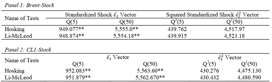
In order to check the adequacy of the fitted multivariate model with changing conditional covariance over time, the cross-series ACV property of vector �� and ��� matrices can be defined. In particular, the Hosking’s and
Li-McLeod’s multi-equation portmanteau Q-tests are performed to check ACV property for the validity of several series’ correlations and to ensure there is no remaining heteroskedasticity in the variance and covariance of ��� . The simultaneous correlation of �� can be captured by the model when assuming ��� to obey cross-series non-autocovariated moment conditions (Laurent, 2010):
��� �
���
�/�= � �
���
��′
�
�/�= � �0,(B �B,(B ⋮ �c,(B
c×0
�0,(B �B,(B … �c,(B 0×c ��/�
=
1 0 0 … 0
0 1 0 … 0
0 ⋮ 0
0 ⋮ 0
1 ⋱ …
⋱ ⋱ 0
⋮ 0
1 ��
,
��� �
<,(B, �
~,(B�
(/0= � �
<,(B�
~,(B�
(/0= 0 � ≠ � ,
��� �
<,(B, �
~,(/6B�
(/0= � �
<,(B�
~,(/6B�
(/0= 0 � > 0 ,
While allowing �� to be autocovariated: ��� �� ��/� = � ����′��/�
= � �0,( �B,( ⋮ �c,( c×0
�0,( �B,( … �c,( 0×c ��/�
=
�0,0,( �0,B,( … �0,c,( �B,0,(
⋮ �c,0,(
�B,B,( ⋮ �c,B,(
… ⋱ …
�B,c,( ⋮
�c,c,( c×c
��� �<,( , �~,( �(/0 = � �<,(�~,( �(/0
The model has been carefully written for the explanation of oil-stock regressions and cross series contemporaneous correlations. The important advantage of this three-step model would be the estimation of only a very few parameters in a sequential fashion. First, all individual stock market returns are conditionally made regressive to the oil price change for checking the effect parameters. Then, each regressed shock is squared and the (negatively) nonlinear threshold for time-varying volatility/risk is estimated. Lastly, the regressed shocks are standardized and the time-varying conditional correlation matrix is estimated. A thorough examination of the model can be supported with the types of diagnostic checks used on regressed shocks.
RESULTS
Descriptive Return Statistics
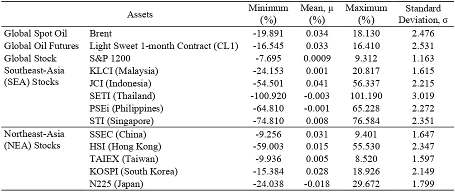
Table 1 shows the descriptive statistics of the observed data particular to each test between two oil prices and one global composite stock (the S&P 1200). The unconditional mean/averages of all the returns are very small, with some stock market returns even being negative. Indonesia’s composite stock (the JCI) earned the highest
mean at 0.04%, while Japan’s N225 earned the lowest at −0.018%.
The two global crude oil returns seem to move in unison, but the 1-month oil futures (CL1) rates appear to be more volatile. CL1 are more volatile than the spot oil (Brent) as indicated by a higher unconditional standard deviation (σ: 2.53 > 2.476), although both of them earned equal returns at 0.03%, which is as high as some of the national composite stocks such as China (SSEC) and South Korea (KOSPI). Only Thai stocks (SETI) swing the most at σ = 3.0, whereas some are more stable at a low σ value of around 1.0 to 2.0.
Return Distribution Statistics
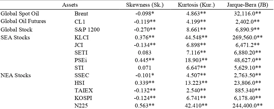
[image:10.595.70.525.535.727.2]The unconditional normality statistics are shown in Table 2. The parameter/coefficient of skewness (Sk) is nil (0) for a symmetric normal distribution. The positive or negative of Sk would directly entail whether those extremes are boom or crash. Both types of oil are uncondi-tionally negatively skewed, but oil futures have more negative extremes (Sk: −0.119 > −0.098). Global stock is highly negatively skewed. For those national stocks which are negatively skewed, their Sk’s are little more than −0.1. Whereas the positively skewed stocks have higher Sk values spanning from 0.33 to 0.56.
Table 1. Unconditional Descriptive Statistics of Daily Oil Price Change and Composite Stock Returns
Assets Minimum
(%)
Mean, µ
(%)
Maximum (%)
Standard Deviation, σ
Global Spot Oil Brent -19.891 0.034 18.130 2.476 Global Oil Futures Light Sweet 1-month Contract (CL1) -16.545 0.033 16.410 2.531 Global Stock S&P 1200 -7.695 0.0009 9.312 1.163 Southeast-Asia
(SEA) Stocks
KLCI (Malaysia) -24.153 0.001 20.817 1.615 JCI (Indonesia) -54.501 0.041 56.337 2.215 SETI (Thailand) -100.920 -0.003 101.190 3.019 PSEi (Philippines) -64.810 -0.001 65.228 2.272 STI (Singapore) -74.810 0.008 76.584 2.351 Northeast-Asia
(NEA) Stocks
SSEC (China) -9.256 0.031 9.401 1.647
HSI (Hong Kong) -59.003 0.015 55.530 2.347 TAIEX (Taiwan) -9.936 0.005 8.520 1.597 KOSPI (South Korea) -15.384 0.028 18.926 2.149 N225 (Japan) -24.038 -0.018 29.672 1.799 Source: Data Calculated from Energy Information Administration database
Table 2. Unconditional Normality of Shock/Residual Statistics
Assets Skewness (Sk.) Kurtosis (Kur.) Jarque-Bera (JB)
Global Spot Oil Brent -0.098* 4.863** 32,116.0**
Global Oil Futures CL1 -0.119** 4.199** 2,402.0** Global Stock S&P 1200 -0.270** 8.661** 6,890.9**
SEA Stocks KLCI 0.376** 44.548** 269,560.0**
JCI -0.134** 6.898** 6,471.2**
SETI 0.083 7.116** 6,880.20**
PSEi 0.445** 18.903** 48,627.0**
STI 0.071 6.647** 5,629.10**
NEA Stocks SSEC -0.101* 4.507** 2,763.50**
HSI 0.339** 13.223** 23,806.0**
TAIEX -0.132** 2.540** 885.340**
KOSPI -0.124** 6.741** 6,178.40**
N225 0.563** 42.410** 244,400.0**
Source: Data Calculated from Worldscope database. Asterisk (*) - significant at 0.05 t-test probability (p); ** - significant at ≤ 0.01 p
Meanwhile, the kurtosis parameter (Kur) is valued at three for a normal distribution, which is also called the zero value of excess Kur. All assets have a positive excess Kur at Kur > 3, with some stocks even scoring very high Kur values, in the ranges from 13.0 to 19.0 and 42.0 to 45.0. Thus, all the returns’ distributions are heavy-tailed non-normal ones, in which the random returns series tends to contain more extreme values.
Jarque-Bera (JB) statistics for all the assets’ returns, which are based on the simultaneous Sk and Kur parameters, are significant at very small t-test probabilities. This result further confirms that all the returns are sampled from an unconditional non-normal distribution.
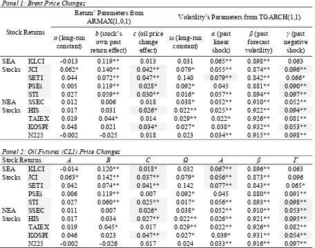
From the column of parameter c in Table 3, price changes for both types of global oil are found to be positively regressed on global and all East Asian stock market returns, denoting that the composite stock indexes are mostly moving in the same direction, in response to the oil price trend. All composite stock markets except the N225 and Taiwan (TAIEX) are significantly affected by either the spot oil or oil futures prices, although the effects of parameter c are small, in a range from 0.02 to 0.05.
From those significant oil-stock relations, most regressed shocks
�
( from the regression ofBrent toward each national stock are found to be
significantly negative in affecting volatility, meaning that the spot price of oil decreases rather than increases in its effect, as a consequence it drives the stock markets’ volatility and downward (poor) performance of stocks. The column
�
in Table 1 implies the parameter and significance of the negative shock.For
�
( regressed from CL1 toward each stock, SEA’s stock markets are found to have a mostly linear reaction toward shock (see�
column in Panel 2 of Table 1), meaning that the positive and negative effects are significantly equal and there are no asymmetric negative effects. Meanwhile, CL1 is found to have a significant negative shock effect on global and NEA’s stocks.
Conditional correlations among oil’s directly affected and unaffected composite stocks are computed in order to find out whether oil has contagious and spreading effects. The condi-tional correlation matrix
�
� of the selected standard oil-stock regressed shocks�
( is reported as a symmetrical and lower-triangular matrix with its diagonal equal to one. Each cell records the conditional correlation parameter�
(between the two relevant
�
(s. Since there is onlyone
�
( between�
<,( and�
~,(, regardless of theTable 3. Parameters Estimation from Oil-Stock’s Conditional Regressed Returns and Volatility Model
Panel 1: Brent Price Changes
Stock Returns
Return’ Parameters from
ARMAX(1,0,1) Volatility’s Parameters from TGARCH(1,1)
a (long-run constant)
b (stock’s own past return effect)
c (oil price change effect)
ω (long-run constant)
α (past linear shock)
β (past forecast volatility)
γ (past negative
shock) SEA
Stocks
KLCI -0.013 0.119** 0.013 0.031 0.065** 0.898** 0.063 JCI 0.062* 0.140** 0.042** 0.079* 0.055** 0.874** 0.096** SETI 0.044 0.072** 0.047** 0.140 0.079** 0.842** 0.066* PSEi 0.005 0.119** 0.028* 0.092* 0.045 0.881** 0.090** STI 0.027 0.059** 0.030** 0.016* 0.057** 0.894** 0.097** NEA
Stocks
SSEC 0.012 0.006 0.018 0.038* 0.052** 0.910** 0.052** HIS 0.017 0.031 0.026* 0.022** 0.025** 0.922** 0.094** TAIEX 0.019 0.044* 0.014 0.029** 0.022* 0.926** 0.081** KOSPI 0.048 0.021 0.034* 0.027* 0.038* 0.932** 0.053** N225 -0.002 -0.025 0.018 0.023 0.034** 0.915** 0.098**
Panel 2: Oil Futures (CL1) Price Changes
Stock Returns A B C Ω Α β Γ
SEA Stocks
KLCI -0.014 0.120** 0.018* 0.032 0.067** 0.896** 0.063 JCI 0.063* 0.142** 0.037** 0.079* 0.056** 0.873** 0.096 SETI 0.042 0.074** 0.041** 0.142 0.077** 0.843** 0.065* PSEi 0.006 0.119** 0.007 0.092* 0.045 0.880** 0.091** STI 0.027 0.060** 0.025** 0.017* 0.056** 0.893** 0.098** NEA
Stocks
SSEC 0.011 0.007 0.026* 0.038* 0.052** 0.910** 0.053** HIS 0.017 0.034 0.027** 0.022** 0.026** 0.921** 0.095** TAIEX 0.019 0.045* 0.017 0.029** 0.022** 0.926** 0.082** KOSPI 0.046 0.023 0.047** 0.027* 0.039* 0.931** 0.054** N225 -0.002 -0.026 0.017 0.024 0.033** 0.916** 0.097** Notes: * - significant at 0.05 t-test probability (p); ** - significant at ≤ 0.01 p
There are two global oil prices and ten stock markets in the current sample of our contagion analysis. The conditional correlations are counted separately in two matrixes, the first being between spot oil (Brent) and stocks, while the second is between oil futures (CL1) and stocks. From the ten (10)
�
(s generated from theten oil-stock bivariate regressions, only
0œ 0œ/0 B
=
0œ • B
=
•œ
B
= 45
pair-wise�
( from�
� are examined. This can be further detail counted as10×10 = 100
pair-wise�
( of a 10th dimension squared�
�, minus the 10 units ofdiagonal one and the repeated half triangular
�
(,thus as a consequence 0œœ/0œ
B
=
•œB
= 45
pair-wise
�
( are the�
( between different�
( thatwould be observed.
�
( is a correlation parameter in terms of the time series, thus only the averageof the
�
( series, denoted as�
, would be shownin Table 4 and Table 5. The two tables of each 45 pair-wise
�
s are tabulated by being further separated into three groups of�
s, there are�
s between any two oil-affected stocks,�
s between oil-affected and oil-unaffected stocks, and lastly the�
s between two oil-unaffected stocks. The first two mentioned groups of�
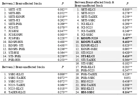
s are the targeted results for oil’s contagious factor effect investigated by this current research.Table 3 shows that five out of the six Brent-affected national composite stocks are found to be significant, and having a high
�
among each other. The Philippines’ stock market (PSEi) is omitted, as it is weakly correlated with the others, as indicated by the lowest range of�
(�
Table 4. 45 Pair-Wise Conditional Correlation Parameters (ρ) among 10 Standardized Oil-Stock Regressed Shocks (Brent - Stocks)
Between 2 Brent-affected Stocks Ρ Between Brent-affected Stock &
Brent-unaffected Stock Ρ
1. SETI -STI 0.382** 1. SETI-KLCI 0.333**
2. SETI-HIS 0.352** 2. SETI-N225 0.276**
3. SETI-KOSPI 0.319** 3. SETI-TAIEX 0.259**
4. SETI-JCI 0.292** 4. SETI-SSEC 0.076**
5. SETI-PSEi 0.209** 5. JCI-KLCI 0.298**
6. JCI-STI 0.370** 6. JCI-N225 0.267**
7. JCI-HSI 0.347** 7. JCI-TAIEX 0.249**
8. JCI-KOSPI 0.303** 8. JCI-SSEC 0.054*
9. JCI-PSEi 0.228** 9. KOSPI-N225 0.487**
10. KOSPI-HIS 0.488** 10. KOSPI-TAIEX 0.453**
11. KOSPI- STI 0.438** 11. KOSPI-KLCI 0.323**
12. KOSPI- PSEi 0.236** 12. KOSPI-SSEC 0.095**
13. STI-HSI 0.564** 13. STI-N225 0.420**
14. STI- PSEi 0.259** 14. STI-KLCI 0.415**
15. PSEi-HIS 0.253** 15. STI-TAIEX 0.364**
Between 2 Brent-unaffected Stocks Ρ
16. STI-SSEC 0.102** 17. PSEi-KLCI 0.285** 18. PSEi-N225 0.247**
1. SSEC-KLCI 0.086** 19. PSEi-TAIEX 0.229**
2. SSEC-TAIEX 0.072** 20. PSEi-SSEC 0.051
3. SSEC-N225 0.072** 21. HSI-N225 0.456**
4. N225-TAIEX 0.368** 22. HSI-TAIEX 0.388**
5. N225-KLCI 0.318** 23. HSI-KLCI 0.376**
6. TAIEX-KLCI 0.273** 24. HSI-SSEC 0.154**
Notes: * - significant at 0.05 t-test probability (p); ** - significant at ≤ 0.01 p Four Brent-unaffected composite stocks are
found significant in influencing those Brent-affected stocks, but only three are correlated with a high
�
(excepting the SSEC). Three Brent-affected stocks from the KOSPI, Singapore (STI), and Hong Kong (HSI) are found to generally have a high�
with three Brent-unaffected stocks from the N225, TAIEX, and Malaysia (KLCI).Table 5 shows that there are five CL1-affected stocks which are highly and significantly correlated with each other. By excluding the weak CL1-affected KLCI and the weak correlated SSEC, those five CL1-affected stocks are KOSPI, SETI, JCI, HSI, and STI.
Meanwhile, there are two out of three CL1-unaffected national stocks which are found to be stronger and significantly correlated to those CL1-affected stocks. These are the TAIEX and N225, (but not the PSEi), the two CL1-unaffected stocks which are strong and
significantly correlated with the three CL1-affected stocks – KOSPI, HSI, and STI.
Table 5. 45 Pair-Wise Conditional Correlation Parameters (ρ) among 10 Standardized Oil-Stock Regressed Shocks (Oil Futures/CL1 - Stocks)
Between 2 CL1-affected Stocks Ρ Between affected Stock &
CL1-unaffected Stock Ρ
1. KOSPI-HIS 0.486** 1. KOSPI-N225 0.487**
2. KOSPI-STI 0.436** 2. KOSPI-TAIEX 0.452**
3. KOSPI-KLCI 0.322** 3. KOSPI-PSEi 0.237**
4. KOSPI-SETI 0.318** 4. SETI-N225 0.276**
5. KOSPI-JCI 0.302** 5. SETI-TAIEX 0.257**
6. KOSPI-SSEC 0.094** 6. SETI-PSEi 0.212**
7. SETI-STI 0.381** 7. JCI-N225 0.266**
8. SETI-KLCI 0.335** 8. JCI-TAIEX 0.247**
9. SETI-HIS 0.351** 9. JCI-PSEi 0.229**
10. SETI-JCI 0.291** 10. HSI-N225 0.455**
11. SETI-SSEC 0.076** 11. HSI-TAIEX 0.386**
12. JCI-STI 0.369** 12. HSI-PSEi 0.253**
13. JCI-HIS 0.345** 13. SSEC-TAIEX 0.071**
14. JCI-KLCI 0.299** 14. SSEC-N225 0.071**
15. JCI-SSEC 0.053* 15. SSEC-PSEi 0.052
16. HSI-STI 0.564** 16. STI-N225 0.419**
17. HSI-KLCI 0.376** 17. STI-TAIEX 0.363**
18. HSI-SSEC 0.153** 18. STI-PSEi 0.259**
19. SSEC-STI 0.102** 19. KLCI-N225 0.318**
20. SSEC-KLCI 0.086** 20. KLCI-PSEi 0.288**
21. STI-KLCI 0.416** 21. KLCI-TAIEX 0.273**
Between 2 CL1-unaffected Stocks Ρ
1. TAIEX-PSEi 0.228**
2. TAIEX-N225 0.368**
3. N225-PSEi 0.247**
Notes: * - significant at 0.05 t-test probability (p); ** - significant at ≤ 0.01 p
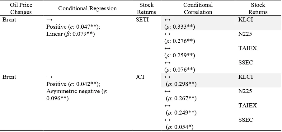
Table 6. Results of Significant Oil-Stock Conditional Bivariate Regression and Conditional Multi-variate Correlation among Standardized Oil-Stock Regressed Shocks (Brent-Stock-Stock) Oil Price
Changes Conditional Regression
Stock Returns
Conditional Correlation
Stock Returns
Brent →
Positive (c: 0.047**); Linear (β: 0.079**)
SETI ↔
(ρ: 0.333**)
KLCI
↔
(ρ: 0.276**)
N225
↔
(ρ: 0.259**)
TAIEX
↔
(ρ: 0.076**)
SSEC
Brent →
Positive (c: 0.042**); Asymmetric negative (γ: 0.096**)
JCI ↔
(ρ: 0.298**)
KLCI
↔
(ρ: 0.267**)
N225
↔
(ρ: 0.249**)
TAIEX
↔
(ρ: 0.054*)
[image:14.595.72.527.119.456.2] [image:14.595.73.526.519.731.2]Brent →
Positive (c: 0.034*); Asymmetric negative (γ: 0.053**)
KOSPI ↔
(ρ: 0.487**)
N225
↔
(ρ: 0.453**)
TAIEX
↔
(ρ: 0.323**)
KLCI
↔
(ρ: 0.095**)
SSEC
Brent →
Positive (c: 0.030**); Asymmetric negative (γ: 0.097**)
STI ↔
(ρ: 0.420**)
N225
↔
(ρ: 0.415**)
KLCI
↔
(ρ: 0.364**)
TAIEX
↔
(ρ: 0.102**)
SSEC
Brent →
Positive (c: 0.028*); Asymmetric negative (γ: 0.090**)
PSEi ↔
(ρ: 0.285**)
KLCI
↔
(ρ: 0.247**)
N225
↔
(ρ: 0.229**)
TAIEX
Brent →
Positive (c: 0.026*); Asymmetric negative (γ: 0.094**)
HIS ↔
(ρ: 0.456**)
N225
↔
(ρ: 0.388**)
TAIEX
↔
(ρ: 0.376**)
KLCI
↔
(ρ: 0.154**)
SSEC Notes: * - significant at 0.05 t-test probability (p); ** - significant at ≤ 0.01 p
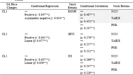
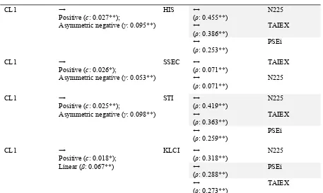
Table 7. Results of Significant Oil-Stock Conditional Bivariate Regression and Conditional Multiva-riate Correlation among Standardized Oil-Stock Regressed Shocks (Oil Futures/CL1-Stock-Stock)
Oil Price
Changes Conditional Regression
Stock
Returns Conditional Correlation Stock Returns
CL1 →
Positive (c: 0.047**);
Asymmetric negative (γ: 0.054**)
KOSPI ↔
(ρ: 0.487**)
N225
↔
(ρ: 0.452**)
TAIEX
↔
(ρ: 0.237**)
PSEi
CL1 →
Positive (c: 0.041**); Linear (β: 0.077**)
SETI ↔
(ρ: 0.276**)
N225
↔
(ρ: 0.257**)
TAIEX
↔
(ρ: 0.212**)
PSEi
CL1 →
Positive (c: 0.037**); Linear (β: 0.056**)
JCI ↔
(ρ: 0.266**)
N225
↔
(ρ: 0.247**)
TAIEX
↔
(ρ: 0.229**)
[image:15.595.70.524.499.754.2]CL1 →
Positive (c: 0.027**);
Asymmetric negative (γ: 0.095**)
HIS ↔
(ρ: 0.455**)
N225
↔
(ρ: 0.386**)
TAIEX
↔
(ρ: 0.253**)
PSEi
CL1 →
Positive (c: 0.026*);
Asymmetric negative (γ: 0.053**)
SSEC ↔
(ρ: 0.071**)
TAIEX
↔
(ρ: 0.071**)
N225
CL1 →
Positive (c: 0.025**);
Asymmetric negative (γ: 0.098**)
STI ↔
(ρ: 0.419**)
N225
↔
(ρ: 0.363**)
TAIEX
↔
(ρ: 0.259**)
PSEi
CL1 →
Positive (c: 0.018*); Linear (β: 0.067**)
KLCI ↔
(ρ: 0.318**)
N225
↔
(ρ: 0.288**)
PSEi
↔
(ρ: 0.273**)
TAIEX Notes: * - significant at 0.05 t-test probability (p); ** - significant at ≤ 0.01 p
Besides, SEA regional stocks such as Malaysia, Thailand, Indonesia, and Philippines are also found to interact closely with each others during oil price shocks, although the Philippines is found to be marginal in the current relationship’s results. They interact mostly in a bidirectional pattern, where which one nation moves closely with one other particular nation, for example both Brent-affected SETI and JCI are correlated with Brent-unaffected KLCI, while CL1-affected SETI and JCI are correlated with CL1-affected PSEi. China’s and the Philippines’ stocks are seen to be working as outsiders since the analysis results of either their oil effect or oil spreading effect within the region are shown to be weak.
[image:16.595.71.528.79.352.2]From the equicorrelation
�
results in Table 8, the overall oil-stock correlation is found to be significant. Thus, all the ten standardized oil-stock regressed shocks (for each spot oil and oil futures sample) can share the same conditional correlation at every specific time which allows them to be different over time. This implies the significant oil factor of stocks’ co-movement is evident and detectable in a time series conditional manner.Table 8. Parameters Estimation from Equi-correlation among 10 Standardized Oil-Stock Regressed Shocks
Parameters Brent-Stocks CL1-Stocks Equicorrelation � 0.315** 0.314** Notes: * - significant at 0.05 t-test probability (p); ** - significant at ≤ 0.01 p
Table 9. Multivariate Portmanteau Q-Statistics for ACV of Standardized Oil-Stock’s Regressed Shocks Vector
Panel 1: Brent-Stock
Name of Tests Standardized Shock �( Vector Squared Standardized Shock �(
B Vector
Q(5) Q(50) Q2(5) Q2(50)
Hosking 949.077** 5,555.0** 439.762 4,517.97
Li-McLeod 948.874** 5,554.18** 439.915 4,523.18
Panel 2: CL1-Stock
Name of Tests �( Vector �(B Vector
Q(5) Q(50) Q2(5) Q2(50)
Hosking 952.083** 5,563.60** 430.276 4,475.130
Li-McLeod 951.879** 5,562.670** 430.432 4,480.590
Notes: ACV - autocovariance
DISCUSSION
The general oil-stock relationship previously had a negative nature due to supply side economics. Since there are positive relationships now being found, especially during the 2000s, the world’s economic growth is seen as the factor making this happen, via the higher demand for fuel to satisfy the needs of industrial production and transportation (Killian & Park, 2007; Gogineni, 2008). A higher demand for oil while the supply remains constant would make oil prices increase. However, the increasing demand for oil by the emerging nations has been partially filled by the developed nations’ environment-friendly policies and reduced consumption of expensive oil (Hamilton, 2009). Therefore, another noteworthy factor would be the expanding of oil futures’ investments that contribute to pushing the oil price higher (UNCTAD, 2009; Master, 2008). Oil consump-tion will continue as long as the buyers can afford to pay its rising price. Stock markets are growing from the indexing of more valuable stocks that were issued by those industries or companies, so oil prices and stock markets can experience positive relations. The Middle-East oil nations’ earnings from the high oil price are being channelled to East Asian economies for investment (JBIC, 2009). That may explain why stock markets in heavy oil consuming nations can positively respond to oil price rises.
Although only a small effect is induced from oil price changes in the current analysis, the stock markets of East Asia are generally being affected, and responding in the same direction of
performance with a 0.3 significant equicorre-lation coefficient. From the daily series of conditional correlation modelling of several oil-stock regressed shocks, significant positive results are found for all the samples. The application of conditional correlation modelling is workable here for the oil risk management of large portfolio investments across nations. Evidence shows that regions are characterized by the presence of changing correlations over time. From conditional correlation’s findings, five East Asian stock markets, consisting of South Korea, Hong Kong, Singapore, Thailand, and Indonesia are found to be directly affected by both spot oil and oil futures prices’ shocks. Whereas all the stock markets’ returns, except for those from China and the Philippines, are highly correlated or their co-movements have increased among themselves and are in the same direction during the oil shocks. As long as oil information can find a path across stock markets, it will affect stock values’ development. Oil price shocks, in particular the negative ones, are found to be a significant driving force for stock markets’ correlations. This result is consistent with the general empirical evidence shown by Gagnon & Karolyi (2006) and Christoffersen (2003) where the correlation between regional markets tends to increase significantly during financial turbulence.
markets become highly integrated when they are exposed to external negative shocks. This can be attributed to the decision they made to open their economies and financial markets to international trade and investment, allowing the international flow of capital. There is an element of risk in integrated stock markets, where the shock from any one of these markets may spillover into the other markets in the same region.
Since these stock markets are interdependent during an oil price negative shock, this suggests that the benefit from a portfolio investment strategy based on diversification is limited within the region. The various stock markets, except for China’s and the Philippines’, are not significant separated assets even though they are from different economies (developed or emerging) and oil activities (oil importing or exporting). Hence, a Chinese or Philippines composite stock can be diversified from the concern of an oil contagious risk toward the portfolio’s investment.
Regional Transmission of Oil Shock’s Effect
The stock markets’ shocks are attributed to the regional transmission of oil shocks. In current research of the conditional correlation analysis, South Korea, Hong Kong, and Singa-pore are the three main direct oil-affected stock markets which have a correlation with some of the non-direct oil-unaffected East Asian stock markets, e.g. Japan and Taiwan, during oil price shocks. Through the transmission of shocks by these cross-national linkages, stock market shock is increased during episodes of negative oil price shocks.
The analysis’ result shows that the stock markets of developed nations like South Korea, Hong Kong, and Singapore are the first to be affected by global oil price negative shocks, which further significantly correlates with the regional stock markets, with the same direction of returns. The slump in oil prices has became one of the main channels of transmission for the dramatic slowdown of economic and financial activities from the Western world to East Asia’s major industrial nations, and later to the world of emerging, developing, and transition states
within the region. This has been strongly in evidence in the real world during the second half of 2008.
At the same time, an advantage from the stock markets integration is the markets’ efficiency. Empirical evidence of faster stock market reactions to global oil information, and the further regional integration of stock markets show that informational efficiency is associated with integrated stock markets.
CONCLUSION
forward-looking move by East Asian stock markets, so they are not easily affected by foreign commodities or assets’ speculation.
Customized Early-Warning Intelligence System
Various relevant policies to prevent contagious risks do exist, such as the strategic institutional formulization of the ASEAN+3’s surveillance process, the Economic Review and Policy Dialogue (ERPD) for the regional markets’ conditions, regular consulting among each nation, more transparency and respon-sibility in the trading transactions of inter-nation investments, and trials of greater regional discipline. The ASEAN+3’s EWS and the accompanying VIEWS software is customizable for detecting the possible effect of global oil price shocks on the regional stock markets, so some risk prevention or minimization policies can be issued. The system should also be continuously improved and updated to catch up with the rising complexity resulting from increased economic and financial integration.
Warnings are one critical way for strategic planning, preventing worry, and to avoid surprises. Both the expected future oil price and the level of uncertainty about that forecast are useful for the purpose of warnings. Formal warning systems are governed by prescribed rules and regulations for collecting, analyzing, and distributing the information. The commo-dities and stock markets’ trading desks act as a formal warning system because there are rules about what they must do when certain events occur. The risks are specified and there are rules about what is to be done and who is to be notified. Warnings by themselves are only one part of a larger system for dealing with uncer-tainty. Putting warnings on risk management implies the early recognition of risks. The warning system should fit the strategic risk’s management. Hence, investors would not bet their future nor invest all of their capital when getting warnings of oil price shocks. Critical assets can be managed in ways that make sure all of them will not be vulnerable at the same time or in the same way.
A new regional intelligence mechanism that aims to prevent global oil surprises’ effects can be set up. The objective is not only to prevent the effects themselves, but to neutralize the element of shock in the effects. The need to prevent the critical combination of effect and shock has made the task of early warning the prime responsibility of intelligence systems.
In her 2004 book named Anticipating Surprise, Cynthia Grabo states that the indicator-analysis method is the most common intelli-gence approach yet developed for early-warning purposes (Bracken et al., 2008). As a refinement of the EWS, it gains popularity when early warning data’s information are quantitatively or qualitatively lacking, causing them to reach the critical threshold and activate an alarm. The method requires creating an index that integrates all the indicators identified in the data at any given time, to determine the alert level (Bracken et al., 2008). Matrices that link the sets of indicators are defined, to set the level of the early warning.
Financial assets are traded mostly based on the intelligence factor (Ray, 2010). As the combination of the intelligence community and financial community, Market Intelligence (MARKINT) can work through the systematic collection and analysis of open-source real-time data information from the global commodity and capital markets in order to reverse-engineer the warnings of an oil risk effect. Indications that are useful for MARKINT analysis can be reverse-engineered from market prices (Ray, 2010). The real-time basis of actionable intelligence decisions such as confidence restoration or other practical policies would instantly be in place when the warning is issued. MARKINT also attempts to anticipate the causal chain of global oil shocks that would trigger stock markets’ contagion.
their actions in a timely manner can be considered.
Hedge against Risk Spreading
The role of stock hedging in mitigating contagious oil shock effects can be considered. Compared with the Western developed nations, stock market investment in East Asia as a whole constitutes only a small proportion of the total household wealth, and stock financing makes up a relative small portion of corporate investment (UN, 2009). The macroeconomic downturn’s effect will mostly be greater in the more advanced economies of the region, such as in South Korea, Singapore, and Hong Kong (UN, 2009). In this research, other nearby stock markets within the region are exposed to the risk of a spillover oil effect (that sees its origin in a global oil price shock) as it is transmitted or spread by the above mentioned three key stock markets. These three stock markets also belong to nations which are wholly oil importers. These three stock markets are strongly recommended as initial hedging markets against oil price shocks, so as to avoid the regional spread of a downturn’s impact.
Financial futures’ trading is available for commodities as well as for financial stocks. To avoid spreading risk, futures’ contracts or options’ trading of the three key composite stock markets can be employed to hedge against their volatile price changes. Premiums for such transactions are required (Dadkhah, 2009), thus this hedging can be described as buying insurance against fluctuations.
Confidence Installation over Region
The most important factor in promoting the growth of assets’ management is probably the markets or aggregated investors’ confidence. There are concerns that further cuts in interest rates can destabilize the currencies of many emerging markets by triggering capital outflows (UN, 2009). In light of the relative ineffec-tiveness of monetary policies caused by already low interest rates and dysfunctional financial markets, many economies have concluded that the best way to combat recession is to introduce
fiscal stimulus packages that can boost domestic demand and help counteract losses in investment confidence, even though this will lead to massive budget deficits for some nations (UN, 2009). Coordination of this fiscal policy is needed to maximize the multiplier effects regionally for confidence restoration.
Greater Voice in Global World
Regional organizations have been playing an important role in cross-border anti-crisis mea-sures. A genuine solution for a crisis requires a new regional or international financial and economic architecture that reflects the changing realities in the world, and gives a greater voice to emerging and developing economies. Emerging nations are contributing ever larger shares of economic output in the globalized economy, and are thus deeply affected by (global) decisions taken in Western developed nations. East Asia must therefore have a greater voice in the global debate, through participation in the bodies charged with economic recovery and regulatory reform.
East Asia is actually a region with a massive net surplus of savings but they were being channelled to financial institutions in the West before they were partially recycled back into the region again (Sussangkarn & Vichyanond, 2006). This would bring drawbacks to East Asia as Western financial institutions certainly charge heavy fees to Eastern borrowers. Hence, another rationale for East Asian intra-regional financial cooperation is to gain a stronger standing by utilizing their own savings capital in trade and investment so they have a certain degree of economic power to influence the global financial environment (such as energy/oil markets) which impact on the region.
futures’ trading by influencing the closing of the swap dealer loophole.
REFERENCES
Asmar, M., & Brahmana, R. (2013). The Role of Energy Commodities in Middle East Stock Market Integration. Energy Studies Review, 19(2)
Basher, S. A., & Sadorsky, P. (2006). Oil price risk and emerging stock markets. Global Finance Journal, 17(2), 224-251
Bracken, P., Bremmer, I., & Gordon, D. (2008). Managing Strategic Surprise: Lessons from Risk Management and Risk Assessment. New York: Cambridge University Press. Christoffersen, P.F. (2003). Elements of
Finan-cial Risk Management. San Diego: Academic Press.
Christoffersen, P.F., Errunza, V.R., Jacobs, K., & Jin, X.S. (2010). Is the Potential for International Diversification Disappearing? McGill University: Working Paper.
Ciner, C. (2001). Energy shocks and financial markets: nonlinear linkages. Studies in Nonlinear Dynamics & Econometrics, 5(3) Cologni, A., & Manera, M. (2008). Oil prices,
inflation and interest rates in a structural cointegrated VAR model for the G-7 countries. Energy economics,30(3), 856-888 Dadkhah, K. (2009). The Evolution of
Macro-economic: Theory and Policy. Berlin Heidelberg: Springer-Verlag.
Engle, R. & Kelly, B. (2008). Dynamic Equicorrelation. New York University: Working Paper.
Engle, R. & Sheppard, K. (2001), Theoretical and Empirical Properties of Dynamic Conditional Correlation Multivariate GARCH. National Bureau of Economics Research (NBER), Working Paper 8554. Engle, R. (2004). Risk and Volatility:
Econo-metric Models and Financial Practice. In T. Frängsmyr (Eds.), Les Prix Nobel (pp. 326-349). Stockholm: Nobel Foundation.
Forbes, K. & Rigobon, R. (2001). Measuring Contagion: Conceptual and Empirical Issues. In S. Claessens & K. Forbes (Eds.), International Financial Contagion (pp.
43-66). Dordrecht: Kluwer Academic Publishers.
Gagnon, L. & Karolyi, G.A. (2006). Price and Volatility Transmission across Borders. Financial Markets, Institutions, & Instruments, 15(3): 107-158.
Glosten, L., Jagannathan, R., & Runkle, D. (1993). On the Relation Between the Expected Value and the Volatility of the Nominal Excess Return on Stocks. Journal of Finance, 48(5): 1779-1801.
Gogineni, S. (2008). The Stock Market Reaction to Oil Price Changes. University of Oklahoma, Working Paper.
Gonzalez-Rivera, G. & Yoldas, E. (2010). Multivariate Autocontours for Specification Testing in Multivariate GARCH Models. In T. Bollerslev, J. R. Rusell, & M. W. Watson (Eds.), Volatility and Time Series Econo-metrics: Essays in Honor of Robert F. Engle (pp. 213-230). New York: Oxford University Press.
Hamilton, J. D. (1983). Oil and the macro-economy since World War II. The Journal of Political Economy, 228-248.