Market Programs
Laura Larsson
a b s t r a c t
A nonparametric matching approach is applied to estimate the average ef-fects of two active labor market programs for youth in Sweden: youth practice and labor market training. The results of the evaluation indicate either zero or negative effects of both programs on earnings, employment probability, and the probability of entering education in the short run, whereas the long-run effects are mainly zero or slightly positive. The re-sults also suggest that youth practice was more effective— or ‘‘less harm-ful’’—than labor market training. However, there is considerable hetero-geneity in the estimated treatment effects among individuals.
I. Introduction
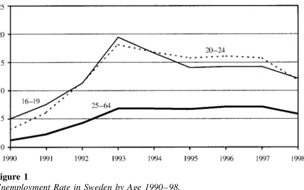
It is a well-known fact in many European countries that youth unem-ployment is more sensitive to uctuations in the business cycle than adult unemploy-ment. Traditionally, this also has been the case in Sweden. The unemployment rates of the youth labor force have also been higher. Thus, the explosive rise in youth unemployment during the crisis of the 1990s is hardly surprising: From a level of around 3 percent in 1990, the unemployment rate for individuals aged 20–24 rose to above 18 percent in 1993, as shown by Figure 1. For the youngest age group, the
Laura Larsson is a researcher at the Institute for Labour Market Policy Evaluation (IFAU), Uppsala, Sweden. She is grateful to Per-Anders Edin, Denis Fouge`re, Bertil Holmlund, Per Johansson, Jochen Kluve, Winfried Koeniger, Michael Lechner, Gerard van den Berg, and two anonymous referees for their helpful comments. Previous versions of this paper were presented at the IZA Summer School in Munich, EALE 1999, the IWH workshop in Halle, and seminars at IFAU and the Department of Eco-nomics in Uppsala. The author claims responsibility for all remaining errors. The data used in this arti-cle can be obtained beginning April 2004 through March 2007 from Laura Larsson, IFAU, P.O. Box 513, S-751 20 Uppsala, Sweden. E-mail: laura.larsson@ifau.uu.se.
[Submitted October 2000; accepted May 2002]
ISSN 022-166XÓ2003 by the Board of Regents of the University of Wisconsin System
Figure 1
Unemployment Rate in Sweden by Age 1990– 98.
Source: Statistics Sweden, Labor Force Surveys.
level of unemployment was even higher until 1994. Adult (aged 25–64) unemploy-ment rose from slightly more than 1 percent to 7 percent. After the peak in 1993, the situation has improved for the young cohorts, whereas adult unemployment re-mained on the same level until 1997.
In response to rising unemployment gures, the Swedish government increased its spending on active labor market policy in order to improve the chances of the unemployed to return to regular employment. In 1992, a new large-scale program called youth practice, targeted at unemployed youth, was introduced. Since partici-pants in active labor market programs are dened either as employed or as being outside the labor force, the immediate effect of such programs is that unemployment falls.1But this is solely a matter of accounting, whereas the longer-term effects re-main largely uncertain. Thus, the evaluation of active labor market programs has become an increasingly important issue.
This paper evaluates the two most comprehensive active labor market programs in Sweden for youth, aged 20–24 years, in the rst half of the 1990s, namelyyouth practiceandlabor market training. The objective is to determine the effects of the programs as compared to the outcome if the individual had continued to search for a job as openly unemployed.2The effects are measured in terms of earnings, employ-ment probability, and the probability of entering studies provided by the regular educational system. The focus is on the direct effects of the programs; no attempt is made to assess the general equilibrium implications.3
1. In principle, participants in training programs (including youth practice) are excluded from the work force, whereas subsidized work programs are dened as employment.
Identication of the average treatment effects is based on the conditional indepen-dence assumption (CIA), according to which participation in the various programs is independent of the post-program outcome, conditional on observable factors in-uencing both the decision to participate and the outcome. Given the CIA, matching on the propensity score using the multiple treatment approach introduced by Imbens (2000) and Lechner (2001) can be applied to obtain unbiased estimates of the average treatment effects on both the treated and the population. Here, a part of the paper is devoted to discussing the plausibility of the CIA in this context. Indirect tests of the CIA, as suggested by Heckman and Hotz (1989), are discussed, and the matching method is compared to some alternative, well-known methods for estimating average treatment effects based on different identifying assumptions.
Previous microeconomic studies of active labor market programs for Swedish youth report varying results. Edin and Holmlund (1991) and Korpi (1994) nd nega-tive effects on post-program employment, but posinega-tive or insignicant effects on the re-employment probability in subsequent unemployment spells. Ackum (1991) and Regne´r (1997) mainly estimate negative program effects on earnings. However, ex-cept for Regne´r (1997), these studies use the same small data set from the 1980s, and apply methods that rely on restrictive parametric assumptions. None of the previ-ous studies evaluates the effects of youth practice.
Consequently, this study contributes to the Swedish and the international literature in several ways. First, it provides a number of new results on the effects of youth programs in Sweden. Second, it applies recently developed methodology to program evaluation. Third, it offers an example of how to make use of data based on compre-hensive Employment Service records.
The paper is organized as follows. The evaluation problem, as well as the identi-cation and estimation of average treatment effects under the conditional indepen-dence assumption is addressed in Section II. The labor market programs and the data are described in Section III. Section IV outlines the econometric analysis based on the propensity score matching approach, while Section V considers the sensitivity of the results. Section VI contains a discussion of alternative identication strategies and ways of (indirectly) testing conditional independence, and, nally, Section VII concludes.
II. Econometric Evaluation Strategies
A. The Evaluation Problem
This study attempts to determine and compare the outcomes of three alternative strategies available to a young unemployed individual: to participate in either youth practice or labor market training, or to continue searching for a job as openly unem-ployed. In other words, the aim is to determine the causal effect of a program com-pared to (1) the no-program state, and (2) the other program. Following Lechner (2001), among others, this multiple evaluation problem may be introduced as fol-lows.
Consider participation in (M11) mutually exclusive treatments, denoted by an assignment indicator TÎ{0, 1, . . . , M}. Let the zero category indicate the no-treatmentalternative. Moreover, denote variables unaffected by treatments, often calledattributes(Holland 1986) orcovariates, byX. The outcomes of the treatments are denoted by {Y0,Y1, . . . ,YM} and, for any participant, only one of the components can be observed in the data. The remainingMoutcomes are called counterfactuals. The number of observations in the population isN, such thatN5åM
m50Nm, where Nmis the number of participants in treatmentm.
The evaluation problem is to dene the effect of treatmentmcompared to treat-mentl, for all combinations ofm,lÎ {0, 1, . . . ,M},m ¹l. More formally, the outcomes of interest in this study are shown in the following equations:
(1) qml
0 5E(Ym2Yl|T5m)5E(Ym|T5m)2E(Yl|T5m), (2) gml
0 5E(Ym2Yl)5EYm2EYl.
qml
0 in Equation 1 denotes the expected average treatment effect of treatment m, relative to treatmentl, for participants in treatmentm(sample sizeNm). In the binary case, wherem51 and l50, this is usually called the ‘treatment-on-the-treated’ effect.gml
0 in Equation 2 is the corresponding expected effect for an individual drawn randomly from the whole population (N).4
The evaluation problem is characterized by missing data: the counterfactual
E(Yl|T
5m) for m ¹l cannot be observed, since it is impossible to observe the same individual in several states at the same time. Thus, the true causal effect of treatmentm relative to treatmentlcan never be identied. However, the average
causal effects dened by Equations 1 and 2 can be identied under the conditional independence assumption; see subsection 2.3.5
B. Matching as an Evaluation Estimator
In experimental studies, participants are randomly assigned to treatment(s) from a large group of eligible applicants. In a binary case, a comparison between the treated and the control group, which consists of the individuals not assigned to the treatment, yields an unbiased estimate of the average treatment effect. Similarly, in a multiple case, an unbiased estimate of the average effect of one treatment compared to another is obtained by comparing the two randomly assigned treatment groups. This is not the case in nonexperimental studies, because the various treatment groups are likely to differ from each other in a nonrandom way. Hence, the objective of a
nonexperi-4. Note that the latter expected effect is symmetric in the sense thatgml
0 5 2glm0, whereas the same is not
valid for the treatment effect on the treated, that isqml
0 ¹2qlm0, as long as participants in treatmentsmand ldiffer in a nonrandom way.
mental evaluation study is to construct a comparison group that is as close as possible to the experimental control group. One method suggested for solving this problem is matching.
Matching methods have been developed and widely used in the statistics and medi-cal literature (Rubin 1977; Rosenbaum and Rubin 1983, 1984, 1985; Rubin and Thomas 1992), but are relatively new to economics and labor market policy evalua-tion. In short, matching involves pairing individuals from various treatment groups who are similar in terms of their observable characteristics. When selection into treatments and the outcome are based exclusively on these observable characteristics, matching yields unbiased estimates of the average treatment effects.
C. Conditional Independence Assumption
The crucial assumption behind matching is that all differences affecting the selection and the outcome between the groups of participants in treatmentmand treatmentl
are captured by (to the evaluator) observable characteristics,X. In the evaluation literature, this assumption is called conditional independence, or unconfoundness. In the multiple case considered in this paper, the conditional independence assump-tion (CIA) is formalized as6
(3) {Y0,Y1, . . . ,YM}IIT|X
5x,"xÎ c,
where II is a symbol for independence andcdenotes the set of covariates for which the average treatment effect is dened. In words, the CIA requires treatmentTto be independent of the entire set of outcomes, givenX. That is, given all the relevant observable characteristics (X), when choosing among the available treatments (in-cluding the no-treatment alternative), an individual does not base her decision on theactualoutcomes of the various treatments.7Individuals can, however, base their decisions on expected outcomes, as long as these are determined byXonly. This implies that individuals expect their outcomes to equal the mean outcomes for people with similar (observed) characteristics. Moreover, in order for the average treatment effect to be identied, the probability of treatmentmmust be strictly between zero and one:
(4) 0,Pm(x)
,1, where Pm(x)
5E[P(T5m|X5x)], "m50, 1, . . . ,M. In the binary case of two treatments, Rosenbaum and Rubin (1983) show that if the CIA is valid forX, it is also valid for a function ofXcalled thebalancing score b(X), such thatXIIT|b(X). The balancing score property holds even for the multiple case:
6. The signicance and consequences of the CIA in the binary case of one treated and one nontreated state have been explored and formalized by Rubin (1977) and Rosenbaum&Rubin (1983). The analysis of the multiple case presented here closely follows the analyses in Lechner (2001) and Imbens (2000). 7. Naturally, for identi cation of a single treatment with xedmandl, it is sufcient to assume pair-wise independenceYlIIT
(5) {Y0,Y1, . . . ,YM}IIT|X
The main advantage of the balancing score property is the decrease in dimension-ality: Instead of conditioning on all the observable covariates, it is sufcient to condi-tion on some funccondi-tion of the covariates. In the binary case of two treatments, the balancing score with the lowest dimension is the propensity scoreP1(x)
5E[P(T5 1|X5x)]. In the case of multiple treatments, a potential and quite intuitive balancing score is theM-dimensional vector of propensity scores [P1(x),P2(x), . . . ,PM(x)]. Lechner (2001) shows, however, that the dimension can be further reduced to two, or even one. This is illustrated in the following section, which addresses identica-tion of the average treatment effects.
D. Identication
Let us begin by considering the identication and estimation of the average treatment effect on the treated,qml
0. The mean outcome of treatmentmfor participants inm, E(Ym|T
5m), is identied and estimated by, for example, the sample mean. Lechner (2001) and Imbens (2000) show that the latter part of Equation 1, the mean outcome of treatmentlfor participants inm,E(Yl|T
5m), can also be identied in sufciently large samples, given conditional independence. To estimate it, they show that instead of theM-dimensional balancing score, the dimension of the condition set can be reduced to [Pm(x),Pl(x)]. Thus,
(6) E(Yl|T
5m)5E[E(Yl|Pm(X),Pl(X),T
5l)|T5m]. Lechner (2001) shows that the dimension can be further reduced: (7) E(Yl|T
5m)5E[E(Yl|Pl|ml(X),T
5l)|T5m],
wherePl|mlis the conditional choice probability of treatmentl, given either treatment morl. Both Equations 6 and 7 are suggested for estimating the average treatment effect on the treated.8
The identication and estimation of the average treatment effect for the whole population, gml
In words, Equation 8 implies that the average treatment effect on the population is identied by a weighted sum of the treatment effects on all subsamples. For a more detailed description of the identication of qml
0 and gml0, see Imbens (2000) and Lechner (2001).
III. The Programs and the Data
Conditional independence cannot be regarded as a plausible assump-tion unless one is acquainted with the instituassump-tional settings —what was the purpose and content of the program? who participated and why? —and has reliable data on all these factors.
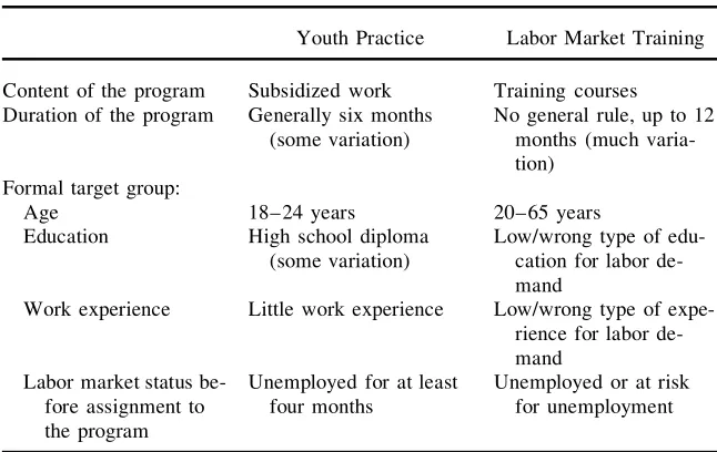
A. Description of the Programs
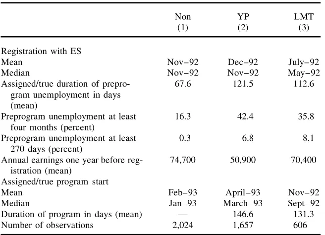
Youth practice (ungdomspraktik) was launched in July 1992, during the most severe period of rising unemployment in Swedish postwar history. By January 1993, the stock of participants aged 20–24 in youth practice reached its peak at 60,000, which corresponds to approximately 10 percent of the population in this age group.9 Simul-taneously, labor market training, the second largest program for that cohort, de-creased from about 25,000 to 15,000 participants. During the period of July 1992– July 1993, participants in these two programs on average accounted for 85 percent of all people in this age group taking part in any program; in the following year, the share was 75 percent.10In October 1995, youth practice was replaced by new programs.
Youth practice consisted of a subsidized work program aimed at providing work-ing experience for the young unemployed with a high school diploma.11Participants were placed in both the private and the public sector, and the program period was generally six months. For individuals aged 20–24, the allowance for participation was SEK 33812per day, of which the employers paid only a very small fraction. In the relatively rare cases where the participant was entitled to unemployment benets, she received an allowance equal to the benet.
According to the program regulations, participation should be preceded by at least four months’ active job search as openly unemployed. In addition, participants should be a supplementary resource for the employer and not displace regular em-ployment, and they should allocate 4–8 hours a week to job-seeking activities at the local employment ofce. In practice, however, participants often worked with tasks that would otherwise have required hiring a regular employee, and allocated very
9. Unemployed individuals aged 18–19 were eligible for youth practice but not for training. Thus, they are excluded from the study in order to fulll the balancing score property,XIIT|b(X).
10. Thus, it seems plausible to focus on the evaluation of these two programs only.
11. Formally, the program was supposed to be a ‘‘mixture of subsidized work and training’ ’ in the sense that it would improve the participants’ human capital. However, implementation studies show that the tasks were often very simple, so that the share of training was more or less negligible (see, for example, Hallstro¨m 1994 and Schro¨der 1995).
Table 1
Differences between Youth Practice and Labor Market Training
Youth Practice Labor Market Training Content of the program Subsidized work Training courses
Duration of the program Generally six months No general rule, up to 12 (some variation) months (much
varia-tion) Formal target group:
Age 18–24 years 20–65 years
Education High school diploma Low/wrong type of edu-(some variation) cation for labor
de-mand
Work experience Little work experience Low/wrong type of expe-rience for labor de-mand
Labor market status be- Unemployed for at least Unemployed or at risk fore assignment to four months for unemployment the program
little time to job seeking.13Moreover, the length of preprogram unemployment varied noticeably from two or three days to several months.
Labor market training, which has existed in various forms for decades and is still in effect, is aimed at improving the skills of the unemployed job seeker in order to match her to labor demand. Thus, it has traditionally been directed at individuals with low education and skills. However, the Swedish high school system seldom prepares fully trained workers, so that individuals with a high school diploma are part of the target group. The program consists of courses of various length and con-tent, both vocational and nonvocational.14The age limit and the size of the allowance have changed over time, but during the period under study, the minimum age limit for participating in the program was 20 years. Moreover, the size of the allowance was the same in labor market training as in youth practice, and, according to the program regulations, participants should continue their job-seeking activities during the program. Table 1 summarizes the differences between the two programs.
Typically, an unemployed individual, in consultation with a placement ofcer at the local employment ofce, decided whether to participate in any of the programs and which program to choose. The reason for wanting to participate varied. Except for individuals who were eligible for unemployment benets (and who thus received the same amount as participants in the programs), participation in either of the pro-grams implied a nancial benet. Moreover, surveys among job seekers and
place-13. For example, participants might assist with some simple administrative tasks in a rm, or take care of children at a daycare center.
ment ofcers indicate that many job seekers believed that participation in a program would improve their chances of nding a job, and many regarded youth practice as a ‘‘real job’’ (see, for example, Hallstro¨m 1994; Schro¨der 1995; Eriksson 1997).
An individual interested in youth practice was usually encouraged by the place-ment ofcer to nd an employer willing to offer placeplace-ment. This was intended to increase the individual’s power of initiative. Consequently, individuals who managed to nd an employer on their own might have had a better chance of participating than those who needed assistance from the local employment ofce. Sometimes, employers took the initiative and offered placement in youth practice if the local employment ofce arranged the nancing.
Rejecting an offer to participate could, in principle, lead to suspension from unem-ployment benets, if the unemployed person was entitled to any. However, in a situation where local employment ofces were deluged with job searchers, those who needed help the most, comprising the least educated and experienced— and not entitled to benets—were most likely to receive an offer, with perhaps one excep-tion. In Sweden, unemployment benets expire after 300 unemployment days unless the individual has qualied for a new 300– day period by working or participating in a labor market program for at least six months.15Therefore, unemployed people close to the benet expiration date may have been more likely to be assigned into a program; see Section IIIA.
To conclude, it is reasonable to assume that the more experienced and better edu-cated the unemployed individual and the shorter her unemployment period, the lower the probability of being offered and assigned to a program. Moreover, having a high school diploma should increase the propensity for youth practice relative to labor market training.
B. Description of the Data
The data used in this study, a random sample of approximately 200,000 individuals, were collected from the databases maintained by the Swedish National Labor Market Board and Statistics Sweden. The former database includes records of all individuals who have been registered with the Employment Service, whereas the latter records the annual earnings of all individuals residing in Sweden. For each individual in this study, registration dates, labor market status, and individual characteristics between August 1991 and March 1997 were combined with information on annual earnings for the years 1985– 95. A more exact description of the variables used in the empirical analysis is given in Tables A1–A3 in the Appendix. Details regarding the outcome variables are given in Section IIIE.
In the Employment Service records, each job seeker is registered under some ‘‘job-seeker category’’ dening her labor market status. Examples of such categories are full-time openly unemployed, part-time openly unemployed, or participant in a labor market program. When signing up with the Employment Service, the unem-ployed persons are asked to ll out a ‘‘search form’’ that contains questions about individual characteristics, such as year of birth, citizenship, formal education, previ-ous labor market experience, and type of job they are looking for. If an individual
wishes to apply for several jobs, she is asked to give each application either a high or a low priority. The job seeker’s county of residence and the code of the local employment ofce she visited are also recorded.
During a period in the Employment Service register, an individual may—and probably will—change categories prior to de-registration. In other words, an individ-ual may have entered the register as openly unemployed, then participate in some labor market program, and again be openly unemployed before de-registration due to, for example, the transition to a regular job. All the relevant dates are provided in the data. The reason for de-registration is also recorded.
The database at Statistics Sweden covers all individuals residing in Sweden at the end of December each year. Information on earnings is based on rms’ reports to the tax authorities. Earnings are measured on a yearly basis, and there is no informa-tion about the number of working hours. As a dependent variable in the empirical analysis of earnings, I used the annual sum of work-related income including the allowance for maternity or sickness leave and other work-related allowances from the social insurance system. Unemployment benets are, of course, not included in this variable. The variation in the dependent variable can thus reect changes in both wage rates and working hours.
C. Is it Plausible to Assume Conditional Independence?
The description of the programs indicates that the level of education, previous work experience, and preprogram unemployment history are important factors in de-termining whether an individual will participate in any program, as well as in which of the programs. These factors are also likely to inuence the future labor market outcome, and thus, in order for conditional independence to be plausible, they should be included in the estimation of the propensities.
The importance of labor market history prior to a program is emphasized in various evaluation studies, starting with Aschenfelter (1978). Examples of more recent stud-ies that all point to pretraining earnings as one of the most essential factors to be controlled for in a labor market program evaluation are Hotz, Imbens, and Mortimer (1998); Dehejia and Wahba (1999); Heckman, Ichimura, Todd, and Smith (1998). Annual earnings for the preceding year, pretraining unemployment periods, level of education, and work experience are all included in the data available for this study.16Moreover, the data provide detailed information on other personal character-istics (see Table A2). Information is missing on whether a job searcher is entitled to unemployment benets that, as discussed above, may provide an incentive to participate in a program. However, there are two arguments that may alleviate this potential shortcoming.
First, entitlement requires work experience which, in turn, implies labor earnings. Thus, by controlling for the latter two, we indirectly control for entitlement. Second, the mean preprogram unemployment periods in the participant samples are far from
300 days, which is the benet exhaustion limit.17Consequently, it is reasonable to assume that the participation decision of these individuals, even if entitled to benets, is not signicantly inuenced by qualication for a new benet period.
A factor often suggested as causing selection bias is ‘‘motivation’’ or some other unobservable personal quality of the job searcher that makes her more or less suc-cessful on the job market, and that also plays a role in the program assignment process.18It may be that the most highly motivated job seekers show the most interest in a program, and are thus most likely to be assigned to it. The opposite is also plausible: Caseworkers may be more eager to help the unemployed persons who are the least motivated. Either way, the estimated program effect will turn out to be biased.
In the Employment Service data, each openly unemployed job seeker is assigned a grade indicative of her readiness to take a job if employment is found. Examples of grades are ‘‘can take a job directly’’ or ‘‘needs guidance.’’ This grading is based on the employment ofcer’s assessment of the job seeker and thus provides a mea-sure of the job seeker’s expected success on the job market.
Finally, the willingness to assign people into programs in general, and into the two programs under study in particular, varied among the local employment ofces. It may be that the willingness to assign into programs is correlated with the ability to match the unemployed people with employers. Thus, variables based on records from the local employment ofces also are included in the estimation of the propensi-ties.
The bottom line is that the available data include much, but not necessarily all, information on factors which affect the selection and the outcome. The crucial ques-tion— that is left to the reader to decide—is whether there issufcientinformation to justify the conditional independence assumption.
Later on, in Section VI, I discuss different ways of indirectly testing the plausibil-ity of the CIA, either through preprogram outcome tests suggested by Heckman and Hotz (1989) or by applying various methods to the same problem and comparing the results. In short, I nd that different methods produce somewhat different esti-mates for the program effects, but the sign of the effects is essentially the same across methods. Moreover, the preprogram outcome tests—as far as it is possible to apply and draw conclusions from them—provide support for the conditional inde-pendence assumption.
D. Sample Construction
From the database, I collected all individuals aged 20 to 24 who registered with the Employment Service during 1992 and 1993 as openly unemployed for the rst time and with the grade ‘‘can take a job directly.’’ This procedure yielded 10,579 individ-uals. From this group, I then collected all individuals who, after having been openly unemployed, directly enrolled in youth practice or labor market training. The nal
17. Table A1 in the Appendix shows that only 7–8 percent of the program participants had been unem-ployed more than 270 days before the start of the program.
group consisted of 1,657 youth practice participants and 606 labor market training participants.19
A potential comparison group consisted of individuals who entered the register as openly unemployed during the same period, and never participated in any of the programs. There were slightly more than 5,000 such individuals. All of them could, in principle, have been used as the group of nonparticipants in the empirical analysis. However, as already pointed out, the length of the unemployment period immediately before starting a program is an important factor in determining whether an individual will participate in any program and to which program she will be assigned. Hence, in order to be able to use this information when estimating of the propensities, I created a hypothetical starting date for nonparticipants. The following procedure is similar to therandom procedure suggested by Lechner (1999).
First, the group of participants (here, participants in practice and training are re-garded as a single group) and the group of nonparticipants were divided into sub-groups by the month of registration with the Employment Service. Then, each of the nonparticipants in a subgroup was randomly assigned an observation of ‘‘length of preprogram unemployment’’ from the distribution of the contemporaneous group of participants. In cases where the nonparticipant’s actual unemployment period was shorter than the assigned preprogram unemployment period, the individual was re-moved from the sample. This procedure deleted approximately 60 percent of the sample and left me with slightly more than 2,000 nonparticipants.20
It should be noted, however, that this group of nonparticipants does not necessarily represent a world without programs; such a construction is possible only in a case where the individuals know that choosing not to participate implies that they will never take part in that particular program. This is not a realistic assumption for Sweden, however, where most programs continue to exist, and the unemployed who have not succeeded in nding a job (or are deregistered from the Employment Ser-vice for some other reason) are offered new possibilities to participate.21Thus, in a strict sense, the 2,000 individuals in the comparison group represent the alternative not to participate but towait, when the rst chance is offered to them. But, they are referred to as nonparticipants because they never participated in any program.
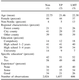
Tables A1–A2 in the Appendix report descriptive statistics of some selected vari-ables for the three groups. There are clear differences in both the program
character-19. By restricting the program period to represent a second ‘‘job seeker category,’’ heterogeneity in the participants’ unemployment history could be reduced. Moreover, choosing therstprogram for every unemployed also appears to be the easiest way of handling multiple program participation. For a discussion of this dynamic program evaluation problem, see among others Gern and Lechner 2002; and Lechner and Miguel 2001. I also removed observations with negative program periods or other curious dates from the complete sample of 10,579 individuals.
20. This group of nonparticipants consists of individuals with, on average, longer unemployment periods than the original group of 5,000 individuals, because the risk of being excluded from the sample due to a ‘‘too late’’ assigned start of the program is higher, the shorter is the individual’ s unemployment period. This is desirable, however, because the aim is to match participants with nonparticipants who were unem-ployed long enough to bepotentialprogram participants.
istics as well as the individual characteristics among participants in various states. As shown in Table A1, the duration of both preprogram unemployment and the program itself are shorter among participants in labor market training as compared to youth practice participants.
Moreover, the sample of labor market training participants consists of individuals who were registered with the Employment Service quite early and thus also started the program earlier than the practice participants. There are also differences in age, citizenship, education, and experience among the three groups.
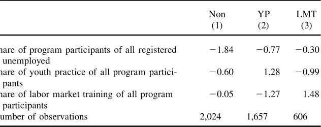
Table A3 lists some selected statistics from the local employment ofces. I assume the probability of being assigned into one of the three states to depend on, among other things, the proportion of all unemployed assigned to any program at the specic local employment ofce, the month before the actual assignment. That proportion may be considered a measure of how readily the ofce assigns individuals to pro-grams. Furthermore, the decision between the two programs is assumed to be depen-dent on the ratio between participants in these programs. Given that these gures also reect local labor market conditions and/or the effectiveness of the ofces in nding jobs, they should be included in the propensity estimations.
As expected, the share of youth practice assignments is above the country average in the sample of youth practice participants. A corresponding pattern holds for train-ing. Somewhat surprisingly, though, the total number of program assignments is below the country average in all three samples. As expected, however, the ratio is lowest in the sample of nonparticipants.
E. What is the Outcome of Interest?
An explicit aim of active labor market policy is to improve the employability of the unemployed people. Hence, a higher probability of future employment and higher earnings are obvious measures of a program’s success. However, especially in the case of youth, a possible track to stable future employment might be regular educa-tion. Thus, in addition to employment probability and earnings, I used the probability of transition from unemployment to studies as a third measure of success.
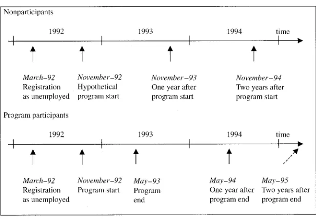
Earnings are measured by a continuous variable, whereas dummy variables were constructed for the other outcome measures. Figure 2 illustrates the way the various outcomes are dened for a hypothetical individual in the sample. This individual signs up with the Employment Service in March 1992. In November 1992, she en-rolls in youth practice for a period of six months. She is dened as ‘‘employed within one year (two years) after program start’’ if she is deregistered from the Employment Service due to regular employment by November 1993 (1994). Analogous denitions are used for regular education.22
Earnings one and two years after the start of a program are measured in a slightly less precise manner because I only had access to an annual sum of earnings with no information on working hours. For an individual who enrolled in a program during the rst half of a calendar year, ‘‘earnings one year after program start’’ comprise
Figure 2
A Registration Period and Its Outcome Measures
the annual sum of earnings for the following calendar year. For individuals who started their program in July–December, I instead use the average of the following two calendar years to avoid counting (zero) earnings during or directly after the start of the program. Thus, for the hypothetical individual in the above example, ‘‘earn-ings one year (two years) after program start’’ are the average of her earn‘‘earn-ings in 1993 and 1994 (1994 and 1995). Nonparticipants’ earnings are similarly dened
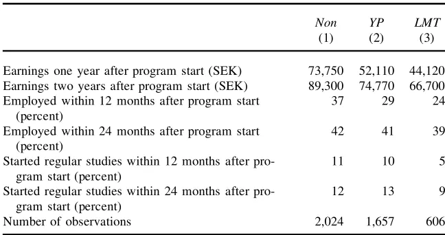
Table 2
Sample Means of the Outcome Measures
Non YP LMT
(1) (2) (3)
Earnings one year after program start (SEK) 73,750 52,110 44,120 Earnings two years after program start (SEK) 89,300 74,770 66,700 Employed within 12 months after program start 37 29 24
(percent)
Employed within 24 months after program start 42 41 39 (percent)
Started regular studies within 12 months after pro- 11 10 5 gram start (percent)
Started regular studies within 24 months after pro- 12 13 9 gram start (percent)
Number of observations 2,024 1,657 606
using the hypothetical start of a program as described in Section IIID.23Table 2 shows that, in the raw data, all average outcome measures except the long-term study effect are highest for nonparticipants and lowest for participants in labor market training.
IV. Empirical Application
A. Estimation of the Propensity
The matching algorithm applied in this study is, in many respects, similar to that in Lechner (2001), and it is outlined in detail in Appendix 2.24The discrete choice model for estimating the propensities is a multinomial logit model with three alternatives: (10) Pr(Ti5l)5
exp(Xihl)
^
Mm50
exp(Xihm) ,
wheremindexes the choice, andithe individual. Xis a vector of covariates. The choice alternatives are no treatment (T50), youth practice (T51), and labor market training (T52) and thus,M52.25To test the assumption of the independence of irrelevant alternatives (IIA) underlying the multinomial logit model, I estimate bino-mial logit models for all three comparisons: (0,1); (0,2); and (1,2). The estimated coefcients of the binomial and multinomial models are similar and, thus, the IIA assumption is considered to be sufciently valid.26
The results in Table A4 in the Appendix show that the statistical signicance of various explanatory variables differs across the two programs. However, the vari-ables for preprogram unemployment history, as well as those from the local employ-ment ofces seem to be highly signicant in general. It is shown in Section V that they play an important role for the results: Excluding them from the propensity esti-mation would signicantly alter the results.
23. I also estimated the treatment effects using earnings for the subsequent calendar year for all participants independent of the starting date of the program. As expected, the results for ‘‘earnings one year after the program start’’ are clearly more negative. For example, the effect of youth practice on participants is 10 percentage points lower than the effect reported in Table 3. The relative effectiveness of the programs, however, is not affected to any large extent by the different denitions of the outcome variable, nor by the effect after two years, which indicates that the earnings effect is stabilized quite rapidly after a program ends. The results can be obtained from the author on request.
24. Heckman, Ichimura, and Todd (1998) suggest other possible estimators. Estimators based on nonpara-metric kernel regressions have somewhat better asymptotic properties, whereas the main advantage of the estimators suggested by Lechner (2001) is their computational simplicity.
25. The specication of the multinomial logit is based on likelihood-ratio tests for omitted variables in a binary framework.
The predictive power of the model is reported in Table A5, and I consider it satisfactory: Approximately 60 percent of the observations are predicted correctly when the highest of the propensities determines the prediction. At least 70 percent of the observations in the subsamples of nonparticipants and youth practice partici-pants are correctly predicted. Outcomes in the smallest subsample of labor market training, though, are merely predicted correctly in 7 percent of the cases.27However, the crucial outcome of interest is the match quality produced by the model, discussed in the next subsection.
A correct estimation of the average treatment effects,qml
0 andgml0, requires common support for the treatment and the comparison group, or 0,Pm(x)
,1 for allm5 0, 1, . . . ,M. In practice, this implies that some of the observations are excluded from the sample, if the propensity distributions do not cover exactly the same interval. In other words, an observation in the subsamplemwith an (estimated) propensity vector equal to {p*1,p*2, . . . ,p*M} was excluded from the sample if any of these propensities was outside the distribution of that specic propensity in any of the other subsamples
l.28Due to this common support requirement, approximately 200 observations were deleted, leaving a sample size of 4,084.
B. Matching
In the binary case of two treatments, the subsample of nonparticipants generally consists of a large number of observations, and it is thus plausible to use each com-parison unit only once. This is not meaningful in the multiple case, since pair-wise comparisons were made across all subsamples, and for some comparisons, the poten-tial comparison group is much smaller than the treatment group. Thus, matching was done with replacement, whereby each comparison unit was allowed to be used more than once, given that it was the nearest match for several treated units. The covariance matrix for the estimates of average effects, proposed in Lechner (2001), considers the risk of ‘‘over-using’’ some of the comparison units: The more times each comparison is used, the larger is the standard error of the estimated average effect.
A detailed description of the matching algorithm is outlined in Appendix 2. The pair-wise matching procedure was carried through six times altogether. Each individ-ual in the treated subsamplemwas matched with a comparison in subsamplel. The criteria for nding the nearest possible match was to minimize the Mahalanobis distance of [Pm(X),Pl(X)] between the two units.
Furthermore, covariates in the matched samples ought to be balanced according to the conditionXIIT|b(X), referred to as the balance of the covariates. Following Lechner (2001), the match quality is judged by the mean absolute standardized biases of the covariates. The results show that the covariates are sufciently balanced by the reported model specication.
27. The distributions of the predicted propensities also should be considered. In a broad outline, a good model produces large differences in the mean of predicted propensities across the various groups. This is the case for propensities to participate in youth practice and to not participate in any program, whereas the distributions of propensities to participate in labor market training look very similar. Once again, this may be a result of the small size of this subsample compared to the other subsamples.
C. Results
Aggregating the pair-wise differences over the common support yields an estimate of the average treatment effects on the treated,qml
0. Average treatment effects on the population, gml
0, are obtained by taking weighted sums of the treatment effects on the treated.29The exact expressions forqml
0 andgml0 are found in Lechner (2001).
1. Average Treatment Effect on the Treated
Table 3 reports the effects of the six different treatments on the treated effects. Each estimated effect is reported in both absolute and relative terms. By presenting the absolute size of the effects, it is possible to compare the magnitude of the effects between the treated and the nontreated. The relative effects indicate the extent of the magnitude of the effect and help to explain how the results are changed due to the sensitivity analysis in Section V.
First, let us compare the programs to the state of no participation shown in the rst four columns. Columns 1 and 3 report the program effects on program participants, as compared to nonparticipation, whereas the potential effects on those who did not participate in any program are shown in Columns 2 and 4. The last two columns report the effects of youth practice as compared to training, rst on participants in practice and then in training.
In general, there is little heterogeneity between the groups; for example, the effects of youth practice compared to nonparticipation are roughly the same for participants and nonparticipants. The short-term effects on both earnings and employment are signicantly negative for both programs and all groups throughout.30However, after two years from the start of a program, they are more positive and the only signi-cantly negative results are found for the effects of labor market training on earnings. Youth practice does not seem to have any effect on the probability of entering educa-tion, whereas participation in labor market training would have signicantly de-creased the study probability of nonparticipants, as shown in Column 4.
A comparison of the two programs indicates that practice was better than training for those actually participating in it in terms of all outcome measures. All effects reported in Column 5 are statistically signicant and positive except for the long-term employment effect. For the group of participants in labor market training, the difference between the programs seems to be less signicant, although in the same direction, as for youth practice participants.
29. The weights for calculating the average population effect of treatmentmcompared to treatmentlare based on the number of times each unit is used in all comparisons, that is, not only the comparisons between treatmentsmandl. Consequently, the average population effect may differ quite considerably from the average of the treatment effects on the treated, (qml
0 1(2qlm0))/2.
T
h
e
Journal
of
H
um
a
n
R
es
ourc
es
Table 3
Results for the Mean Treatment Effect on the Treated:qml
0 5E(Ym|T5m)2E(Yl|T5m), Expressed in Absolute Terms
YP–Non Non–YP LMT–Non Non–LMT YP–LMT LMT–YP
(1) (2) (3) (4) (5) (6)
Earnings one year after program start (SEK) 214,565 16,380 223,440 27,100 15,560 26,690
(23.82) (4.03) (25.22) (7.16) (3.92) (21.50)
222% 29% 235% 59% 42% 213%
Earnings two years after program start (SEK) 23,330 5,060 214,080 14,450 11,480 22,170
(20.50) (0.76) (22.33) (2.22) (1.45) (20.34)
24% 6% 217% 20% 18% 23%
Employment within 12 months after program 20.07 0.10 20.10 0.11 0.06 20.01
start (percentage points) (22.46) (3.25) (23.30) (3.77) (2.03) (20.16)
218% 37% 230% 41% 27% 22%
Employment within 24 months after program 0.02 0.03 20.01 20.02 0.03 0.00
start (percentage points) (0.82) (1.00) (20.31) (20.64) (0.71) (20.05)
6% 8% 23% 25% 6% 0%
Studies within 12 months after program start 20.01 0.00 20.03 0.06 0.06 20.04
(percentage points) (20.42) (0.05) (21.69) (3.77) (3.20) (22.00)
27% 1% 233% 102% 127% 242%
Studies within 24 months after program start 0.01 20.00 0 0.05 0.04 20.02
(percentage points) (0.64) (0.21) (0) (2.40) (2.06) (0.96)
10% 24% 0% 62% 51% 220%
Number of observations* 1,592–711 1,912–722 580–439 1,852–459 1,592–425 580–388
Notes:Bold typeindicates statistical signicance at the 5 percent level.t-values in parentheses,relative effects in italics. For a description of the dependent variables,
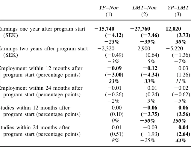
Table 4
Results for the Average Treatment Effect on the Population: gml
0 5E(Ym2Yl)5 EYm
2EYl, Expressed in Absolute Terms
YP–Non LMT–Non YP–LMT
(1) (2) (3)
Earnings one year after program start 215,740 227,760 12,020
(SEK) (24.12) (27.46) (3.73)
223% 239% 30%
Earnings two years after program start 22,320 2,900 25,220
(SEK) (20.49) (0.64) (21.36)
23% 5% 27%
Employment within 12 months after 20.09 20.12 0.03
program start (percentage points) (23.00) (24.34) (1.26)
223% 233% 11%
Employment within 24 months after 20.01 0.01 20.02 program start (percentage points) (20.26) (0.24) (20.62)
22% 3% 25%
Studies within 12 months after 0.00 20.06 0.06
program start (percentage points) (0.10) (23.75) (3.56)
0% 250% 150%
Studies within 24 months after 0.01 20.03 0.04
program start (percentage points) (0.51) (21.93) (2.64)
8% 225% 44%
See notes to Table 3.
2. Average Treatment Effect on the Population
Table 4 reports the estimated average treatment effects on the population. These results conrm the impression given by Table 3: In the short run, both programs result in lower earnings, as well as a lower probability of employment, compared to the outcome without any program. Similar to the treatment-on-the-treated results, the negative effects more or less disappear in the course of time. Youth practice has no effect on the probability of studies, while the effect of labor market training is signicantly negative.
All in all, youth practice seems to have been ‘‘less harmful’’ than labor market training, except for the effect on employment probability, where the difference is statistically insignicant.31
V. Heterogeneity and Sensitivity Analysis
Let us now examine the robustness of the results reported in Section IV. First, the sensitivity of the results to the availability of the covariates is explored.
Second, I examine heterogeneity among various types of individuals, and between various types of labor market training. Third, the denition of the outcome variables is changed in order to examine whether the negative program effects could be a result of declining search activity during participation in a program.
A. Availability of the Covariates
Preprogram earnings and unemployment, local employment ofce variables, and ed-ucation and experience were excluded one by one from the propensity estimation in order to check the sensitivity of the results to the availability of these suggested key covariates. As an example, Table 5 shows the changes in the short-term effects of youth practice on participants.
The results are indeed sensitive to a reduction in information. The initially strong negative earnings and employment effects of youth practice as compared to nonpar-ticipation become less negative when any of the covariates are excluded. Note, how-ever, that the unadjusted differences are more negative than the initial estimates obtained by matching on all covariates. Given that our main model is correctly speci-ed, this suggests that excluding some of the key covariates may sometimes be worse than excluding all of them.
The results further indicate that the importance of a covariate depends on the comparison group. Preprogram unemployment is an example: If it is excluded, the employment and earnings effects of youth practice become less negative when com-pared to nonparticipation, but less positive when comcom-pared to training. The covari-ates also play a different role for different outcome variables. For instance, control-ling for education and experience seems to be important when examining the employment effect, but less so for the earnings effect.
Information on the relative program magnitude at the local employment ofce is always essential when measuring the effect of youth practice. Excluding preprogram unemployment also has an impact on most of the estimates. Moreover, these two variables are important for the estimated effect of labor market training on partici-pants.32
B. Heterogeneity among Individuals
I have examined the variation in the estimated effects (i) between sexes, (ii) among the cohorts of program participants, and (iii) among individuals with various propen-sities to participate in the programs. In short, there is some heterogeneity in all re-spects.
The programs generally seem to have been slightly better for women than for men. The earnings effects are more or less the same for both sexes, whereas the effects on both study and employment probability differ signicantly. This holds for the effects on the treated as well as for population effects. Both programs, but labor market training in particular, have more negative short-term effects on employment for men than for women. Youth practice seems to be superior to, or at least as good as, labor market training for both sexes in all respects.
L
ars
son
911
Sensitivity to the Availability of Covariates; Average Effects of Youth Practice on its Participants
(i) (ii) (iii) (iv) (v) (vi)
Youth practice—nonparticipation
Earnings one year after program 214,565 210,900 28,780 29,000 213,390 221,640
start (SEK) (23.82) (23.04) (23.81) (23.29) (24.99) (10.0)
Employment within 12 months after 20.07 20.04 20.06 20.03 20.02 20.08
program start (percentage points) (22.46) (21.45) (22.74) (21.02) (20.57) (25.16)
Studies within 12 months after 20.01 20.02 20.02 20.04 20.03 20.01
program start (percentage points) (20.42) (21.30) (21.53) (22.29) (21.59) (20.97)
Youth practice—labor market training
Earnings one year after program start 15,560 13,950 8,530 11,980 15,270 8,000
(SEK) (3.92) (3.37) (2.72) (3.68) (4.39) (2.85)
Employment within 12 months after 0.06 0.07 0.04 0.04 0.06 0,05
program start (percentage points) (2.03) (2.30) (1.48) (1.41) (1.85) (2.41)
Studies within 12 months after 0.06 0.05 0.04 0.02 0.06 0.05
program start (percentage points) (3.20) (2.74) (2.08) (1.32) (3.66) (4.20)
Notes:Bold typeindicates statistical signicance at the 5 percent level.t-values in parentheses. (i) All variables included (main model); (ii) preprogram earnings
The state of the business cycle also has an impact. As shown in Table A1 in the Appendix, the dates for the start of a program (or the hypothetical start of a program) vary considerably among the individuals in the three subsamples. In the analysis in Section IV, I did not consider time variation— that is, the fact that ‘‘one year after the start of a program’’ may imply early 1993 for one individual and early 1995 for another. If labor demand or study opportunities vary over the period, the results may be inuenced by the systematic difference in registration dates among the samples.
Besides correcting for a potential bias, an analysis in which participant groups are divided into subgroups by the year of the start of a program may also reveal heterogeneity in the treatment effects among various cohorts of participants. In fact, there turns out to be a considerable amount of variation between the subgroups. The earnings and employment effects of the programs are the least favorable for those who enrolled in a program in 1992, then gradually improve for the latter cohorts of 1993 and 1994. Regarding the study effects, labor market training seems to have a clearly negative effect on the cohorts of 1992 and 1993. For the latest cohort, the employment and study effects of both programs compared to nonparticipation are estimated to be positive, though mainly statistically insignicant.
Heterogeneity was also examined with respect to the propensity of a treatment. A positive correlation between the propensity of a treatment and the treatment effect would indicate that the criteria for assignment are correct. Consequently, a negative correlation, or no correlation at all, implies that the selection rules are not optimal. Plotting the differences in earnings and study probability for each matched pair against the propensity of the treatment indeed reveals a great deal of variation, but no correlation. The effect of labor market training on employment as compared to nonparticipation seems to be slightly more positive, the higher is the propensity of labor market training. In general, however, the average effects of the programs com-pared to nonparticipation and to each other appear to be approximately the same for individuals likely and not likely to be selected into a program, respectively. This, in turn, may imply a nonoptimal selection criteria.
C. Heterogeneity between Various Types of Labor Market Training
Labor market training is a relatively heterogeneous program consisting of courses of various content and length. In a broad outline, the courses are divided into voca-tional and nonvocavoca-tional categories that are often preparatory in the sense that partic-ipants already have ex ante plans to participate in further programs. An example of such courses is Swedish for immigrants. Consequently, participants in these courses are not expected to de-register from the Employment Service as quickly as partici-pants in vocational courses or other programs. The effects of nonvocational courses may thus be less advantageous than those of vocational courses.
Approximately 34 percent of the labor market training participants took a non-vocational course.33To examine whether the effects differ between the two types of training, I applied an analysis where vocational and nonvocational courses were
Figure 3
Outcome Measures When a Program Period is Excluded
treated as separate programs. In short, the results show that the type of training has a relatively small effect. The estimated earnings and employment effects of vocational training are only marginally higher (less negative) than those of nonvocational train-ing. Hence, the strongly negative average effects of labor market training remain robust, even when the various types of training are considered.
D. Denition of the Outcome Variables
The analysis in Section IV is based on the assumption that individuals who partici-pated in the programs continued their job search during the program, as required by the program regulations. Thus, the program period is included in the outcome mea-sures of the participants. However, in practice, search activity may diminish consid-erably during participation in a program. (For evidence, see Ackum Agell 1996; or Edin and Holmlund 1991.) Thus, it might be argued that the program period should be excluded when dening the outcome variables, as illustrated in Figure 3.34
As before, the time span ‘‘within one or two years after’’ begins with the hypothet-ical start of a program for nonparticipants, while for program participants, it instead beginsat the end of a program. In this analysis, earnings after the start of a program are dened as follows. For all program participants with a programend, and for all
nonparticipants with a hypothetical programstart during, say, 1992, earnings one year after theend/startof the program are the annual sum of earnings for the calendar year 1993. Consequently, more positive effects of the programs as compared to the state of no participation would be expected. Moreover, since the average participa-tion period in labor market training is shorter than the average period in youth prac-tice, more positive average effects of practice as compared to training would also be expected.
The results are more or less as anticipated: The earnings and employment effects of both programs are diminished, whereas the study effects are more or less unchanged compared to the effects in Section IV. The effects of youth practice on participants are, in fact, estimated to be slightly positive, though statistically insignicant. Labor market training seems to have negative effects even when the program period is excluded, however. When estimated for the whole population, all three short-run effects are statistically signicant and negative. All in all, it seems that the negative effects of youth practice presented in Section IV may be explained by declining search activity among participants during the program, whereas further explanations are needed to account for the deleterious effects of labor market training.
VI. Discussion on Identication
The fundamental problem of an evaluator is to choose the right esti-mator. The decision should be based on available data and the design of the pro-gram(s), but, in the end, it will always be subjective. As Heckman, LaLonde, and Smith (1999) formulated it, ‘‘there is no magic bullet.’’
In this study, I have based the analysis on the conditional independence assump-tion, according to which the data provide information on all factors affecting selec-tion as well as the outcome. This is a strong assumpselec-tion which, as is always the case with identifying assumptions, cannot be tested directly. However, an indirect way of testing its plausibility, suggested by among others Heckman and Hotz (1989), is to apply the matching estimator to the outcome variables prior to the program period. According to such a test, an insignicant difference in the preprogram out-comes between two groups provides support for conditional independence.
However, as pointed out earlier, all available information on preprogram labor market history should be included in estimation of the propensities. Once this is done, application of a preprogram outcome test is not meaningful, since the matching procedure (applied correctly) implies that the preprogram outcome variables are bal-anced across the samples. That is also the case in this study. Preprogram earnings are included in the estimation of the propensities, and the results for balance of the covariates show that the differences in mean preprogram earnings are negligible among the three samples.35
Another idea for testing the plausibility of the identifying assumption, or at least the robustness of the results, could be to apply various estimators to the same problem to see whether the results differ. It is not obvious how the results of such comparisons should be interpreted, however. Let us say that all methods produce similar estimates for the program effect. What, then, does this say about the validity of the identifying assumptions underlying the various estimators? It might imply that there is no selec-tion at all, a viewpoint supported by, for example, Heckman, LaLonde, and Smith (1999). If so, it would nevertheless convince the evaluator that the estimated program effect is the true one.
Another, perhaps more pessimistic way of interpreting such results is to argue that they only imply that some or all identifying assumptions are invalid without pointing out which ones. According to this view, different estimatorsshouldproduce various results since they are based on various identifying assumptions, and some-thing is wrong— but we do not know what—if they produce the same results.
Bearing these alternative interpretations in mind, I compared the results obtained by matching with some alternative, well-established estimators.36The rst approach involves the standard OLS regression for the continuous dependent variable, and a probit model for the discrete dependent variables. As in the matching approach, identication of the average treatment effects in these models requires conditional independence. Moreover, the estimators are based on further parametric restrictions. The results are reported in Table A6 in the Appendix. The set of covariates in-cluded in the OLS and the probit estimations are the same as those used to estimate the propensity scores. A comparison of Table A6 with Table 3 shows that, in this specic case, OLS and probit on the one hand, and matching on the other produce fairly similar estimates of the average treatment effects on the population. But this is not very surprising since identication is based on the same assumption.
One substantial difference compared to the results obtained by matching, however, is an improvement in the employment effects of youth practice. Table A6 reports a practically zero short-term effect and a signicantly positive effect in the long run, whereas the effects obtained from the matching framework are clearly more negative. Consequently, the difference between the employment effects of practice and train-ing is more obvious in Table A6. Moreover, the long-term earntrain-ings effect of labor market training is estimated to be signicantly negative by OLS, whereas matching obtains a zero effect. These differences are presumably explained by the parametric restrictions underlying the OLS and probit estimations. Matching allows for hetero-geneity in the treatment effects in a more exible way.
A second approach applied to the continuous dependent variable—earnings— is a multinomial generalization of the classical Heckman two-stage model presented by Lee (1983) and called a polychotomous selectivity model. The Lee model is similar to other selectivity models in that it is designed to adjust for both observed and unobserved selection bias. Thus, it does not require the conditional independence assumption to be valid. However, it rests on other strong assumptions, among them linearity in the outcome variable and joint normality in the error terms.
The results are shown in Table A7. The multinomial logit model underlying the inverse Mill’s ratios is exactly the same as the one used to estimate the propensity
scores. The local employment ofce variables are now only assumed to affect the selection into programs but not earnings and are thus excluded from the earnings equation.
The results show fewer negative effects of the programs than matching. The differ-ence between the effects of practice and training is also diminished. The long-term effect of labor market training is estimated to be less favorable than in the short run. Drawing conclusions about the existence of unobserved heterogeneity is not straightforward, however, because the standard errors for the parameter estimates for selection adjustment terms are very large. The precision of the estimates of the treatment effects is also low. In sum, the results seem to suggest that there may be some unobserved heterogeneity between the samples that implies a (moderate) nega-tive bias in the estimated program effects presented in previous sections of this paper, but the evidence is not unequivocal.
VII. Conclusions
The purpose of this study has been to evaluate labor market programs for youth in Sweden using three measures of effectiveness: post-program annual earnings, employment probability, and probability of entering regular education. More precisely, the programs evaluated are youth practice and labor market training. The age group examined is 20–24.
Identication of the average treatment effects is based on theconditional indepen-dence assumption(CIA), whereby participation in the various treatments, including the no-treatment state, is independent of the post-program outcomes conditional on observable exogenous factors. The results from the main analysis suggest that both youth practice and labor market training have negative short-term effects on earnings and employment, where ‘‘short-term’’ refers to one year after the start of a program. Two years after the start of a program, however, the effects are no longer as obvious; most estimates for employment and earnings are statistically insignicant at the 5 percent level. As regards the third measure of effectiveness, the probability of regular education, the results show no signicant effects of youth practice, whereas labor market training may have had a negative effect, at least in the short run. Finally, a comparison of the two programs suggests that practice was better—or ‘‘less harm-ful’’—than training.
How robust are these results? Beginning with the question of identication, neither the preprogram outcome tests nor the comparison with results from other methods seem to give any reason to seriously doubt the plausibility of the CIA in this context. The traditional two-stage selectivity model does indeed yield somewhat different results for both programs than matching, at least in the short run, but the point esti-mates are nevertheless negative. Moreover, drawing conclusions from such method-ological comparisons is not straightforward. Because no direct test for the fundamen-tal identifying assumptions is available, it is ultimately up to the reader to judge the results by weighing in the institutional setting and the available data.