Seasonal and Inter-annual Variability of Sea Surface Temperature and Sea Surface Wind in the Eastern Part of Indonesian Sea: Ten Years Analysis of Satellite Remote Sensing Data.

(1)

(2)

(3)

(4)

(5)

(6)

(7)

(8)

(9)

(10)

(11)

Seasonal and Inter-annual Variability of Sea Surface Temperature and

Sea Surface Wind in the Eastern Part of Indonesian Sea: Ten Years

Analysis of Satellite Remote Sensing Data

I Dewa Nyoman Nurweda Putra*

a,b

and Tasuku Tanaka

a

Graduate School of Science and Engineering, University of Yamaguchi, 755-8611

Yamaguchi Ken, Ube Shi Tokiwadai 2-16-1, Japan;

b

University of Udayana, Bali, Indonesia 80234

ABSTRACT

The overall objective of this study is to gain an improved understanding of the sea surface temperature (SST), sea surface wind speed (WS) and sea surface wind direction (WD) variability in the Eastern part of Indonesian Sea in response to the seasonal and inter-annual variations. The statistical properties and monthly average data for the 10-year period from December 1999-November 2009 in the Eastern part of Indonesian Sea are investigated by integrated use of TRMM Microwave Imager (TMI) of the Tropical Rainfall Measuring Mission (TRMM) and SeaWinds on the Quik Scatterometer (QuikSCAT) satellite remote sensing data. The time series shows a high variability (unstable areas) of SST and WS in the southern equatorial (120o-135oE and 3oS-18oS) in contrast with the stable SST condition around equatorial and other regions. This condition related to the effect of the Indonesian throughflow (ITF) and the prevailing winds in the Indonesian inland seas, which is WD varies seasonally. North-south (zonal) change of SST and WS are observed. These overall analyses confirm several characteristics of the Eastern part of Indonesian Sea.

Keywords: TMI, QuikSCAT, SST, WS, Eastern-Indonesian Sea.

1. INTRODUCTION

The monitoring of large scale patterns of sea surface temperature (SST), sea surface wind speed (WS) and sea surface wind direction (WD) has become possible through the rapid advancement of satellite remote-sensing techniques over the last few decades. The TRMM Microwave Imager (TMI) of the Tropical Rainfall Measuring Mission (TRMM) and SeaWinds on the Quik Scatterometer (QuikSCAT) satellites are kind of such advances, providing more than 10 years (December 1997 to the present time) observations data distributed over global ocean at a pixel resolution of 0.25 deg (~25 km)8. The QuickSCAT, however, continued to operate for a decade and stopped working circa 23 November 2009 due to the failure of the spin mechanism of the anntena1.

The Indonesian Sea, a semi-closed marginal sea, is located at the confluence of the Pacific Ocean and the Indian Ocean between Asia and Australia continent (20S–20N 90–142E; Figure 1). The water is generally shallow (<100 m) throughout the western area of the sea, including the Java Sea and Bali Sea. In contrast, the abyssal Indonesian Sea basin in the southeast reaches depths until 5000 m. The Indonesia Sea is isolated from the western Tropical Paciﬁc Ocean and the eastern Tropical Indian Ocean by a chain of islands and becomes one of the most interesting areas of the world ocean. It provides a unique pathway, the Indonesian throughflow (ITF), for the Western Tropical Pacific water into the Southeastern Tropical Indian Ocean through the Indonesian Seas. On the global scale, the ITF is an important pathway for the transfer of climate signals and their anomalies around the world’s oceans10 with the primarily channels through Makassar Strait, Lombok Strait, Lifamatola Strait, Ombai Strait and Timor passage3.

The present study investigates the inter-annual and seasonal variability of the SST and WS induced by the meandering ITF, El Nino-Southern Oscillation (ENSO) and Indian Ocean Dipole (IOD) phenomena’s over five dominant areas in the Eastern part of Indonesian Sea. An advantage of 10-year period of microwave measurements on the TMI and QuikSCAT satellites were used to reveal and compare their variability. The Empirical Orthogonal Function (EOF) analysis of the interannual variability of local SST over five areas is also reported. Finally, the result of this study is expected to provide relevant information on the features of SST, WS and WD in those areas, and a better understanding of the long-term characteristics of the Eastern part of Indonesian Sea.

Remote Sensing of the Marine Environment II, edited by Robert J. Frouin, Naoto Ebuchi, Delu Pan, Toshiro Saino, Proc. of SPIE Vol. 8525, 85250B © 2012 SPIE · CCC code: 0277-786/12/$18 · doi: 10.1117/12.977398

Proc. of SPIE Vol. 8525 85250B-1

(12)

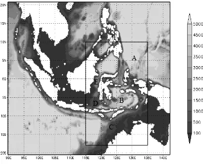
Figure 1. The bottom topography map (scale in meter) of the Indonesian Sea derived from ETOPO 2 minutes9. Axes indicate longitude 90o - 142o E and latitude 20o S - 20o N. Areas with deep water are shaded in light gray, areas with shallow water are shaded in dark gray and areas with no available data are in white.

2. METHODOLOGY

2.1 Study Area

The whole study area is located in the eastern part of Indonesian Seas, between 115o - 135o E and 18o S - 10o N (The rectangular region on Figure 1). This region is divided into five local areas, which is strongly affected by ITF. The five areas study are: area A cover the Equatorial region, between 120o - 135o E and 2o S - 10o N; area B cover the Banda Sea region, between 120o - 135o E and 10o S - 4o S; area C cover the Timor Sea region, between 120o - 135o E and 18o S - 12o S; area D cover the Bali and Flores Sea region, between 115o - 120o E and 7o S - 4o S; area E cover the Makassar Strait region, between 115o - 120o E and 3o S - 2o N.

2.2 Satellite Data Processing

A number of 120 monthly SST and WS for all grid points in the five areas were analyzed in this research. To determine the characteristics of the eastern part of Indonesian seas within the 10 years period from December 1999 through November 2009, the latitudinal averages of seasonal and inter-annual variability of indices for all grid points were calculated from the baseline data.

A

B

C

D

E

(13)

The Empirical Orthogonal Functions (EOF) method was then used to reveal the inter-annual cycle of SST in relation with ENSO and IOD for the five defined areas. As described by Hannachi et al., EOF analysis is a useful technique which decomposes a space-time field into spatial pattern and associated time indices4. The first few modes of the decomposed functions with higher variance may generally have physical significance, while the other functions with small percentage of variance are more difficult to interpret due to the orthogonality constraint6. Usually, most of the possible dynamical mechanisms may be linked to the first few orthogonal functions. This advance technique has found wide application in the various climate data analysis2.

3. DATA

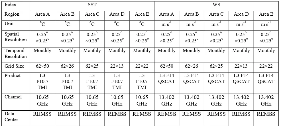
The SST and WS level 3 products of TMI and QuikSCAT data for a 10 years period (December 1999 – November 2009) were used in this study. The temporal resolution of the data is 1 month and the spatial resolution is 0.25o ×0.25o. The data are available to the public at the Remote Sensing Systems (REMSS) for TRMM-TMI and QuikSCAT data (ftp://ftp.remss.com). Since the TMI and QuikSCAT data cover the global area, we need to further extract the data for our study domain, i.e. the five areas A, B, C, D and E that represent the eastern part of Indonesian Seas. The five areas in the study domain are shown on Figure 1 and the specifications of the baseline data are listed in table 1.

Table 1. The specifications of the baseline data.

Index SST WS

Monthly Monthly Monthly Monthly Monthly Monthly Monthly Monthly Monthly Monthly

Grid Size 62×50 62×26 62×25 22×13 22×22 62×50 62×26 62×25 22×13 22×22

Product L3

REMSS REMSS REMSS REMSS REMSS REMSS REMSS REMSS REMSS REMSS

4. RESULTS

4.1 Seasonal Variability in Selected Regions

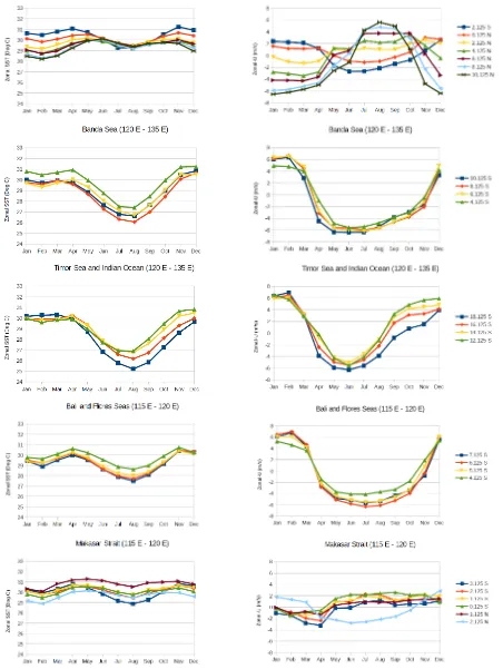
The latitudinal time series of SST and U-WS (U-component (east-west direction) of WS) clearly identify the dominance of the 10 year seasonal signal in each area. Large variability of SST is noticed in the area B and C, with minimum SST occurring during the southeast monsoon (May and September) and maximum SST during Northwest monsoon (November and March). Figure 2 shows the latitudinal SST and U-WS. It is shown that the lowest SST ranging from 25

o

C to 27 oC occurred in the area B and C; the other areas never reach this lowest SST, although the WD (U-WS) changes seasonally. The highest SST occurred in the all area ranging from 30 oC to 31 oC. It is interesting to note that the region of primarily ITF inflow3, the area A and E shows minimum variability with stable warm SST through the year. In the area D also show conspicuously low variability, in association with the stable warm SST supplied from the area E (ITF pathway).

(14)

Figure 2. Seasonal variability and latitudinal averages of monthly SST (left side) and U-WS (right side).

(15)

Figure 3. Inter-annual variability and latitudinal averages of monthly SST (left side) and U-WS (right side).

(16)

4.2 Inter-annual Variability in Selected Regions

The magnitude of inter-annual variability of SST and U-WS on each area from December 1999 to November 2009 is obtained and presented in Figure 3. Among the above areas, the magnitude showed that the temporal variability was mostly constant at a frequency of 12 months, particularly in area B and C. This condition reveals that the year-to-year variability is relatively small compared with seasonal variations. It is also clearly shown that the area B and C have a large peak-to-peak variability within 10 years, in association with the prevailing winds varies seasonally in these areas. The small peak-to-peak variability in the other areas (A, D and E) is strongly correlated with the ITF pathway which supplies a stable warm SST through the year.

4.3 Temporal Variance of EOF Analysis

The Pacific and Indian Oceans, interestingly, are home to the most important phenomena, ENSO and IOD. It is challenging to analyze the influence of the non-seasonal mode of Pacific and Indian ocean-atmosphere variability on each area of our research. On the other hand, according to the small year-to-year variability found in this research, an EOF analysis that simultaneously extracts the recurrent spatiotemporal patterns of natural variability need to be applied in order to recognize such kind of non-seasonal mode. As shown later, the principal component (PC) of EOF analysis can effectively characterize the variability evolution of time series data on each area, in comparison with the Oceanic Nino Index (ONI)7 and Dipole Mode Index (DMI)5.

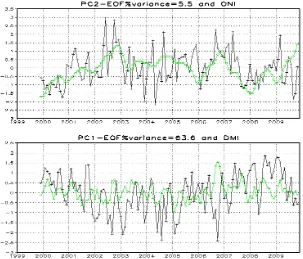
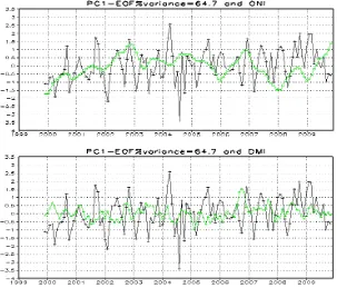
Figure 4. Principal components of EOF-SST anomaly on area A. The upper figure indicates the comparison with ENSO mode and the lower figure indicates the comparison with IOD mode. PC is plotted with cross mark, ONI is plotted with circle mark and DMI is plotted with triangle mark.

In general, the leading PC mode can recognize the temporal variation of ENSO and IOD events within 10 years. The PCs (PC1 and PC2) of areas A, B, C, D and E are plotted in Figures 4, 5, 6, 7 and 8 respectively. These figures confirmed the features of an El Nino event during the period of 2002-2003; 2004-2005; 2006-2007 and La Nina event during the period of 2000-2001; 2006-2007; 2008-2009. PC2 represent the ENSO event in area A and B while PC1 represent this event in the other areas. This indicated the ENSO event account for very small of the data variance (mode 2) in area A and B. The strong positive IOD event during the period of 2006-2007 also can be detected by PC in the five areas. PC1 represent the IOD event in all areas, except for area C.

(17)

Figure 5. Principal components of EOF-SST anomaly on area B. The upper figure indicates the comparison with ENSO mode and the lower figure indicates the comparison with IOD mode. PC is plotted with cross mark, ONI is plotted with circle mark and DMI is plotted with triangle mark.

Figure 6. Principal components of EOF-SST anomaly on area C. The upper figure indicates the comparison with ENSO mode and the lower figure indicates the comparison with IOD mode. PC is plotted with cross mark, ONI is plotted with circle mark and DMI is plotted with triangle mark.

(18)

Figure 7. Principal components of EOF-SST anomaly on area D. The upper figure indicates the comparison with ENSO mode and the lower figure indicates the comparison with IOD mode. PC is plotted with cross mark, ONI is plotted with circle mark and DMI is plotted with triangle mark.

Figure 8. Principal components of EOF-SST anomaly on area E. The upper figure indicates the comparison with ENSO mode and the lower figure indicates the comparison with IOD mode. PC is plotted with cross mark, ONI is plotted with circle mark and DMI is plotted with triangle mark.

(19)

5. CONCLUSIONS

Ten years satellite imagery are analyzed and used to evaluate seasonal and inter-annual variations of SST, WS and WD in the Eastern part of Indonesian Sea. The latitudinal time series clearly identify the dominance of the seasonal signal in the area B and C. A large peak-to-peak variability within 10 years is also clearly shown on the area B and C. These confirm the unstable area in both locations. The PCs of EOF analysis describes non-seasonal mode of Pacific and Indian ocean-atmosphere variability. It is interesting to note that the ENSO and IOD events can be detected by PC1 and PC2, which indicates a great influence of these events in the five areas of study.

REFERENCES

[1] Alan, B., "QuickScat Mission Status Report," <http://winds.jpl.nasa.gov/publications/quikscatStatus.cfm> (20 April 2011).

[2] Antonio, N., Valeria, S., [A Guide to Empirical Orthogonal Functions for Climate Data Analysis], Springer, Dordrecht Heidelberg London New York, 39-64 (2010).

[3] Gordon, A., Sprintall, J., Van Aken, H.M., Susanto, D., Wijffels, S., Molcard, R., Ffield, A., Pranowo, W., Wirasantosa, S., "The Indonesian throughflow during 2004-2006 as observed by the INSTANT program," Dyn. Atmos. Oceans (2010).

[4] Hannachi, A., Jolliffe, I.T., Stephenson, D.B., "Empirical orthogonal functions and related techniques in atmospheric," Science: A review, Int. J. of Climatology 27/9, 1119-1152 (2007).

[5] JAMSTEC, "Indian Ocean Dipole," <http://www.jamstec.go.jp/frsgc/research/d1/iod/e/iod/dipole_mode_index. html> (18 February 2012).

[6] Nan-Jung, K., Quanan, Z., Chung-Ru, H., "Response of Vietnam coastal upwelling to the 1997–1998 ENSO event observed by multisensor data," Remote Sensing of Environment 89, 106– 115 (2004).

[7] NOAA, "Cold and Warm Episodes by Season," <http://www.cpc.ncep.noaa.gov/products/analysis_monitoring/ ensostuff/ensoyears.shtml> (10 November 2011).

[8] Remote Sensing System, "Description of TMI Data Products," <http://www.ssmi.com/tmi/tmi_description. html> (20 April 2011).

[9] Smith, W.H.F., Sandwell, D.T., "Global seafloor topography from satellite altimetry and ship depth soundings," Science 277, 1957-1962 (1997).

[10]Sprintall, J., Susan, W., Gordon, A.L., Amy, F.R., Molcard, R., Susanto, D., Indroyono, S., Sopaheluwakan, J., Yusuf, S., van Aken, H.M., "INSTANT: A New International Array to Measure the Indonesian Throughflow," Eos 85 No.39, 369-376 (2004).