Chapter 30
Sources of the Magnetic Field
C H A P T E R O U T L I N E
30.1
The Biot–Savart Law
30.2
The Magnetic Force Between
Two Parallel Conductors
30.3
Ampère’s Law
30.4
The Magnetic Field of a
Solenoid
30.5
Magnetic Flux
30.6
Gauss’s Law in Magnetism
30.7
Displacement Current and the
General Form of Ampère’s
Law
30.8
Magnetism in Matter
30.9
The Magnetic Field of the
Earth
926
927
I
n the preceding chapter, we discussed the magnetic force exerted on a chargedparticle moving in a magnetic field. To complete the description of the magnetic interaction, this chapter explores the origin of the magnetic field—moving charges. We begin by showing how to use the law of Biot and Savart to calculate the magnetic field produced at some point in space by a small current element. Using this formalism and the principle of superposition, we then calculate the total magnetic field due to various current distributions. Next, we show how to determine the force between two current-carrying conductors, which leads to the definition of the ampere. We also introduce Ampère’s law, which is useful in calculating the magnetic field of a highly symmetric configuration carrying a steady current.
This chapter is also concerned with the complex processes that occur in magnetic materials. All magnetic effects in matter can be explained on the basis of atomic magnetic moments, which arise both from the orbital motion of electrons and from an intrinsic property of electrons known as spin.
30.1
The Biot–Savart Law
Shortly after Oersted’s discovery in 1819 that a compass needle is deflected by a current-carrying conductor, Jean-Baptiste Biot (1774–1862) and Félix Savart (1791–1841) performed quantitative experiments on the force exerted by an electric current on a nearby magnet. From their experimental results, Biot and Savart arrived at a mathematical expression that gives the magnetic field at some point in space in terms of the current that produces the field. That expression is based on the following experimental observations for the magnetic field dB at a point P associated with a length element ds of a wire carrying a steady current I (Fig. 30.1):
• The vector dB is perpendicular both to ds(which points in the direction of the current) and to the unit vector rˆdirected from dstoward P.
• The magnitude of dBis inversely proportional to r2, where ris the distance from dsto P.
• The magnitude of dBis proportional to the current and to the magnitude dsof the length element ds.
• The magnitude of dB is proportional to sin !, where ! is the angle between the vectors dsand rˆ.
These observations are summarized in the mathematical expression known today as the Biot–Savart law:
(30.1) dB" #0
4$
Ids!ˆr r2
P dBout
r
θds
P′ dBin
I
r
ˆ
×
r
ˆ
Figure 30.1 The magnetic field dBat a point due to the current I through a length element dsis given by the Biot–Savart law. The direction of the field is out of the page at Pand into the page at P%.
▲
PITFALL PREVENTION
30.1
The Biot–Savart Law
The magnetic field described by the Biot–Savart law is the field due to a given current-carrying conductor. Do not confuse this field with any external field that may be applied to the conductor from some other source.where #0is a constant called the permeability of free space:
(30.2)
Note that the field dBin Equation 30.1 is the field created by the current in only a small length element dsof the conductor. To find the totalmagnetic field Bcreated at some point by a current of finite size, we must sum up contributions from all current elements I dsthat make up the current. That is, we must evaluate B by integrating Equation 30.1:
(30.3)
where the integral is taken over the entire current distribution. This expression must be handled with special care because the integrand is a cross product and therefore a vector quantity. We shall see one case of such an integration in Example 30.1.
Although we developed the Biot–Savart law for a current-carrying wire, it is also valid for a current consisting of charges flowing through space, such as the electron beam in a television set. In that case, dsrepresents the length of a small segment of space in which the charges flow.
Interesting similarities exist between Equation 30.1 for the magnetic field due to a current element and Equation 23.9 for the electric field due to a point charge. The magnitude of the magnetic field varies as the inverse square of the distance from the source, as does the electric field due to a point charge. However, the direc-tions of the two fields are quite different. The electric field created by a point charge is radial, but the magnetic field created by a current element is perpendicular to both the length element dsand the unit vector rˆ, as described by the cross product in Equation 30.1. Hence, if the conductor lies in the plane of the page, as shown in Figure 30.1, dB points out of the page at Pand into the page at P%.
Another difference between electric and magnetic fields is related to the source of the field. An electric field is established by an isolated electric charge. The Biot–Savart law gives the magnetic field of an isolated current element at some point, but such an isolated current element cannot exist the way an isolated electric charge can. A current element must be part of an extended current distribution because we must have a complete circuit in order for charges to flow. Thus, the Biot–Savart law (Eq. 30.1) is only the first step in a calculation of a magnetic field; it must be followed by an integration over the current distribution, as in Equation 30.3.
B" #0I 4$
!
ds! ˆr r2
#0"4$ &10'7 T(m/A
Quick Quiz 30.1
Consider the current in the length of wire shown in Figure 30.2. Rank the points A, B, and C, in terms of magnitude of the magnetic field due to the current in the length element shown, from greatest to least.Permeability of free space
Figure 30.2 (Quick Quiz 30.1) Where is the magnetic field the greatest? A
ds
C B
S E C T I O N 3 0 . 1 • The Biot–Savart Law 929
Figure 30.3 (Example 30.1) (a) A thin, straight wire carrying a current I. The magnetic field at point Pdue to the current in each element dsof the wire is out of the page, so the net field at point Pis also out of the page. (b) The angles !1and !2used for determining the net field. When the wire is infinitely long, !1"0 and !2"180°.
At the Interactive Worked Example link at http://www.pse6.com, you can explore the field for different lengths of wire. Example 30.1 Magnetic Field Surrounding a Thin, Straight Conductor
Consider a thin, straight wire carrying a constant current I and placed along the x axis as shown in Figure 30.3. Determine the magnitude and direction of the magnetic field at point Pdue to this current.
Solution From the Biot–Savart law, we expect that the magnitude of the field is proportional to the current in the wire and decreases as the distance afrom the wire to point P increases. We start by considering a length element dslocated a distance rfrom P. The direction of the magnetic field at point Pdue to the current in this element is out of the page because ds!ˆr is out of the
page. In fact, because allof the current elements I dslie in the plane of the page, they all produce a magnetic field directed out of the page at point P. Thus, we have the direction of the magnetic field at point P, and we need only find the magnitude. Taking the origin at O and letting point Pbe along the positive yaxis, with kˆbeing a unit vector pointing out of the page, we see that
where represents the magnitude of ds!rˆ. Because rˆ is a unit vector, the magnitude of the cross
"ds!ˆr"
ds!ˆr" "ds!ˆr"kˆ"(dx sin !)kˆ
product is simply the magnitude of ds, which is the length dx. Substitution into Equation 30.1 gives
Because all current elements produce a magnetic field in the kˆ direction, let us restrict our attention to the magnitude of the field due to one current element, which is
To integrate this expression, we must relate the variables !, x, and r. One approach is to express xand rin terms of !. From the geometry in Figure 30.3a, we have
Because tan ! "a/('x) from the right triangle in Figure 30.3a (the negative sign is necessary because dsis located at a negative value of x), we have
x" 'acot! Taking the derivative of this expression gives
(3) dx"acsc2!d!
Substitution of Equations (2) and (3) into Equation (1) gives
an expression in which the only variable is !. We now obtain the magnitude of the magnetic field at point Pby integrat-ing Equation (4) over all elements, where the subtendintegrat-ing for length elements ranging between positions x" ' )and x" * ). Because (cos !1'cos !2)"(cos 0'cos $)"2, electric field due to a long charged wire (see Eq. 24.7).
Figure 30.5 (Example 30.2) The magnetic field at Odue to the current in the curved segment ACis into the page. The contribution to the field at Odue to the current in the two straight segments is zero.
Calculate the magnetic field at point O for the current-carrying wire segment shown in Figure 30.5. The wire consists of two straight portions and a circular arc of radius R, which subtends an angle !. The arrowheads on the wire indicate the direction of the current.
Solution The magnetic field at Odue to the current in the straight segments AA%and CC%is zero because dsis parallel to ˆr along these paths; this means that ds!ˆr"0. Each
length element dsalong path ACis at the same distance R from O, and the current in each contributes a field element dB directed into the page at O. Furthermore, at every point on AC, dsis perpendicular to ˆr; hence,
Using this information and Equation 30.1, we can find the magnitude of the field at Odue to the current in an element
"ds!ˆr""ds.
Consider a circular wire loop of radius Rlocated in the yz plane and carrying a steady current I, as in Figure 30.6. Calculate the magnetic field at an axial point Pa distance x from the center of the loop.
of length ds:
Because Iand Rare constants in this situation, we can easily integrate this expression over the curved path AC:
(30.6)
where we have used the fact that s"R!with !measured in radians. The direction of Bis into the page at O because ds!rˆis into the page for every length element.
What If? What if you were asked to find the magnetic field at the center of a circular wire loop of radius Rthat carries a current I? Can we answer this question at this point in our understanding of the source of magnetic fields?
Answer Yes, we can. We argued that the straight wires in Figure 30.5 do not contribute to the magnetic field. The only contribution is from the curved segment. If we imagine increasing the angle !, the curved segment will become a Example 30.3 Magnetic Field on the Axis of a Circular Current Loop
Example 30.2 Magnetic Field Due to a Curved Wire Segment
The result of Example 30.1 is important because a current in the form of a long, straight wire occurs often. Figure 30.4 is a perspective view of the magnetic field surrounding a long, straight current-carrying wire. Because of the symmetry of the wire, the magnetic field lines are circles concentric with the wire and lie in planes perpendicular to the wire. The magnitude of B is constant on any circle of radius a and is given by Equation 30.5. A convenient rule for determining the direction of Bis to grasp the wire with the right hand, positioning the thumb along the direction of the current. The four fingers wrap in the direction of the magnetic field.
S E C T I O N 3 1 . 1 • The Biot–Savart Law 931
Figure 30.6 (Example 30.3) Geometry for calculating the magnetic field at a point Plying on the axis of a current loop. By symmetry, the total field Bis along this axis.
Figure 30.7 (Example 30.3) (a) Magnetic field lines surrounding a current loop. (b) Magnetic field lines surrounding a current loop, displayed with iron filings. (c) Magnetic field lines surrounding a bar magnet. Note the similarity between this line pattern and that of a current loop.
© magnitude of dBdue to the current in any length element dsis
The direction of dBis perpendicular to the plane formed by ˆr and ds, as shown in Figure 30.6. We can resolve this
vector into a component dBx along the x axis and a component dBy perpendicular to the x axis. When the components dBy are summed over all elements around the loop, the resultant component is zero. That is, by sym-metry the current in any element on one side of the loop sets up a perpendicular component of dBthat cancels the perpendicular component set up by the current through the element diametrically opposite it. Therefore, the resul-tant field at P must be along the x axis and we can find it
and we must take the integral over the entire loop. Because !, x, and Rare constants for all elements of the loop and x"0 in Equation 30.7. At this special point, therefore,
(30.8)
which is consistent with the result of the What If ? feature in Example 30.2.
The pattern of magnetic field lines for a circular current loop is shown in Figure 30.7a. For clarity, the lines are drawn for only one plane—one that contains the axis of the loop. Note that the field-line pattern is axially symmetric and looks like the pattern around a bar magnet, shown in Figure 30.7c. What If? What if we consider points on the xaxis very far from the loop? How does the magnetic field behave at these distant points?
Answer In this case, in which x,,R, we can neglect the term R2in the denominator of Equation 30.7 and obtain
(30.9)
Because the magnitude of the magnetic moment # of the loop is defined as the product of current and loop area (see
30.2
The Magnetic Force Between
Two Parallel Conductors
In Chapter 29 we described the magnetic force that acts on a current-carrying conduc-tor placed in an external magnetic field. Because a current in a conducconduc-tor sets up its own magnetic field, it is easy to understand that two current-carrying conductors exert magnetic forces on each other. Such forces can be used as the basis for defining the ampere and the coulomb.
Consider two long, straight, parallel wires separated by a distance a and carrying currents I1and I2in the same direction, as in Figure 30.8. We can determine the force exerted on one wire due to the magnetic field set up by the other wire. Wire 2, which carries a current I2and is identified arbitrarily as the source wire, creates a magnetic field B2at the location of wire 1, the test wire. The direction of B2is perpendicular to wire 1, as shown in Figure 30.8. According to Equation 29.3, the magnetic force on a length !of wire 1 is F1"I1"!B2. Because "is perpendicular to B2in this situation, the magnitude of F1is F1"I1!B2. Because the magnitude of B2is given by Equation 30.5, we see that
(30.11)
The direction of F1is toward wire 2 because "!B2is in that direction. If the field set up at wire 2 by wire 1 is calculated, the force F2acting on wire 2 is found to be equal in magnitude and opposite in direction to F1. This is what we expect because Newton’s third law must be obeyed.1When the currents are in opposite directions (that is, when one of the currents is reversed in Fig. 30.8), the forces are reversed and the wires repel each other. Hence, parallel conductors carrying currents in the same direction attract each other, and parallel conductors carrying currents in opposite direc-tions repel each other.
Because the magnitudes of the forces are the same on both wires, we denote the magnitude of the magnetic force between the wires as simply FB. We can rewrite this magnitude in terms of the force per unit length:
(30.12)
The force between two parallel wires is used to define the ampereas follows: FB
! " #0I1I2
2$a F1"I1!B2"I1!
&
#0I2 2$a
'
"#0I1I2 2$a
! Eq. 29.10), # "I($R2) for our circular loop. We can
express Equation 30.9 as
(30.10) B$ #0
2$ # x3
This result is similar in form to the expression for the electric field due to an electric dipole, E"ke(2qa/y3) (see Example 23.6), where 2qa"pis the electric dipole moment as defined in Equation 26.16.
At the Interactive Worked Example link at http://www.pse6.com, you can explore the field for different loop radii.
Active Figure 30.8 Two parallel wires that each carry a steady current exert a magnetic force on each other. The field B2due to the current in wire 2 exerts a magnetic force of magnitude F1"I1!B2on wire 1. The force is attractive if the currents are parallel (as shown) and repulsive if the currents are antiparallel.
At the Active Figures link at http://www.pse6.com,you can adjust the currents in the wires and the distance between them to see the effect on the force.
2 1
B2
!
a I1
I2
F1
a
When the magnitude of the force per unit length between two long parallel wires that carry identical currents and are separated by 1 m is 2&10'7N/m, the current in each wire is defined to be 1 A.
Definition of the ampere
1 Although the total force exerted on wire 1 is equal in magnitude and opposite in direction to
30.3
Ampère’s Law
Oersted’s 1819 discovery about deflected compass needles demonstrates that a current-carrying conductor produces a magnetic field. Figure 30.9a shows how this effect can be demonstrated in the classroom. Several compass needles are placed in a horizontal plane near a long vertical wire. When no current is
S E C T I O N 3 0 . 3 • Ampère’s Law 933
Quick Quiz 30.2
For I1"2 A and I2"6 A in Figure 30.8, which is true: (a)F1"3F2, (b) F1"F2/3, (c) F1"F2?Quick Quiz 30.3
A loose spiral spring carrying no current is hung from the ceiling. When a switch is thrown so that a current exists in the spring, do the coils move (a) closer together, (b) farther apart, or (c) do they not move at all?When a conductor carries a steady current of 1 A, the quantity of charge that flows through a cross section of the conductor in 1 s is 1 C.
The value 2&10'7N/m is obtained from Equation 30.12 with I
1"I2"1 A and a"1 m. Because this definition is based on a force, a mechanical measurement can be used to standardize the ampere. For instance, the National Institute of Standards and Technology uses an instrument called a current balance for primary current measure-ments. The results are then used to standardize other, more conventional instruments, such as ammeters.
The SI unit of charge, the coulomb,is defined in terms of the ampere:
Andre-Marie Ampère
French Physicist (1775–1836)
Ampère is credited with the discovery of electromagnetism— the relationship between electric currents and magnetic fields. Ampère’s genius, particularly in mathematics, became evident by the time he was 12 years old; his personal life, however, was filled with tragedy. His father, a wealthy city official, was guillotined during the French Revolution, and his wife died young, in 1803. Ampère died at the age of 61 of pneumonia. His judgment of his life is clear from the epitaph he chose for his gravestone:Tandem Felix
(Happy at Last).(Leonard de Selva/CORBIS)
In deriving Equations 30.11 and 30.12, we assumed that both wires are long compared with their separation distance. In fact, only one wire needs to be long. The equations accurately describe the forces exerted on each other by a long wire and a straight parallel wire of limited length !.
Active Figure 30.9 (a) When no current is present in the wire, all compass needles point in the same direction (toward the Earth’s north pole). (b) When the wire carries a strong current, the compass needles deflect in a direction tangent to the circle, which is the direction of the magnetic field created by the current. (c) Circular magnetic field lines surrounding a current-carrying conductor, displayed with iron filings.
©
Richard Megna, Fundamental Photographs
(a) (b)
I = 0
I
ds B
At the Active Figures link at http://www.pse6.com,you can change the value of the current to see the effect on the compasses.
present in the wire, all the needles point in the same direction (that of the Earth’s magnetic field), as expected. When the wire carries a strong, steady current, the needles all deflect in a direction tangent to the circle, as in Figure 30.9b. These observations demonstrate that the direction of the magnetic field produced by the current in the wire is consistent with the right-hand rule described in Figure 30.4. When the current is reversed, the needles in Figure 30.9b also reverse.
Because the compass needles point in the direction of B, we conclude that the lines of B form circles around the wire, as discussed in the preceding section. By symmetry, the magnitude of B is the same everywhere on a circular path centered on the wire and lying in a plane perpendicular to the wire. By varying the current and distance a from the wire, we find that B is proportional to the current and inversely proportional to the distance from the wire, as Equation 30.5 describes.
Now let us evaluate the product B(ds for a small length element ds on the circular path defined by the compass needles, and sum the products for all elements over the closed circular path.2 Along this path, the vectors ds and B are parallel at each point (see Fig. 30.9b), so B(ds"B ds. Furthermore, the magnitude ofBis constant on this circle and is given by Equation 30.5. Therefore, the sum of the products B ds over the closed path, which is equivalent to the line integral ofB(ds, is
where #ds"2$ris the circumference of the circular path. Although this result was calculated for the special case of a circular path surrounding a wire, it holds for a closed path of any shape (an amperian loop) surrounding a current that exists in an unbroken circuit. The general case, known as Ampère’s law, can be stated as follows:
%
B(ds"B%
ds" #0I2$r (2$r)"#0I
▲
PITFALL PREVENTION
30.2
Avoiding Problems
with Signs
When using Ampère’s law, apply the following right-hand rule. Point your thumb in the direction of the current through the amper-ian loop. Your curled fingers then point in the direction that you should integrate around the loop in order to avoid having to define the current as negative.
Ampère’s law
The line integral of B(dsaround any closed path equals #0I, where I is the total steady current passing through any surface bounded by the closed path.
(30.13)
%
B(ds"#0IAmpère’s law describes the creation of magnetic fields by all continuous current configurations, but at our mathematical level it is useful only for calculating the magnetic field of current configurations having a high degree of symmetry. Its use is similar to that of Gauss’s law in calculating electric fields for highly symmetric charge distributions.
Quick Quiz 30.4
Rank the magnitudes of #B(ds for the closed paths in Figure 30.10, from least to greatest.×
1 A
5 A
b
a
d
c
2 A
Figure 30.10 (Quick Quiz 30.4) Four closed paths around three current-carrying wires.
2 You may wonder why we would choose to do this. The origin of Ampère’s law is in nineteenth
century science, in which a “magnetic charge” (the supposed analog to an isolated electric charge) was imagined to be moved around a circular field line. The work done on the charge was related toB(ds, just as the work done moving an electric charge in an electric field is related to
S E C T I O N 3 0 . 3 • Ampère’s Law 935
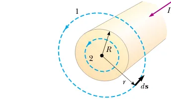
A long, straight wire of radius Rcarries a steady current I that is uniformly distributed through the cross section of the wire (Fig. 30.12). Calculate the magnetic field a distance rfrom the center of the wire in the regions r-R and r.R.
Solution Figure 30.12 helps us to conceptualize the wire and the current. Because the wire has a high degree of symmetry, we categorize this as an Ampère’s law problem. For the r-R case, we should arrive at the same result we obtained in Example 30.1, in which we applied the Biot–Savart law to the same situation. To analyze the problem, let us choose for our path of integration circle 1 in Figure 30.12. From symmetry, B must be constant in magnitude and parallel to ds at every point on this circle. Because the total current passing through the plane of the
Quick Quiz 30.5
Rank the magnitudes of #B(ds for the closed paths in Figure 30.11, from least to greatest.a
b
c
d
Figure 30.11 (Quick Quiz 30.5) Several closed paths near a single current-carrying wire.
Example 30.4 The Magnetic Field Created by a Long Current-Carrying Wire
circle isI, Ampère’s law gives
(for r-R) (30.14)
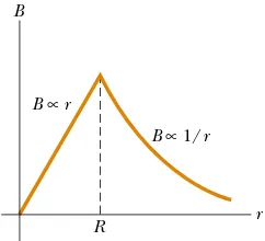
which is identical in form to Equation 30.5. Note how much easier it is to use Ampère’s law than to use the Biot–Savart law. This is often the case in highly symmetric situations.
Now consider the interior of the wire, where r.R. Here the current I%passing through the plane of circle 2 is less than the total current I. Because the current is uniform over the cross section of the wire, the fraction of the current enclosed by circle 2 must equal the ratio of the area $r2 enclosed by circle 2 to the cross-sectional area $R2 of the wire:3
Following the same procedure as for circle 1, we apply Ampère’s law to circle 2:
%
B(ds"B(2$r)"#0I % "#0&
r2 R2 I'
I % " r2
R2 I I%
I " $r2 $R2 #0I 2$r B"
%
B(ds"B%
ds"B(2$r)"#0IFigure 30.12 (Example 30.4) A long, straight wire of radius R carrying a steady current Iuniformly distributed across the cross section of the wire. The magnetic field at any point can be calculated from Ampère’s law using a circular path of radius r, concentric with the wire.
2 R
r
1 I
ds
3 Another way to look at this problem is to realize that the current enclosed by circle 2 must
due to an infinite sheet of charge does not depend on distance from the sheet. Thus, we might expect a similar result here for the magnetic field.
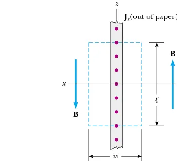
To evaluate the line integral in Ampère’s law, we construct a rectangular path through the sheet, as in Figure 30.15. The rectangle has dimensions !and w, with the sides of length !parallel to the sheet surface. The net current in the plane of the rectangle is Js!. We apply Ampère’s law over the rectangle and note that the two sides of length wdo not contribute to the line integral because the component of B
So far we have imagined currents carried by wires of small cross section. Let us now consider an example in which a current exists in an extended object. A thin, infinitely large sheet lying in the yzplane carries a current of linear current density Js. The current is in the ydirection, and Jsrepresents the current per unit length measured along the zaxis. Find the magnetic field near the sheet.
Solution This situation is similar to those involving Gauss’s law (see Example 24.8). You may recall that the electric field A device called a toroid (Fig. 30.14) is often used to create an almost uniform magnetic field in some enclosed area. The device consists of a conducting wire wrapped around a ring (a torus) made of a nonconducting material. For a toroid having Nclosely spaced turns of wire, calculate the magnetic field in the region occupied by the torus, a distance rfrom the center.
Solution To calculate this field, we must evaluate #B(ds
over the circular amperian loop of radius rin the plane of Figure 30.14. By symmetry, we see that the magnitude of the field is constant on this circle and tangent to it, so B(ds" B ds.Furthermore, the wire passes through the loop Ntimes,
so that the total current through the loop is NI. Therefore, the right side of Equation 30.13 is #0NIin this case.
Ampère’s law applied to the circle gives
(30.16)
This result shows that Bvaries as 1/rand hence is nonuniform in the region occupied by the torus. However, if r is very large compared with the cross-sectional radius aof the torus, then the field is approximately uniform inside the torus.
For an ideal toroid, in which the turns are closely spaced, the external magnetic field is close to zero. It is not exactly zero, however. In Figure 30.14, imagine the radius rof the amperian loop to be either smaller than bor larger than c. In either case, the loop encloses zero net current, so #B(ds"0. We might be tempted to claim that this proves that B"0, but it does not. Consider the amperian loop on the right side of the toroid in Figure 30.14. The plane of this loop is perpen-dicular to the page, and the toroid passes through the loop. As charges enter the toroid as indicated by the current directions in Figure 30.14, they work their way counterclockwise around the toroid. Thus, a current passes through the perpendicular amperian loop! This current is small, but it is not zero. As a result, the toroid acts as a current loop and produces a weak external field of the form shown in Figure 30.7. The reason
Figure 30.14 (Example 30.5) A toroid consisting of many turns of wire. If the turns are closely spaced, the magnetic field in the interior of the torus (the gold-shaded region) is tangent to the dashed circle and varies as 1/r. The dimension ais the cross-sectional radius of the torus. The field outside the toroid is very small and can be described by using the amperian loop at the right side, perpendicular to the page.
Figure 30.13 (Example 30.4) Magnitude of the magnetic field versus rfor the wire shown in Figure 30.12. The field is propor-tional to rinside the wire and varies as 1/routside the wire.
R r
Example 30.5 The Magnetic Field Created by a Toroid
Example 30.6 Magnetic Field Created by an Infinite Current Sheet (30.15)
S E C T I O N 3 0 . 3 • Ampère’s Law 937
Wire 1 in Figure 30.16 is oriented along the y axis and carries a steady current I1. A rectangular loop located to the right of the wire and in the xy plane carries a current I2. Find the magnetic force exerted by wire 1 on the top wire of length bin the loop, labeled “Wire 2” in the figure. the magnetic field created by the current in wire 1 at the position of ds. From Ampère’s law, the field at a distance x Figure 30.15 (Example 30.6) End view of an infinite current sheet lying in the yzplane, where the current is in the y direc-tion (out of the page). This view shows the direcdirec-tion of Bon both sides of the sheet.
Figure 30.16 (Example 30.7) A wire on one side of a rectangu-lar loop lying near a current-carrying wire experiences a force.
from wire 1 (see Eq. 30.14) is
where the unit vector 'kˆis used to indicate that the field due to the current in wire 1 at the position of dspoints into the page. Because wire 2 is along the xaxis, ds"dxˆi, and we find that
Integrating over the limits x"ato x"a*bgives
(1)
The force on wire 2 points in the positive y direction, as indicated by the unit vector ˆjand as shown in Figure 30.16. What If? What if the wire loop is moved to the left in Figure 30.16 until a"0? What happens to the magnitude of the force on the wire?
Answer The force should become stronger because the loop is moving into a region of stronger magnetic field. Equation (1) shows that the force not only becomes stronger but the magnitude of the force becomes infiniteas a:0! Thus, as the loop is moved to the left in Figure 30.16, the loop should be torn apart by the infinite upward force on the top side and the corresponding downward force on the bottom side! Furthermore, the force on the left side is
Example 30.7 The Magnetic Force on a Current Segment
hence the field should not vary from point to point. The only choices of field direction that are reasonable in this situation are either perpendicular or parallel to the sheet. However, a perpendicular field would pass through the current, which is inconsistent with the Biot–Savart law. Assuming a field that is constant in magnitude and parallel to the plane of the sheet, we obtain
This result shows that the magnetic field is independent of distance from the current sheet, as we suspected. The expression for the magnitude of the magnetic field is similar in form to that for the magnitude of the electric field due to an infinite sheet of charge (Example 24.8):
E" /
30.4
The Magnetic Field of a Solenoid
A solenoid is a long wire wound in the form of a helix. With this configuration, a reasonably uniform magnetic field can be produced in the space surrounded by the turns of wire—which we shall call the interior of the solenoid—when the solenoid carries a current. When the turns are closely spaced, each can be approximated as a circular loop, and the net magnetic field is the vector sum of the fields resulting from all the turns.
Figure 30.17 shows the magnetic field lines surrounding a loosely wound solenoid. Note that the field lines in the interior are nearly parallel to one another, are uniformly distributed, and are close together, indicating that the field in this space is strong and almost uniform.
If the turns are closely spaced and the solenoid is of finite length, the magnetic field lines are as shown in Figure 30.18a. This field line distribution is similar to that surrounding a bar magnet (see Fig. 30.18b). Hence, one end of the solenoid behaves like the north pole of a magnet, and the opposite end behaves like the south pole. As the length of the solenoid increases, the interior field becomes more uniform and the exterior field becomes weaker. An ideal solenoid is approached when the turns are closely spaced and the length is much greater than the radius of the turns. Figure 30.19 shows a longitudinal cross section of part of such a solenoid carrying a current I. In this case, the external field is close to zero, and the interior field is uniform over a great volume.
toward the left and should also become infinite. This is larger than the force toward the right on the right side because this side is still far from the wire, so the loop should be pulled into the wire with infinite force!
Does this really happen? In reality, it is impossible for
a:0 because both wire 1 and wire 2 have finite sizes, so that the separation of the centers of the two wires is at least the sum of their radii.
A similar situation occurs when we re-examine the magnetic field due to a long straight wire, given by Equation 30.5. If we could move our observation point infinitesimally close to the wire, the magnetic field would become infinite! But in reality, the wire has a radius, and as soon as we enter the wire, the magnetic field starts to fall off as described by Equation 30.15—approaching zero as we approach the center of the wire.
Exterior
Interior
(a) S N Figure 30.17 The magnetic field
lines for a loosely wound solenoid.
Figure 30.18 (a) Magnetic field lines for a tightly wound solenoid of finite length, carrying a steady current. The field in the interior space is strong and nearly uniform. Note that the field lines resemble those of a bar magnet, meaning that the solenoid effectively has north and south poles. (b) The magnetic field pattern of a bar magnet, displayed with small iron filings on a sheet of paper.
Henry Leap and Jim Lehman
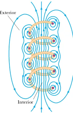
If we consider the amperian loop perpendicular to the page in Figure 30.19, surrounding the ideal solenoid, we see that it encloses a small current as the charges in the wire move coil by coil along the length of the solenoid. Thus, there is a nonzero magnetic field outside the solenoid. It is a weak field, with circular field lines, like those due to a line of current as in Figure 30.4. For an ideal solenoid, this is the only field external to the solenoid. We can eliminate this field in Figure 30.19 by adding a second layer of turns of wire outside the first layer, with the current carried along the axis of the solenoid in the opposite direction compared to the first layer. Then the net current along the axis is zero.
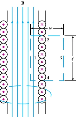
We can use Ampère’s law to obtain a quantitative expression for the interior magnetic field in an ideal solenoid. Because the solenoid is ideal, Bin the interior space is uniform and parallel to the axis, and the magnetic field lines in the exterior space form circles around the solenoid. The planes of these circles are perpendicular to the page. Consider the rectangular path of length ! and width
w shown in Figure 30.19. We can apply Ampère’s law to this path by evaluating the integral of B(ds over each side of the rectangle. The contribution along side 3 is zero because the magnetic field lines are perpendicular to the path in this region. The contributions from sides 2 and 4 are both zero, again because B is perpendicular to ds along these paths, both inside and outside the solenoid. Side 1 gives a contribution to the integral because along this path B is uniform and parallel to ds. The integral over the closed rectangular path is therefore
The right side of Ampère’s law involves the total current I through the area bounded by the path of integration. In this case, the total current through the rectan-gular path equals the current through each turn multiplied by the number of turns. If
Nis the number of turns in the length !, the total current through the rectangle is NI. Therefore, Ampère’s law applied to this path gives
(30.17)
where n"N/!is the number of turns per unit length.
B"#0
N
! I"#0nI
%
B(ds"B!"#0NI%
B(ds"!
path1
B(ds"B
!
path1
ds"B!
S E C T I O N 3 0 . 4 • The Magnetic Field of a Solenoid 939
B
× × × × × × × ×
×
3 2
4
1 !
w
× ×
Figure 30.19 Cross-sectional view of an ideal solenoid, where the interior magnetic field is uniform and the exterior field is close to zero. Ampère’s law applied to the circular path near the bottom whose plane is perpendicular to the page can be used to show that there is a weak field outside the solenoid. Ampère’s law applied to the rectangular dashed path in the plane of the page can be used to calculate the magnitude of the interior field.
30.5
Magnetic Flux
The flux associated with a magnetic field is defined in a manner similar to that used to define electric flux (see Eq. 24.3). Consider an element of area dA on an arbitrarily shaped surface, as shown in Figure 30.20. If the magnetic field at this element is B, the magnetic flux through the element is B(dA, where dAis a vector that is perpendicular to the surface and has a magnitude equal to the area d A. Therefore, the total magnetic flux 1Bthrough the surface is
(30.18)
Consider the special case of a plane of area Ain a uniform field B that makes an angle !with dA. The magnetic flux through the plane in this case is
(30.19)
If the magnetic field is parallel to the plane, as in Figure 30.21a, then ! "90°and the flux through the plane is zero. If the field is perpendicular to the plane, as in Figure 30.21b, then ! "0 and the flux through the plane is BA(the maximum value).
The unit of magnetic flux is T(m2, which is defined as a weber (Wb); 1 Wb" 1 T(m2.
1B"BA cos !
1B"
!
B(dAWe also could obtain this result by reconsidering the magnetic field of a toroid (see Example 30.5). If the radius rof the torus in Figure 30.14 containing N turns is much greater than the toroid’s cross-sectional radius a, a short section of the toroid approximates a solenoid for which n"N/2$r.In this limit, Equation 30.16 agrees with Equation 30.17.
Equation 30.17 is valid only for points near the center (that is, far from the ends) of a very long solenoid. As you might expect, the field near each end is smaller than the value given by Equation 30.17. At the very end of a long solenoid, the magnitude of the field is half the magnitude at the center (see Problem 32).
Quick Quiz 30.6
Consider a solenoid that is very long compared to the radius. Of the following choices, the most effective way to increase the magnetic field in the interior of the solenoid is to (a) double its length, keeping the number of turns per unit length constant, (b) reduce its radius by half, keeping the number of turns per unit length constant, (c) overwrapping the entire solenoid with an additional layer of current-carrying wire.B
dA
θ
Figure 30.20 The magnetic flux through an area element d Ais
B(dA"B d Acos !, where dAis a vector perpendicular to the surface.
(a) (b)
B
dA
B
dA
Active Figure 30.21Magnetic flux through a plane lying in a magnetic field. (a) Theflux through the plane is zero when the magnetic field is parallel to the plane surface. (b) The flux through the plane is a maximum when the magnetic field is perpendicular to the plane.
30.6
Gauss’s Law in Magnetism
In Chapter 24 we found that the electric flux through a closed surface surrounding a net charge is proportional to that charge (Gauss’s law). In other words, the number of electric field lines leaving the surface depends only on the net charge within it. This property is based on the fact that electric field lines originate and terminate on electric charges.
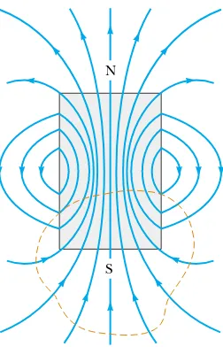
The situation is quite different for magnetic fields, which are continuous and form closed loops. In other words, magnetic field lines do not begin or end at any point—as illustrated in Figures 30.4 and 30.23. Figure 30.23 shows the magnetic field lines of a bar magnet. Note that for any closed surface, such as the one outlined by the dashed line in Figure 30.23, the number of lines entering the surface equals the number leaving the surface; thus, the net magnetic flux is zero. In contrast, for a closed surface surrounding one charge of an electric dipole (Fig. 30.24), the net electric flux is not zero.
Gauss’s law in magnetismstates that
S E C T I O N 3 0 . 6 • Gauss’s Law in Magnetism 941
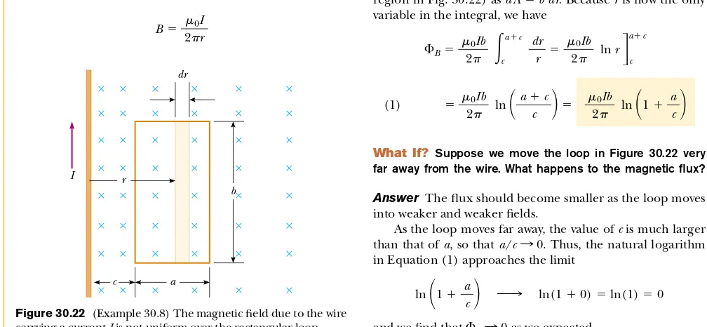
A rectangular loop of width aand length bis located near a long wire carrying a current I (Fig. 30.22). The distance between the wire and the closest side of the loop is c. The wire is parallel to the long side of the loop. Find the total magnetic flux through the loop due to the current in the wire.
Solution From Equation 30.14, we know that the magni-tude of the magnetic field created by the wire at a distance r
from the wire is
B" #0I 2$r
The factor 1/rindicates that the field varies over the loop, and Figure 30.22 shows that the field is directed into the page at the location of the loop. Because Bis parallel to dA
at any point within the loop, the magnetic flux through an area element d Ais
To integrate, we first express the area element (the tan region in Fig. 30.22) as d A"b dr.Because ris now the only variable in the integral, we have
What If? Suppose we move the loop in Figure 30.22 very far away from the wire. What happens to the magnetic flux?
Answer The flux should become smaller as the loop moves into weaker and weaker fields.
As the loop moves far away, the value of cis much larger than that of a, so that a/c:0. Thus, the natural logarithm in Equation (1) approaches the limit
and we find that1B:0 as we expected.
ln
&
1* ac
'
9: ln(1*0)"ln(1)"0#0Ib
2$ ln
&
1*a c
'
(1)
" #0Ib 2$ ln
&
a*c c
'
"1B" #0Ib 2$
!
a*c
c
dr r "
#0Ib 2$ ln r
(
a*c
c
1B"
!
BdA"!
#0I 2$r dAExample 30.8 Magnetic Flux Through a Rectangular Loop Interactive
b r
I
c a dr
× × × × × ×
× × × × × ×
× × × × × ×
× × × × × ×
× × × × × ×
× × × × × ×
× × × × × ×
× × × × × ×
Figure 30.22 (Example 30.8) The magnetic field due to the wire carrying a current Iis not uniform over the rectangular loop.
At the Interactive Worked Example link at http://www.pse6.com,you can investigate the flux as the loop parameters change.
the net magnetic flux through any closed surface is always zero:
(30.20)
This statement is based on the experimental fact, mentioned in the opening of Chapter 29, that isolated magnetic poles (monopoles) have never been detected and perhaps do not exist. Nonetheless, scientists continue the search because certain theo-ries that are otherwise successful in explaining fundamental physical behavior suggest the possible existence of monopoles.
30.7
Displacement Current and the General
Form of Ampère’s Law
We have seen that charges in motion produce magnetic fields. When a current-carrying conductor has high symmetry, we can use Ampère’s law to calculate the magnetic field it creates. In Equation 30.13, #B(ds"#0I, the line integral is over any closed path through which the conduction current passes, where the conduction current is defined by the expression I"dq/dt. (In this section we use the term
conduction current to refer to the current carried by the wire, to distinguish it from a new type of current that we shall introduce shortly.) We now show that Ampère’s law in this form is valid only if any electric fields present are constant in time. Maxwell recognized this limitation and modified Ampère’s law to include time-varying electric fields.
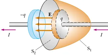
We can understand the problem by considering a capacitor that is being charged as illustrated in Figure 30.25. When a conduction current is present, the charge on the positive plate changes but no conduction current exists in the gap between the plates. Now consider the two surfaces S1 and S2in Figure 30.25, bounded by the same path P. Ampère’s law states that #B(ds around this path must equal #0I, where Iis the total current through anysurface bounded by the path P.
When the path P is considered as bounding S1, #B(ds"#0I because the conduction current passes through S1. When the path is considered as bounding S2, however, #B(ds"0 because no conduction current passes through S2. Thus, we have a contradictory situation that arises from the discontinuity of the current! Maxwell solved this problem by postulating an additional term on the right side N
S
Figure 30.23 The magnetic field lines of a bar magnet form closed loops. Note that the net magnetic flux through a closed surface surrounding one of the poles (or any other closed surface) is zero. (The dashed line represents the intersection of the surface with the page.)
–
+
Figure 30.24 The electric field lines surrounding an electric dipole begin on the positive charge and terminate on the negative charge. The electric flux through a closed surface surrounding one of the charges is not zero.
Path P
A –q
S1
S2 q
I
of Equation 30.13, which includes a factor called the displacement current Id,
defined as4
(30.21)
where 00is the permittivity of free space (see Section 23.3) and is the electric flux (see Eq. 24.3).
As the capacitor is being charged (or discharged), the changing electric field between the plates may be considered equivalent to a current that acts as a continuation of the conduction current in the wire. When the expression for the displacement current given by Equation 30.21 is added to the conduction current on the right side of Ampère’s law, the difficulty represented in Figure 30.25 is resolved. No matter which surface bounded by the path P is chosen, either a conduction current or a displacement current passes through it. With this new term
Id, we can express the general form of Ampère’s law (sometimes called the
Ampère–Maxwell law) as5
(30.22)
We can understand the meaning of this expression by referring to Figure 30.26. The electric flux through surface S2 is , where A is the area of the capacitor plates and E is the magnitude of the uniform electric field between the plates. If q is the charge on the plates at any instant, then E"q/(00A). (See Section 26.2.) Therefore, the electric flux through S2is simply
Hence, the displacement current through S2is
(30.23)
That is, the displacement current Id through S2 is precisely equal to the conduction current Ithrough S1!
Id"00
d1E
dt " dq dt
1E"EA" q 00 12"!E(dA"23
%
B(ds"#0(I*Id)"#0I*#000d1E
dt
12"!E(dA
Id)00 d1E
dt
S E C T I O N 3 0 . 7 • Displacement Current and the General Form of Ampère’s Law 943
Ampère–Maxwell law Displacement current
4 Displacementin this context does not have the meaning it does in Chapter 2. Despite the
inaccurate implications, the word is historically entrenched in the language of physics, so we continue to use it.
5 Strictly speaking, this expression is valid only in a vacuum. If a magnetic material is present,
one must change#0and 00on the right-hand side of Equation 30.22 to the permeability #m(see
Section 30.8) and permittivity 0characteristic of the material. Alternatively, one may include a magnetizing current Imon the right hand side of Equation 30.22 to make Ampère’s law fully
general. On a microscopic scale, Imis as real as I.
E
–q
S2 S1
q
I I
Figure 30.26 Because it exists only in the wires attached to the capacitor plates, the conduction current I"dq/dtpasses through S1but not through S2. Only the
A sinusoidally varying voltage is applied across an 8.00-#F capacitor. The frequency of the voltage is 3.00 kHz, and the voltage amplitude is 30.0 V. Find the displacement current in the capacitor.
Solution The angular frequency of the source, from Equation 15.12, is given by 4 "2$f"2$(3.00&103Hz)" 1.88&104s'1. Hence, the voltage across the capacitor in terms oftis
5V" 5Vmaxsin 4t"(30.0 V) sin(1.88&104t) We can use Equation 30.23 and the fact that the charge on the capacitor is q"C5V to find the displacement
By considering surface S2, we can identify the displacement current as the source of the magnetic field on the surface boundary. The displacement current has its physical origin in the time-varying electric field. The central point of this formalism is that
Quick Quiz 30.7
In an RCcircuit, the capacitor begins to discharge. During the discharge, in the region of space between the plates of the capacitor, there is (a) conduction current but no displacement current, (b) displacement current but no conduction current, (c) both conduction and displacement current, (d) no current of any type.Quick Quiz 30.8
The capacitor in an RCcircuit begins to discharge. During the discharge, in the region of space between the plates of the capacitor, there is (a) an electric field but no magnetic field, (b) a magnetic field but no electric field, (c) both electric and magnetic fields, (d) no fields of any type.magnetic fields are produced both by conduction currents and by time-varying electric fields.
current:
The displacement current varies sinusoidally with time and has a maximum value of 4.52 A.
(4.52 A) cos(1.88&104t) "
"(8.00&10'6 F) d
dt [(30.0 V) sin(1.88&10
4t)]
Id"
dq dt "
d
dt (C∆V)"C d dt (∆V)
Example 30.9 Displacement Current in a Capacitor
This result was a remarkable example of theoretical work by Maxwell, and it contributed to major advances in the understanding of electromagnetism.
30.8
Magnetism in Matter
The magnetic field produced by a current in a coil of wire gives us a hint as to what causes certain materials to exhibit strong magnetic properties. Earlier we found that a coil like the one shown in Figure 30.18 has a north pole and a south pole. In general,
anycurrent loop has a magnetic field and thus has a magnetic dipole moment, includ-ing the atomic-level current loops described in some models of the atom.
The Magnetic Moments of Atoms
S E C T I O N 3 0 . 8 • Magnetism in Matter 945
and the magnetic moment of the electron is associated with this orbital motion. Although this model has many deficiencies, some of its predictions are in good agreement with the correct theory, which is expressed in terms of quantum physics.
In our classical model, we assume that an electron moves with constant speed vin a circular orbit of radius rabout the nucleus, as in Figure 30.27. Because the electron travels a distance of 2$r (the circumference of the circle) in a time interval T, its orbital speed is v"2$r/T. The current Iassociated with this orbiting electron is its charge edivided by T. Using T"2$/4and 4 "v/r, we have
The magnitude of the magnetic moment associated with this current loop is # "IA,
where A"$r2is the area enclosed by the orbit. Therefore,
(30.24)
Because the magnitude of the orbital angular momentum of the electron is L"mevr
(Eq. 11.12 with 6 "90°), the magnetic moment can be written as
(30.25)
This result demonstrates that the magnetic moment of the electron is proportional to its orbital angular momentum. Because the electron is negatively charged, the vectors "and Lpoint in oppositedirections. Both vectors are perpendicular to the plane of the orbit, as indicated in Figure 30.27.
A fundamental outcome of quantum physics is that orbital angular momentum is quantized and is equal to multiples of "h/2$ "1.05&10'34J(s, where h is Planck’s constant (introduced in Section 11.6). The smallest nonzero value of the electron’s magnetic moment resulting from its orbital motion is
(30.26)
We shall see in Chapter 42 how expressions such as Equation 30.26 arise.
Because all substances contain electrons, you may wonder why most substances are not magnetic. The main reason is that in most substances, the magnetic moment of one electron in an atom is canceled by that of another electron orbiting in the opposite direction. The net result is that, for most materials, the magnetic effect produced by the orbital motion of the electrons is either zero or very small.
In addition to its orbital magnetic moment, an electron (as well as protons, neutrons, and other particles) has an intrinsic property called spin that also contributes to its magnetic moment. Classically, the electron might be viewed as
# "
√
2 e 2me7 7 # "
&
e2me
'
L# "IA"
&
ev 2$r'
$r2"1 2evr
I" e
T " e4 2$ "
e v
2$r
Orbital magnetic moment r
µ L
Figure 30.27 An electron moving in the direction of the gray arrow in a circular orbit of radius rhas an angular momentum
Lin one direction and a magnetic moment "in the opposite direction. Because the electron carries a negative charge, the direction of the current due to its motion about the nucleus is opposite the direction of that motion.
▲
PITFALL PREVENTION
30.3
The Electron Does
Not Spin
Do not be misled; the electron is
spinning about its axis as shown in Figure 30.28, but you should be very careful with the classical interpretation. The magnitude of the angular momentum S associated with spin is on the same order of magnitude as the magnitude of the angular momen-tum Ldue to the orbital motion. The magnitude of the spin angular momentum of an electron predicted by quantum theory is
The magnetic moment characteristically associated with the spin of an electron has the value
(30.27)
This combination of constants is called the Bohr magneton"B:
(30.28)
Thus, atomic magnetic moments can be expressed as multiples of the Bohr magneton. (Note that 1 J/T"1 A(m2.)
In atoms containing many electrons, the electrons usually pair up with their spins opposite each other; thus, the spin magnetic moments cancel. However, atoms containing an odd number of electrons must have at least one unpaired electron and therefore some spin magnetic moment. The total magnetic moment of an atom is the vector sum of the orbital and spin magnetic moments, and a few examples are given in Table 30.1. Note that helium and neon have zero moments because their individual spin and orbital moments cancel.
The nucleus of an atom also has a magnetic moment associated with its constituent protons and neutrons. However, the magnetic moment of a proton or neutron is much smaller than that of an electron and can usually be neglected. We can understand this by inspecting Equation 30.28 and replacing the mass of the electron with the mass of a proton or a neutron. Because the masses of the proton and neutron are much greater than that of the electron, their magnetic moments are on the order of 103 times smaller than that of the electron.
Magnetization Vector and Magnetic Field Strength
The magnetic state of a substance is described by a quantity called the magnetization vector M. The magnitude of this vector is defined as the magnetic moment per unit volume of the substance. As you might expect, the total magnetic field B at a point within a substance depends on both the applied (external) field B0 and the magnetization of the substance.
Consider a region in which a magnetic field B0is produced by a current-carrying conductor. If we now fill that region with a magnetic substance, the total magnetic field B in the region is B"B0*Bm, where Bm is the field produced by the magnetic
substance.
Let us determine the relationship between Bmand M. Imagine that the field Bmis
created by a solenoid rather than by the magnetic material. Then, Bm"#0nI, where I is the current in the imaginary solenoid and nis the number of turns per unit length. Let us manipulate this expression as follows:
where Nis the number of turns in length !, and we have multiplied the numerator and denominator by A, the cross sectional area of the solenoid in the last step. We recognize the numerator NIA as the total magnetic moment of all the loops in
Bm"#0nI"#0
N
! I"#0
NIA
!A #B"
e7 2me
"9.27&10'24J/T #spin" e7
2me
S"
√
3 2 7Magnetization vector M
spin
µ
Figure 30.28 Classical model of a spinning electron. We can adopt this model to remind ourselves that electrons have an intrinsic angular momentum. The model should not be pushed too far, however—it gives an incorrect magnitude for the magnetic moment, incorrect quantum numbers, and too many degrees of freedom.
Magnetic Moment Atom or Ion (10#24J/T)
H 9.27
He 0
Ne 0
Ce3* 19.8
Yb3* 37.1
Magnetic Moments of Some Atoms and Ions
length !and the denominator !Aas the volume of the solenoid associated with this length:
The ratio of total magnetic moment to volume is what we have defined as magnetiza-tion in the case where the field is due to a material rather than a solenoid. Thus, we can express the contribution Bmto the total field in terms of the magnetization vector of the substance as Bm"#0M. When a substance is placed in a magnetic field, the total magnetic field in the region is expressed as
(30.29)
When analyzing magnetic fields that arise from magnetization, it is convenient to introduce a field quantity called the magnetic field strength Hwithin the substance. The magnetic field strength is related to the magnetic field due to the conduction currents in wires. To emphasize the distinction between the field strength Hand the field B, the latter is often called the magnetic flux densityor the magnetic induction.The magnetic field strength is the magnetic moment per unit volume due to currents; thus, it is similar to the vector Mand has the same units.
Recognizing the similarity between M and H, we can define H as H)B0/#0. Thus, Equation 30.29 can be written
(30.30)
The quantities Hand Mhave the same units. Because Mis magnetic moment per unit volume, its SI units are (ampere)(meter)2/(meter)3, or amperes per meter.
To better understand these expressions, consider the torus region of a toroid that carries a current I. If this region is a vacuum, M"0 (because no magnetic material is present), the total magnetic field is that arising from the current alone, and B"B0"
#0H. Because B0"#0nIin the torus region, where nis the number of turns per unit length of the toroid, H"B0/#0"#0nI/#0or
(30.31)
In this case, the magnetic field in the torus region is due only to the current in the windings of the toroid.
If the torus is now made of some substance and the current Iis kept constant, Hin the torus region remains unchanged (because it depends on the current only) and has magnitude nI. The total field B, however, is different from that when the torus region was a vacuum. From Equation 30.30, we see that part of Barises from the term #0Hassociated with the current in the toroid, and part arises from the term #0M due to the magnetization of the substance of which the torus is made.
Classification of Magnetic Substances
Substances can be classified as belonging to one of three categories, depending on their magnetic properties. Paramagnetic and ferromagnetic materials are those made of atoms that have permanent magnetic moments. Diamagneticmaterials are those made of atoms that do not have permanent magnetic moments.
For paramagnetic and diamagnetic substances, the magnetization vector M is proportional to the magnetic field strength H. For these substances placed in an external magnetic field, we can write
(30.32)
where 8(Greek letter chi) is a dimensionless factor called the magnetic susceptibil-ity.It can be considered a measure of how susceptiblea material is to being magnetized. For paramagnetic substances, 8is positive and Mis in the same direction as H. For
M"8H
H"nI
B"#0(H*M) B"B0*#0M
Bm"#0 #
V
S E C T I O N 3 0 . 8 • Magnetism in Matter 947
Magnetic field strength H