123
LNCS 8115
19th EUNICE/IFIP WG 6.6 International Workshop
Chemnitz, Germany, August 2013
Proceedings
Advances
Commenced Publication in 1973 Founding and Former Series Editors:
Gerhard Goos, Juris Hartmanis, and Jan van Leeuwen
Editorial Board
David Hutchison
Lancaster University, UK Takeo Kanade
Carnegie Mellon University, Pittsburgh, PA, USA Josef Kittler
University of Surrey, Guildford, UK Jon M. Kleinberg
Cornell University, Ithaca, NY, USA Alfred Kobsa
University of California, Irvine, CA, USA Friedemann Mattern
ETH Zurich, Switzerland John C. Mitchell
Stanford University, CA, USA Moni Naor
Weizmann Institute of Science, Rehovot, Israel Oscar Nierstrasz
University of Bern, Switzerland C. Pandu Rangan
Indian Institute of Technology, Madras, India Bernhard Steffen
TU Dortmund University, Germany Madhu Sudan
Microsoft Research, Cambridge, MA, USA Demetri Terzopoulos
University of California, Los Angeles, CA, USA Doug Tygar
University of California, Berkeley, CA, USA Gerhard Weikum
Advances
in Communication
Networking
19th EUNICE/IFIP WG 6.6 International Workshop
Chemnitz, Germany, August 28-30, 2013
Proceedings
Thomas Bauschert
Technische Universität Chemnitz Professur Kommunikationsnetze Reichenhainer Straße 70 09107 Chemnitz, Germany
E-mail: [email protected] Web: http://www.tu-chemnitz.de/etit/kn/
ISSN 0302-9743 e-ISSN 1611-3349
ISBN 978-3-642-40551-8 e-ISBN 978-3-642-40552-5 DOI 10.1007/978-3-642-40552-5
Springer Heidelberg New York Dordrecht London
Library of Congress Control Number: 2013946103
CR Subject Classification (1998): C.2.0-2, C.2, H.3.3-5, F.2.2, C.0, K.6, H.4
LNCS Sublibrary: SL 3 – Information Systems and Application, incl. Internet/Web and HCI
© IFIP International Federation for Information Processing 2013
This work is subject to copyright. All rights are reserved by the Publisher, whether the whole or part of the material is concerned, specifically the rights of translation, reprinting, reuse of illustrations, recitation, broadcasting, reproduction on microfilms or in any other physical way, and transmission or information storage and retrieval, electronic adaptation, computer software, or by similar or dissimilar methodology now known or hereafter developed. Exempted from this legal reservation are brief excerpts in connection with reviews or scholarly analysis or material supplied specifically for the purpose of being entered and executed on a computer system, for exclusive use by the purchaser of the work. Duplication of this publication or parts thereof is permitted only under the provisions of the Copyright Law of the Publisher’s location, in its current version, and permission for use must always be obtained from Springer. Permissions for use may be obtained through RightsLink at the Copyright Clearance Center. Violations are liable to prosecution under the respective Copyright Law.
The use of general descriptive names, registered names, trademarks, service marks, etc. in this publication does not imply, even in the absence of a specific statement, that such names are exempt from the relevant protective laws and regulations and therefore free for general use.
While the advice and information in this book are believed to be true and accurate at the date of publication, neither the authors nor the editors nor the publisher can accept any legal responsibility for any errors or omissions that may be made. The publisher makes no warranty, express or implied, with respect to the material contained herein.
Typesetting:Camera-ready by author, data conversion by Scientific Publishing Services, Chennai, India Printed on acid-free paper
It was a great honor for TU Chemnitz to host the 19th EUNICE Workshop on Advances in Communication Networking. EUNICE has a long tradition in bringing together young scientists and researchers from academia, industry, and government organizations to meet and to discuss their recent achievements. The single-track structure with sufficient time for presentations provides an excellent platform for stimulating discussions. The proceedings of the EUNICE workshops are published in Springer’s LNCS series.
This year, the workshop focus was on “Advances in Communication Network-ing.” Several keynote speakers from industry were invited to foster discussions between industry and academia about recent communication networking issues, trends, and solutions. Moreover, the original aim of the EUNICE-Forum was adopted by organizing a summer school on the dedicated topic of “Network Per-formance Evaluation and Optimization” co-located to the EUNICE workshop.
EUNICE 2013 received 40 paper submissions. According to the evaluations, the top 23 papers were selected for oral presentations. In addition, nine papers were selected for poster presentations. All of these papers appear in this pro-ceedings volume.
On behalf of the Chair for Communication Networks of TU Chemnitz, I would like to express my thanks to everyone who actively participated in the organization of EUNICE 2013, in particular to the members of the Technical Program Committee, the reviewers, and last but not least the members of my team. Special thanks go to the keynote speakers from industry for contributing to the workshop as well as to the colleagues from academia for contributing to the summer school.
EUNICE 2013 was organized by the Chair for Communication Networks, TU Chemnitz.
Executive Committee
Conference Chair
Thomas Bauschert Chair for Communication Networks, TU Chemnitz, Germany
Local Organization
Thomas M. Knoll TU Chemnitz, Germany
Technical Program Committee
Finn Arve Aagesen NTNU Trondheim, Norway Thomas Bauschert TU Chemnitz, Germany
Piotr Cholda AGH University Krakow, Poland J¨org Ebersp¨acher TU M¨unchen, Germany
Markus Fiedler BIT, Blekinge, Sweden
Carmelita G¨org University of Bremen, Germany Annie Gravey TELECOM Bretagne, France Yvon Kermarrec TELECOM Bretagne, France Thomas M. Knoll TU Chemnitz, Germany
Paul K¨uhn University of Stuttgart, Germany Ralf Lehnert TU Dresden, Germany
Matthias Lott DOCOMO Euro-Labs M¨unchen, Germany Miquel Oliver University Pompeu Fabra, Spain
Michal Pioro Warsaw University of Technology, Poland Aiko Pras University of Twente, The Netherlands Jacek Rak Gdansk University of Technology, Poland Burkhard Stiller University of Z¨urich, Switzerland
Robert Szabo Budapest University of Technology, Hungary Andreas Timm-Giel TU Hamburg-Harburg, Germany
Phuoc Tran-Gia University of W¨urzburg, Germany Christian Wietfeld TU Dortmund, Germany
Sponsors
•EUNICE
•International Federation for Information Processing (IFIP)
•Informationstechnische Gesellschaft (ITG) im VDE
Network Modeling and Design
Dynamic Resource Operation and Power Model for IP-over-WSON
Networks . . . 1
Uwe Bauknecht and Frank Feller
A Generic Multi-layer Network Optimization Model with Demand
Uncertainty . . . 13
Uwe Steglich, Thomas Bauschert, Christina B¨using, and Manuel Kutschka
Modeling and Quantifying the Survivability of Telecommunication
Network Systems under Fault Propagation. . . 25
Lang Xie, Poul E. Heegaard, and Yuming Jiang
Traffic Analysis
Analysis of Elephant Users in Broadband Network Traffic. . . 37
P´eter Megyesi and S´andor Moln´ar
Evaluation of the Aircraft Distribution in Satellite Spotbeams . . . 46
Christoph Petersen, Maciej M¨uhleisen, and Andreas Timm-Giel
Network and Traffic Management
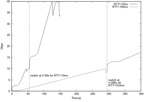
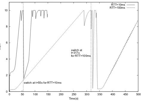
Self-management of Hybrid Networks – Hidden Costs Due to TCP
Performance Problems. . . 54
Giovane C.M. Moura, Aiko Pras, Tiago Fioreze, and Pieter-Tjerk de Boer
A Revenue-Maximizing Scheme for Radio Access Technology Selection
in Heterogeneous Wireless Networks with User Profile Differentiation. . . 66
Elissar Khloussy, Xavier Gelabert, and Yuming Jiang
Services over Mobile Networks
Mobile SIP: An Empirical Study on SIP Retransmission Timers
in HSPA 3G Networks. . . 78
Addressing the Challenges of E-Healthcare in Future Mobile
Networks . . . 90
Safdar Nawaz Khan Marwat, Thomas P¨otsch, Yasir Zaki, Thushara Weerawardane, and Carmelita G¨org
Monitoring and Measurement
Evaluation of Video Quality Monitoring Based on Pre-computed Frame
Distortions. . . 100
Dominik Klein, Thomas Zinner, Kathrin Borchert, Stanislav Lange, Vlad Singeorzan, and Matthias Schmid
QoE Management Framework for Internet Services in SDN Enabled
Mobile Networks. . . 112
Marcus Eckert and Thomas Martin Knoll
A Measurement Study of Active Probing on Access Links. . . 124
Bjørn J. Villa and Poul E. Heegaard
Design and Evaluation of HTTP Protocol Parsers for IPFIX
Measurement. . . 136
Petr Velan, Tom´aˇs Jirs´ık, and Pavel ˇCeleda
Security Concepts
IPv6 Address Obfuscation by Intermediate Middlebox in Coordination
with Connected Devices . . . 148
Florent Fourcot, Laurent Toutain, Stefan K¨opsell, Fr´ed´eric Cuppens, and Nora Cuppens-Boulahia
Balanced XOR-ed Coding. . . 161
Katina Kralevska, Danilo Gligoroski, and Harald Øverby
Application of ICT in Smart Grid
and Smart Home Environments
Architecture and Functional Framework for Home Energy Management
Systems . . . 173
Kornschnok Dittawit and Finn Arve Aagesen
Interdependency Modeling in Smart Grid and the Influence of ICT
on Dependability . . . 185
Jonas W¨afler and Poul E. Heegaard
Development and Calibration of a PLC Simulation Model
for UPA-Compliant Networks. . . 197
Data Dissemination in Ad-Hoc and Sensor Networks
Efficient Data Aggregation with CCNx in Wireless Sensor Networks. . . . 209
Torsten Teubler, Mohamed Ahmed M. Hail, and Horst Hellbr¨uck
EpiDOL: Epidemic Density Adaptive Data Dissemination Exploiting
Opposite Lane in VANETs. . . 221
Irem Nizamoglu, Sinem Coleri Ergen, and Oznur Ozkasap
Services and Applications
Advanced Approach to Future Service Development. . . 233
Tetiana Kot, Larisa Globa, and Alexander Schill
A Transversal Alignment between Measurements and Enterprise
Architecture for Early Verification of Telecom Service Design. . . 245
Iyas Alloush, Yvon Kermarrec, and Siegfried Rouvrais
DOMINO – An Efficient Algorithm for Policy Definition and Processing
in Distributed Environments Based on Atomic Data Structures . . . 257
Joachim Zeiß, Peter Reichl, Jean-Marie Bonnin, and J¨urgen Dorn
Poster Papers
Performance Evaluation of Machine-to-Machine Communication on
Future Mobile Networks in Disaster Scenarios . . . 270
Thomas P¨otsch, Safdar Nawaz Khan Marwat, Yasir Zaki, and Carmelita G¨org
Notes on the Topological Consequences of BGP Policy Routing on the
Internet AS Topology. . . 274
D´avid Szab´o and Andr´as Guly´as
Graph-Theoretic Roots of Value Network Quantification . . . 282
Patrick Zwickl and Peter Reichl
A Publish-Subscribe Scheme Based Open Architecture
for Crowd-Sourcing . . . 287
R´obert L. Szab´o and K´aroly Farkas
A Testbed Evaluation of the Scalability of IEEE 802.11s Light
Sleep Mode . . . 292
Marco Porsch and Thomas Bauschert
HTTP Traffic Offload in Cellular Networks via WLAN Mesh Enabled
Device to Device Communication and Distributed Caching . . . 298
Protocol-Independent Detection of Dictionary Attacks. . . 304
Martin Draˇsar
Distributing Key Revocation Status in Named Data Networking . . . 310
Giulia Mauri and Giacomo Verticale
Test-Enhanced Life Cycle for Composed IoT-Based Services. . . 314
Daniel Kuemper, Eike Steffen Reetz, Daniel H¨olker, and Ralf T¨onjes
for IP-over-WSON Networks
Uwe Bauknecht and Frank Feller
Institute of Communication Networks and Computer Engineering (IKR) Universit¨at Stuttgart, Pfaffenwaldring 47, 70569 Stuttgart, Germany
{uwe.bauknecht,frank.feller}@ikr.uni-stuttgart.de
Abstract. The power consumption of core networks is bound to grow considerably due to increasing traffic volumes. Network reconfiguration adapting resources to the load is a promising countermeasure. However, the benefit of this approach is hard to evaluate realistically since current network equipment does not support dynamic resource adaptation and power-saving features. In this paper, we derive a dynamic resource op-eration and power model for IP-over-WSON network devices based on static power consumption data from vendors and reasonable assumptions on the achievable scaling behavior. Our model allows to express the dy-namic energy consumption as a function of active optical interfaces, line cards, chassis, and the amount of switched IP traffic. We finally apply the model in the evaluation of two network reconfiguration schemes.
Keywords: Dynamic Energy Model, Resource Model, IP-over-WDM Network, Multi-layer Network, Energy Efficiency.
1
Introduction
The continuous exponential growth of the traffic volume is driving an increase in the power consumption of communication networks, which has gained im-portance due to economic, environmental, and regulatory considerations. While the access segment has traditionally accounted for the largest share of the en-ergy consumed in communication networks, core networks are bound to be-come predominant due to new energy-efficient broadband access technologies like FTTx [1,2].
Today, core network resources are operated statically whereas the traffic ex-hibits significant variations over the day, including night periods with as little as 20 % of the daily peak rate [3]. Adapting the amount of active, i. e. energy-consuming, resources to the traffic load could therefore significantly reduce power consumption. Since the paradigm of static operation has traditionally guaranteed the reliability of transport networks, research needs to thoroughly investigate both the benefits and the consequences of dynamic resource operation.
A first challenge is to determine the energy savings achievable by this ap-proach. Current core network equipment neither allows the deactivation of com-ponents nor features state-of-the-art power-saving techniques (such as frequency
T. Bauschert (Ed.): EUNICE 2013, LNCS 8115, pp. 1–12, 2013. c
scaling found in desktop processors). Hence, its power consumption hardly de-pends on the traffic load [4,5]. For the static operation of network equipment, researchers have derived power models from measurements [4] and product spec-ifications or white papers [6]. These models are either intended as a reference for future research [6] or applied in power-efficient network planning studies [7].
Core network reconfiguration studies base on different power adaptation as-sumptions. Mostly, components (e. g. optical cross-connects, amplifiers, regen-erators [8,9]; router interfaces, line cards [10,11]) or whole links and nodes [10] are switched off. Alternatively, the energy consumption is scaled with active ca-pacity [12], link bit rate [13], or traffic load [14]. Restrepo et al. [15] propose load-dependent energy profiles justified by different power-saving techniques for components and also apply them to nodes. Langeet al. [16] derive a dynamic power model from a generic network device structure and validate it by mea-surements of one piece of power-saving enabled equipment. To our knowledge, however, there is no coherent reference model for the dynamic power consump-tion of current core network equipment assuming state-of-the-art power-scaling techniques. Such a model is highly desirable for network reconfiguration studies. In this paper, we derive a dynamic resource operation and power model for Internet protocol (IP) over wavelength switched optical network (WSON) net-works. We start by decomposing network nodes into their relevant hardware components, for which we obtain static power consumption values from refer-ence models and publicly available manufacturer data. Based on their struc-ture and functions, we identify applicable activation/deactivation patterns and power-scaling techniques and derive the operation state-dependent power con-sumption. We then aggregate the component behavior into a power model suit-able for network-level studies. It features power values for optical circuits and electrically switched traffic. In addition, it takes the resource hierarchy of net-work nodes into consideration and describes their static power consumption. We finally illustrate the application of our model using reconfiguration schemes from [11,17].
2
Network Equipment Structure
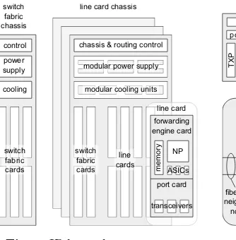
The two layers of IP-over-WSON networks are reflected in the structure of the network nodes. The nodes typically consist of a router processing IP packets for the upper layer and a wavelength-selective optical circuit switch in the lower layer. Optical circuits interconnect arbitrary IP routers.
2.1 IP Routers
Fig. 1.IP layer device structure
Fig. 2.WSON node structure
are managed by the chassis control (CC) among other tasks. The routing engine (RE) exchanges routing protocol messages with other network nodes and builds a routing table. Essentially, the CC and RE modules are small general-purpose server systems. In the case of Cisco, one such system fulfills both functions.
Line cards (LC) perform the central role of the router: they terminate optical circuits and switch the traffic on the IP packet level. One can subdivide them according to these functions into port cards (PC) and forwarding engine cards (FE). The latter feature network processors (NP), further application specific integrated circuits (ASIC), and memory to process and store packets. NPs gen-erally have highly parallel architectures1. Typically, one part of the memory is used for packet buffering, whereas a copy of the routing table occupies the rest. PCs provide the connection between optical circuits and the electrical inter-faces of FEs. One PC may terminate several circuits. Traditionally, PCs feature ports for pluggable optical transceiver (transmitter and receiver) modules such as SFP2, XFP3, or CFP4. These transceivers (TRX) are so-called short-reach transceivers (SR-TRX) of a limited optical reach (100 m to 100 km); they con-nect the LCs to transponders (TXP) converting the signal to a given wavelength for long-haul transmission. Alternatively, PCs can directly featurecolored inter-faces with long-reach transceivers (LR-TRX). This avoids the overhead of signal conversion, but currently restricts the number of interfaces per LC.
Switch fabric cards (SFC) comprising ASICs and buffer memory interconnect LCs over the passive backplane. They are essential for the forwarding of packets between different LCs. The total interconnection capacity between any pair of LCs is distributed over several SFCs, allowing graceful degradation in case of failures. It is likewise possible to interconnect several LCCs using a dedicated
1
Cf. Cisco Quantum Flow Array [18], ALU FP3 [19], EZchip NPS-400 [20].
2
Small form-factor pluggable, capable of 1 Gbps.
3
10 Gigabit small form-factor pluggable.
4
switch fabric card chassis (FCC), which features further SFCs, in order to create a logical router of higher capacity.
2.2 WSON Devices
Functionally, devices of the WSON layer are subdividable into generation/ter-mination of optical signals and their switching and transmission. The former task is performed by TXPs and colored LC interfaces. On the long-reach side, these devices feature lasers for transmission (and as local oscillators in case of coherent detection), photodiodes, digital-to-analog converters (DAC), analog-to-digital converters (ADC), and analog-to-digital signal processing (DSP) ASICs. In addition to forward error correction (FEC), the DSP performs the complex task of com-pensating for optical impairments in the case of high bit-rate channels.
In WSON, optical switching nodes transfer wavelength-division multiplex (WDM) signals between fibers connecting to neighbor nodes and from/to local TXPs/TRXs. There exists a variety of configurations differing in functionality and complexity. We assume the setting depicted in the lower part of Fig. 2. It is
colorless and directionless, meaning that any incoming WDM signal is
switch-able to any output fiber (as long as there is only one fiber pair to each neighbor node). Each wavelength may only be used once in the node. Key components are optical splitters relaying channels to neighbor nodes and wavelength selec-tive switches (WSS), which are able to select any wavelength from either the local ring or the incoming fiber. In addition, WSSs act as multiplexer (mux) and demultiplexer (demux) to insert and drop locally terminated channels.
Optical (i. e. analog) signal amplification is not only needed at the input and output of the optical node, but also along the fibers. Typically, an optical line amplifier (OLA) is placed every 80 km. Introducing noise, this in turn limits the distance without electrical (i. e. digital) signal regeneration (essentially by two back-to-back TXPs) to between 800 km and 4000 km.
Like in the IP layer, the optical components present in nodes are organized in shelves providing power supply, cooling, and control (cf. Fig. 2, top). Such shelf systems are e. g. ALU 1830 Photonic Service Switch, ADVA FSP 3000 or Cisco ONS 15454 Multiservice Transport Platform.
3
Static Power Consumption Values
We derive our power model from static (maximum) power values for Cisco’s CRS-3, ONS 15454 MSTP, and their respective components, as well as a stand-alone EDFA by Finisar. We mainly refer to Cisco equipment since to our knowledge, Cisco is the only vendor to publicly provide power values of individual com-ponents for both core router and WDM equipment. This also makes our work comparable to that of other researchers who use the same data for similar rea-sons [6,7,35]. Table 1 lists the static power values (along with variables referring to them in Sect. 4.2). They are largely identical to the ones in the Powerlib5.
5
Table 1.Static power values per component. Symbols are explained in section 4.
Component type Power Consumption Number installable Source FCC control per chassis 1068 W/η:=PSCC 1 for 9 LCC [21]
6-Port Optics Shelf (100G) 284 W - [34]
In the CRS-3, the components are combined as follows: One LCC houses one to eight power supply modules, which can reach an efficiency of about 95 % [21]. In addition, there are two fan trays and two CC cards (also acting as RE). The switch fabric is realized by an output-buffered Beneˇs network distributed on 8 parallel SFCs. A multi-chassis configuration requires an FCC with a set of control modules and eight special SFCs and optical interface modules (OIM) per group of three LCCs [7]. The LCCs then use a different type SFCs with a similar power consumption. We use the most powerful type of FE (orModular
Services Card) capable of 140 Gbps, which allows for PCs with a maximum of 1x
100G, 3x 40G or 14x 10G ports at full line rate. On the optical layer, we consider TXPs matching these performance values. While the 40G TXP has an integrated SR-interface, the 100G TXP and 10G TXP need additional SR-TRXs.
For the ONS 15454 MSTP version with 100G-capable backplane, Cisco lists a power consumption of 284 W for shelf, cooling, and controller card [34]. We estimate the power consumption of the larger 12-port version, for which no such reference is available, to 260 W, since both cooling and CC are slightly less power-hungry for this version (although exact numbers vary between refer-ences6). Contrary to the specification, we assume that the 12-port version can hold the 100G TXP as long as the backplane is not used. Unlike the stand-alone OLA, the OLA modules for the shelves are unidirectional. Consequently, two of them are deployed for each connection to another router. The WSS is Cisco’s 80-channel WXC, which additionally comprises a passive beam splitter.
6
4
Dynamic Resource Operation and Power Model
We derive a dynamic model for the momentary power consumption of a hypo-thetical core network node with extended power saving features. For the appli-cation in network-level studies, we limit the scope of power scaling to adapting processing capacity to the amount of packet-switched traffic and modifying opti-cal circuits (along with the hierarchiopti-cally required resources like LCs and LCCs). The according scaling mechanisms operate at different time scales: To follow fast fluctuations of the packet rate, processing capacity needs adaptation in the order of microseconds. In contrast, establishing or tearing down an optical circuit takes in the order of several minutes due to transient effects in OLAs. We assume that this latter time scale enables the (de)activation of any electronic component.
In the following, we discuss the power scaling possibilities of the node’s com-ponents. We then describe the resulting model.
4.1 Dynamic Operation and Power Scaling Assumptions
Power Supply: We expect the CRS power supply modules to behave like the
most efficient Cisco models, which reach an efficiency of at least η = 90 % in a load range of 25 % to 90 % [36]. Since chassis are operable with a varying number of such modules, we assume that we can switch modules off to stay in the 90 % efficiency region. We accordingly derive the gross power consumption by increasing all power values by a factor of 1/η≈1.11 .
Cooling: The affinity laws relate the power consumption Pi of fans at
oper-ation point i to their rotational speed Ni by P1/P2 = (N1/N2)3. The nor-mal operation range of CRS fans is 3300 RPM to 5150 RPM, with the maxi-mum rated at 6700 RPM [37]. We obtain a net minimaxi-mum power consumption of (3300/6700)3≈12 % of the total fan tray power. Accounting for driver overhead, we estimate the static fraction at 20 % and let the remainder scale linearly with the number of active LCs, since these produce the largest share of heat.
Chassis Controller Cards: Being a small general-purpose server system, the CC
can readily benefit from power saving features like dynamic voltage and fre-quency scaling (DVFS) or power-efficient memory [38]. We do however not model the control workload and consequently consider that the CC consume constant (maximum) power.
Switch Fabric: The interconnection structure prohibits the scaling of SFCs along
Forwarding Engine Cards: ASICs and NPs account for 48 % of the power budget of a LC, memory for 19 %; the remaining 33 % is spent on power conversion, control and auxiliary logic [39]. We assume the latter part to be static. The same applies to 9 % (out of the 19 %) of memory power consumption for the forwarding information base [40]. The remainder (10 % of the LC consumption) is for buffer memory, which is presumably dimensioned for the 140 Gbps capacity of the FE following the bandwidth-delay product (BDP) rule. We let the active buffer memory scale according to the BDP with the capacity of the active circuits terminated by the LC. Neglecting the residual power consumption in deep sleep state and the discrete nature of switchable memory units [40], we assume the buffer’s power consumption to scale linearly with the active port capacity.
Recent NP designs support power saving by switching off unused components, e. g. cores [19,41,42]. In theory, deactivating and applying DVFS to NP cores alone can save more than 60 % in low traffic situations [43]. We therefore assume that 70 % of the power consumption of ASICs and NPs dynamically scales with processed IP traffic, while 30 % is static. In sum, we assign 33 % + 9 % + (30 %· 48 %) = 56.4 % statically to an active LC; we let 10 % scale with the active port capacity and 70 %·48 % = 33.6 % with processed traffic.
Port Cards, Transceivers, Transponders: Like the latest hardware generation
[16,41], we allow the dynamic deactivation of unused LC ports. We assume that a (multi-port) PC is active along with the FE as long as one of its ports is so. TRXs and TXPs are switched on and off with the respective circuits. We disregard more fine-grained power scaling proposals for TXP ASICs [44], but we do assume that the transmit and receive parts of a TXP may be activated separately7. In case of a PC with multiple colored interfaces, we distribute the total power consumption of the PC to the ports and let it scale with the circuits.
Optical Node: We consider the power consumption for cooling, power supply,
and control of an optics shelf as static, since it is much less than the consump-tion of the respective LCC modules. The same applies to OLAs and WSSs. We do however allow the deactivation of TXP-hosting shelves when all TXPs are switched off.
4.2 Resulting Power Model
For the mathematical model, we use the following conventions: Capital letters without indexes represent equipment-specific constants.Cα denotes capacity in Gbps,Pαmaximum power consumption andNαthe maximum installable quan-tity of component α. The set of all possible values for Pα is denoted by Pα. Indexed variables denote a specific component in a specific node. Variables of the typenβ represent dimensioning parameters describing the configuration of one node. Small letters indicate model parameters characterizing the dynamic configuration and load situation.
7
A router may consist of a maximum of NLCC = 9 LCCs; the actual number isnLCC ∈ {1..NLCC}. If the router has more than one LCC, a FCC is needed. In this case the first factor of (1) is nonzero, and so isPFCC,stat.
A LCC is always equipped with NSFC = 8 SFCs, NCC = 2 CC cards and
NCU= 2 cooling units. We consider 20 % of the cooling power consumption as static, resulting in the total static LCC consumption in (2). The remaining 80 % of the cooling units gives the dynamic power consumption of LCCiwithxiactive out ofnLC,i∈ {1..NLC}installed LCs according to (3). One LCC houses at most
NLC= 16 LCs. An active LC statically consumes 56.4% ofPFEand the total of the respective port card out ofPPC. The power cost of thej-th LC in LCCiis thus given by (4). The power consumption per active port has two components: The packet buffers of the FE and the respective TRX PTRX,ij ∈ PTRX. For
colored LC interfaces,PTRX,ij is the consumption of the PC over the number of
ports andPPC,ij = 0. The buffer’s consumption (10 % of PFE) is scaled to the
capacity of one portCP,ij(CFE= 140 Gbps is the total capacity of the FE). The dynamic LC power share is obtained by multiplying these contributions by the number of active ports yij, (5). Equation (6) represents the traffic-dependent power consumption of a LC. The variable zij indicates the traffic demand in Gbps at LCj in LCC i.
In the optical layer, we assume a ring configuration according to Fig. 2. Each of thendlinks to a neighbor node requires one WSS module and two amplifiers. The router is connected through two additional WSS modules. WSS modules, amplifiers and TXPs each use one of 12 available slots in an optics shelf. This adds up to the static power of optical componentsPOpt,stat in (7), wherenλ is the maximum number of wavelengths needed on one link,Nλ= 80 the maximum number of wavelengths per fiber andPWSS,PAmp andPOS are the power con-sumptions of a WSS module, OLA module and optics shelf respectively.nTXP is the number of installed TXPs.
Equation (8) finally gives the dynamic consumption POpt,dyn of the TXPs connected to LCj in LCCi.
POpt,dyn(yij) =
nLCC
i=1
nLC,i
j=1
PTXP,ij·yij . (8)
5
Application Example
We illustrate the application of the dynamic power model by evaluating the power savings achieved by different degrees of network reconfiguration assuming two different node configurations.
5.1 Scenario
Node Configuration. We assume WDM channels of 40 Gbps, which are ter-minated either by colored LC interfaces (case A) or by TXPs in a WDM shelf connected to LCs via short-reach optics (case B). While each LC can only fea-ture one interface in case A, we serve up to three 40 Gbps channels with one LC in case B. In both cases, add/drop traffic is handled by 10 Gbps short-reach interfaces on dedicated tributary LCs (with up to 14 such interfaces). Unlike resources on the core network side, all tributary interfaces are constantly active. Table 2 gives the numerical power values. The port comprises TXP (and SR-TRX in case B) as well as the dynamic line card power share. Values for the optical equipment are used in (7) according to node dimensioning.
Network and Traffic. We present results for the 22-node G´eant reference net-work (available from SNDLib [45]) using ten days out of demand traces collected in 2005 [46]. Assuming similar statistical properties in these ten days, we give 95 % confidence intervals for the metrics. To vary the network load, we linearly scale the demand traces and quantify this scaling based on apeak demand ma-trix containing the peak values of each node-to-node demand trace. We scale the traces such that the average of the values in the peak demand matrix ranges between 2 Gbps and 160 Gbps, corresponding to a total peak demand (sum over all values in the matrix) of 924 Gbps to 73.9 Tbps.
Resource Adaptation. We consider three operation schemes and evaluate the power consumption every 15 minutes:(i) In a static network configuration (regarding virtual topology and demand routes optimized for the peak demand matrix), we let active resources scale with the load. This corresponds to FUFL in [11]. (ii) We reconfigure the virtual topology by periodically applying the
centralized dynamic optical bypassing (CDOB) scheme according to [17], using
Table 2.Power values (in Watts)
Component Contribution Case A Case B FCC static if>1 LCC 1124 1124 SFC in FCC per 3 LCC 3326 3326 LCC if≥1 LC on 2336 2336 LC if≥1 port on 286 471 Port per circuit 163 150 Tributary LC static 436 436 Tributary port static 3.5 3.5 IP processing per Gbps 1.07 1.07 Optics shelf per 12 units 260 260 WSS+2Ampl. static 100 100
Fig. 3.Network-wide power consumption
5.2 Results
Fig. 3 plots the average power consumption of all devices in the network over the average peak demand for the different configuration cases and adaptation schemes. As one would expect, the power consumption increases with the load in all cases. We further observe that the power consumption is systematically higher for case A compared to the same adaptation scheme in case B: the savings due to the higher port density per LC and per LCC overcompensate the cost for additional short-reach optics.
Energy savings by resource adaptation in an otherwise static network config-uration range between 20 % for low average load and 40 % for high load in case A. The increasing benefits are explained by a higher number of parallel circuits allowing deactivation. CDOB likewise requires a certain amount of traffic to be effective and yields 10 additional percentage points of savings over the simple dynamic resource operation at maximum load. In case B, the achievable savings only range between 20 % and 33 % (resp. 44 % for CDOB), albeit at an alto-gether lower power consumption level. This effect is explained by the resource hierarchy: unlike in case A, LCs may need to remain active when only a fraction of their ports is used.
6
Conclusion
In this paper, we derived a dynamic power model for IP-over-WSON network equipment assuming the presence of state-of-the-art power-saving techniques in current network devices. Based on an in-depth discussion of the power scaling behavior of the components of the devices, we express the dynamic power con-sumption of a network node as a function of the optical circuits it terminates and the pieces of the hardware hierarchy (line cards, racks) required for this. In ad-dition, a smaller share of power scales with the amount of electrically processed traffic.
is independent of the load. While the model is open to improvement in this re-spect, the impact of this limitation is small given the predominance of the power consumption of IP layer equipment and transceivers.
By applying our power model to different network resource adaptation schemes in an example scenario, we found that dynamic resource operation can reduce the total power consumption of the network by 20 % to 50 %. However, gener-alizing these figures requires much caution since they strongly depend on the assumed resource dimensioning in the static reference case.
Future work could extend the dynamic power model in order to take new devices and trends into account. E. g., the power consumption of rate-adaptive transponders could be modeled. Likewise, different optical node variants could be included. Besides, the model awaits application in research on network recon-figuration.
Acknowledgments.The work presented in this paper was partly funded within the SASER project SSEN by the German Bundesministerium f¨ur Bildung und Forschung under contract No. 16BP12202.
References
1. Baliga, J., et al.: Energy consumption in optical IP networks. J. Lightwave Technol. 27(13) (2009)
2. Hinton, K., et al.: Power consumption and energy efficiency in the Internet. IEEE Netw. 25(2) (2011)
3. De-Cix: Traffic statistics (2013),http://www.de-cix.net/about/statistics/
4. Chabarek, J., et al.: Power awareness in network design and routing. In: Proc. INFOCOM (2008)
5. H¨ulsermann, R., et al.: Analysis of the energy efficiency in IP over WDM networks with load-adaptive operation. In: Proc. 12th ITG Symp. on Photonic Netw. (2011) 6. Van Heddeghem, W., et al.: Power consumption modeling in optical multilayer
networks. Photonic Netw. Communic. 24 (2012)
7. Wang, L., et al.: Energy efficient design for multi-shelf IP over WDM networks. In: Proc. Computer Communic. Workshops at INFOCOM (2011)
8. Wu, Y., et al.: Power-aware routing and wavelength assignment in optical networks. In: Proc. ECOC (2009)
9. Silvestri, A., et al.: Wavelength path optimization in optical transport networks for energy saving. In: Proc. ICTON (2009)
10. Chiaraviglio, L., et al.: Reducing power consumption in backbone networks. In: Proc. ICC (2009)
11. Idzikowski, F., et al.: Dynamic routing at different layers in IP-over-WDM networks – maximizing energy savings. Optical Switching and Netw. 8(3) (2011)
12. Bathula, B.G., et al.: Energy efficient architectures for optical networks. In: Proc. London Commun. Symp. (2009)
13. Vasi´c, N., et al.: Energy-aware traffic engineering. In: Proc. e-Energy (2010) 14. Puype, B., et al.: Power reduction techniques in multilayer traffic engineering. In:
Proc. ICTON (2009)
16. Lange, C., et al.: Network element characteristics for traffic load adaptive network operation. In: Proc. ITG Symp. on Photonic Netw. (2012)
17. Feller, F.: Evaluation of centralized solution methods for the dynamic optical by-passing problem. In: Proc. ONDM (2013)
18. Ungerman, J.: IP NGN backbone routers for the next decade (2010),
http://www.cisco.com/web/SK/expo2011/pdfs/SP Core products and technologies for the next decade Josef Ungerman.pdf
19. Alcatel-Lucent: New DNA for the evolution of service routing: The FP3 400G network processor (2011)
20. Wheeler, B.: EZchip breaks the NPU mold. Mircoprocessor Report (2012) 21. Cisco: CRS Carrier Routing System Multishelf System Description (2011) 22. Cisco: CRS 16-slot line card chassis performance route processor data sheet (2012) 23. Cisco: CRS 1-port 100 gigabit ethernet coherent DWDM interface module data
sheet (2012)
24. Cisco: CRS 2-port 40GE LAN/OTN interface module data sheet (2013) 25. Cisco: CRS 4-port 40GE LAN/OTN interface module data sheet (2012) 26. Cisco: 100GBASE CFP modules data sheet (2012)
27. Cisco: Pluggable optical modules: Transceivers for the cisco ONS family (2013) 28. Cisco: 40GBASE CFP modules data sheet (2012)
29. Cisco: ONS 15454 100 Gbps coherent DWDM trunk card data sheet (2013) 30. Cisco: ONS 15454 40 Gbps CP-DQPSK full C-band tuneable transponder card
data sheet (2012)
31. Finisar: Stand alone 1RU EDFA (2012)
32. Cisco: Enhanced C-band 96-channel EDFA amplifiers for the cisco ONS 15454 MSTP data sheet (2012)
33. Cisco: ONS 15454 DWDM Reference Manual – Appendix A. (2012) 34. Cisco: ONS 15454 Hardware Installation Guide – Appendix A. (2013)
35. Rizzelli, G., et al.: Energy efficient traffic-aware design of on–off multi-layer translu-cent optical networks. Comput. Netw. 56(10) (2012)
36. 80 PLUS: Certified power supplies and manufacturers – Cisco
37. Cisco: CRS Carrier Routing System 16-Slot Line Card Chassis System Description. (2012)
38. Malladi, K.T., et al.: Towards energy-proportional datacenter memory with mobile DRAM. In: Proc. ISCA (2012)
39. Epps, G., et al.: System power challenges (2006),
http://www.cisco.com/web/about/ac50/ac207/proceedings/ POWER GEPPS rev3.ppt
40. Vishwanath, A., et al.: Adapting router buffers for energy efficiency. In: Proc. CoNEXT (2011)
41. EZchip: NP-4 product brief (2011)
42. Ungerman, J.: Anatomy of Internet routers (2013),
http://www.cisco.com/web/CZ/ciscoconnect/2013/pdf/ T-VT3 Anatomie Routeru Josef-Ungerman.pdf
43. Mandviwalla, M., et al.: Energy-efficient scheme for multiprocessor-based router linecards. In: Proc. SAINT (2006)
44. Le Rouzic, E., et al.: TREND towards more energy-efficient optical networks. In: Proc. ONDM (2013)
45. Orlowski, S., et al.: SNDlib 1.0–Survivable Network Design Library. Netw. 55(3), 276–286 (2010)
Model with Demand Uncertainty
Uwe Steglich1, Thomas Bauschert1, Christina B¨using2, and Manuel Kutschka3
1
Chair for Communication Networks, Chemnitz University of Technology, 09107 Chemnitz, Germany
{uwe.steglich,thomas.bauschert}@etit.tu-chemnitz.de
2
Lehrstuhl f¨ur Operations Research, RWTH Aachen University, 52062 Aachen, Germany
Lehrstuhl II f¨ur Mathematik, RWTH Aachen University, 52062 Aachen, Germany
Abstract. In this work we introduce a mixed integer linear program (MILP) for multi-layer networks with demand uncertainty. The goal is to minimize the overall network equipment costs containing basic node costs and interface costs while guarding against variations of the traf-fic demand. Multi-layer network design requires technological feasible inter-layer connections. We present and evaluate two layering configu-rations,top-bottom andvariable. The first layering configuration utilizes all layers allowing shortcuts and the second enables layer-skipping. Tech-nological capabilities like router-offloading and layers able tomultiplex
traffic demand are also included in the model. Several case studies are carried out applying theΓ-robustness concept to take into account the demand uncertainties. We investigate the dependency of the robustness parameter Γ on the overall costs and possible cost savings by enabling
layer-skipping.
Keywords: network, design, multi-layer, uncertainty, robustness.
1
Introduction and Motivation
Today’s telecommunication networks utilize different technologies for transport-ing multiple services like voice calls, web-content, television and business ser-vices. The traffic transported in networks is steadily increasing and operators have to extend their network capacities and migrate to new technologies. In the competitive market operators want to reduce overall network costs as much as possible. The nature of multi-layer networks allows a wide range of technological possibilities for transporting traffic through its layers. Evaluating all technolog-ical feasible interconnections provides a great potential in capital expenditures (CAPEX) savings. Also operational expenditures (OPEX) reductions are possi-ble due to the different energy consumption of the network equipment of each layer.
T. Bauschert (Ed.): EUNICE 2013, LNCS 8115, pp. 13–24, 2013. c
The traffic demand influences network planning fundamentally. Conservative traffic assumptions lead to over provisioning and underestimated traffic values to a congested network. To strike a balance between these two extremes, concepts of uncertain demand modeling can be applied. The simplest way is to allocate a safety gap to the given traffic demand values. More sophisticated concepts are theΓ-robust approach by Bertsimas and Sim [1,2] and the hose model ap-proach by Duffield et al. [3]. Other formulations use stochastic programming, chance-constraints or a network design with several traffic matrices. Appropri-ate uncertainty models incorporAppropri-ate statistical insight of available historical data e.g. mean and peak demand values.
A further network planning challenge is the determination which technologies should be used in a multi-layered network. Multi-layer networks offer a high flex-ibility regarding the possflex-ibility of traffic offloading. Note that, it is not necessary that all nodes support all technologies.
Investigations about single-layer networks with uncertainty were performed for example by Koster et al. in [4] or by Orlowski in [5]. They focus on a logi-cal (demand) layer and one physilogi-cal layer. Multi-layer network models without demand uncertainty were proposed for example by Katib in [6] or Palkopoulou in [7]. The former deals with a strict layer structure of Internet Protocol/Multi-protocol Label Switching (IP/MPLS) over Optical Transport Network (OTN) over Dense Wavelength-Division Multiplex (DWDM) and the latter evaluates the influence of homing in a layer networking scenario. A multi-layer network model with uncertainty was suggested in [8] by Belotti et al. The authors apply theΓ-robust optimization approach for a two-layer network sce-nario (MPLS, OTN) with demand uncertainty. In [9] Kubilinskas et al. propose three formulations for designing robust two-layer networks.
In this paper we deal with the following problem: Determine a cost optimal multi-layer network design allowing technology selection at each node and in-corporating traffic demand uncertainty. Compared to other formulations, our proposed MILP formulation yields full flexibility regarding the number of layers and integrates layer-skipping and router offloading.
The paper is structured as follows: In Sect. 2 we shortly describe the relevant layers in today’s communication networks. We present a generic multi-layer net-work optimization model and include traffic uncertainty constraints. Section 3 describes the input data used in the case studies: network topologies, traffic de-mand data, path sets and cost figures. The results of the multi-layer network optimization with demand uncertainty are presented in Sect. 4. Section 5 con-cludes the paper and gives an outlook on our future work.
2
Optimization Model
switching and multiplexing of client signals. OTN introduces different Optical Transport Units (OTU) which serve as optical channel wrapper for Optical Data Units (ODU) in several granularities. Beyond OTN the optical multiplexing of different wavelengths onto one single fiber is realized by DWDM technology.
The traffic demand and its fluctuation can be treated as a further, logical layer. Thus, in our investigations we deal with five different layers.
A generic multi-layer network model was proposed in [7] to evaluate different homing architectures. We apply some modifications to this model and extend it to cope with traffic demand uncertainty.
Given is a set of layersLand for allℓ∈ Lan undirected graph with node set Nℓ and edges Eℓ. A path set Pℓ,j with candidate paths is introduced for each
layerℓ∈ Land all commoditiesj. The interaction of two layers is also modeled by an edge. In the setIℓ,n different basic node types per layer ℓ ∈ L and per noden∈ Nℓare specified. We defineδℓ(n) to be the set of neighboring nodes of
nodenin layerℓ.
We define the notation of layer sets as follows:Lℓspecifies the set containing
all layers below the current layerℓ. WithLℓthe set of layers above the current
layerℓis indicated. We denote the highest, logical layer (DEMAND) withℓmax and the lowest, physical layer (DWDM) withℓ0. Layers with subinterfaces are contained inLsub.
The notation for the flow-variablesxi,ii,iii,iv is as follows:iis the source layer,
ii the destination layer,iiithe commodity or edge andiv the candidate path. The demand parameterαℓ,e specifies the nominal value and ˆαℓ,e the deviation value (difference between peak and nominal) of all demands between a node pair
j/edgeein layerℓ.
2.1 Approach for Uncertainty
Traffic demand uncertainty is introduced in a general way. Fluctuations are de-scribed through the variables βℓ,e for all layers ℓ ∈ L and edges e ∈ Eℓ. As
uncertainty can be handled in different ways this allows us a universal formula-tion for these uncertainty variables. The uncertain traffic demand is transported in fractions across different layers.
We apply edge-based flow conservation. The constraints (1) describe the flow conservation including the uncertainty. On the left hand side all demands from higher layers except the highest layer are summed up and have to be less or equal to the sum of all outgoing demands on the right hand side. The multiplexing factorμs,ℓconverts capacity granularities between the sourcesand current layer
s∈Lℓ\{ℓ
max},
j∈Es, p∈Pℓ,j:e∈p
μs,ℓxs,ℓ,j,p+αℓ,e+βℓ,e ≤ s∈Lℓ,
p∈Ps,e
xℓ,s,e,p ∀ℓ∈ L\ {ℓ0}, ∀e∈ Eℓ.
(1)
We decided to use the Γ-robust approach by Bertsimas and Sim [1,2] where the fluctuation variables βℓ,e contain the worst case demand variation. New supplementary flow variables ¯xare introduced. Uncertain flows start from layer
ℓmax and terminate at a subset of lower layers. This holds true for all paths p in layerℓ and for all commoditiesj. The formulation (2) explains the concept of Γ-robustness. The binary variables vj,p are relaxed to 0 ≤ vj,p ≤ 1 and are used to select at mostΓ fractional demands to be on their peak value. The maximization ensures that theseΓ uncertain demand fractions are chosen which have the largest influence on the necessary edge capacity.
maximize
j∈Es,
p∈Pℓ,j:e∈p
ˆ
ajxs,ℓ,j,pvj,p¯
s.t.
j∈Es
vj,p≤Γ
0≤ vj,p ≤1 ∀s∈ L,∀e∈ Eℓ, ∀ℓ∈ Lℓmax
(2)
As proposed in [1,8] this linear program can be dualized. The dual problem (DP) of the optimization problem in (2) is shown in (3). Compared to (2) the new dual variablesϑℓ,e andπℓ,e,j,p are introduced.
minimize Γ ϑℓ,e+
j∈Es,
p∈Pℓ,j:e∈p πℓ,e,j,p
s.t. ϑℓ,e+πℓ,e,j,p ≥αjˆ xs,l,j,p¯
ϑℓ,e, πℓ,e,j,p ≥0 ∀s∈ L,∀e∈ Eℓ,∀ℓ∈ Lℓmax
(3)
We use the DP to limit the lower bound of βℓ,e in our multi-layer network optimization model with uncertainty as shown in constraints (4) and (5).
Γ ϑℓ,e+
j∈Es,
p∈Pℓ,j:e∈p
πℓ,e,j,p≤βℓ,e ∀ℓ∈ L\L0,∀e∈ Eℓ
(4)
By constraints (6) the sum of all fractions of uncertain demand ¯xare enforced to be one.
ℓ∈L\{ℓmax},
p∈Pℓ,j ¯
xℓmax,ℓ,j,p= 1 ∀j∈ Eℓmax (6)
Uncertainty also has to be applied to the inter-layer node capacities. The num-ber of access interfaceshbetween the layers is influenced by the additional demand entering this specific layer. We introduce new constraints for the lower bound of access interfaces originating in the highest layer into all other layers. TheΓ -robustness is introduced by additional dual variablesνℓ,nandλℓ,n,j,pand reused fractional variables ¯x. These extensions are shown in constraints (7) and (8).
Γ νℓ,n+
j∈δℓ(n),
p∈Pℓ,j
λℓ,n,j,p≤hℓmax,ℓ,n ∀ℓ∈ L\ {ℓmax},∀n∈ Nℓmax (7)
νℓ,n+λℓ,n,j,p≥ηℓmax,ℓαjˆ xℓ¯max,ℓ,j,p
∀ℓ∈ L\ {ℓmax},∀n∈ Nℓmax,∀j∈δℓ(n),∀p∈ Pℓ,j
(8) With (1) and (4) to (8) all requirements for handling traffic demand uncer-tainty in the generic multi-layer network optimization model are specified.
2.2 MILP with Uncertainty Extension
The objective (9) is to minimize the overall costs in all layersℓ∈ L. Costs are induced by all basic nodes kℓ and deployed interfaces yℓ (access and network interfaces) in each layerℓ.
minimize
ℓ∈L
(kℓ+yℓ) (9)
For the intra-layer demand the needed number of network interfaceszℓ,e are calculated by summing up all demands for all commodities in this layer — see constraints (10).
j∈Eℓ,
p∈Pℓ,j:e∈p
xℓ,ℓ,j,p≤zℓ,e ∀ℓ∈ L,∀e∈ Eℓ (10)
The inter-layer node capacities for all demands not originating in the highest layer have to fulfill the constraints (11).
j∈δℓ(n),
p∈Pℓ,j
ηs,ℓxs,ℓ,j,p ≤hs,ℓ,n ∀ℓ∈ L\{ℓmax},∀s∈ Lℓ\{ℓmax},∀n∈ Ns (11)
the number of network interfaces on edge e and wℓ,n the number of network interfaces at nodenof layerℓ.
e∈δℓ(n)
zℓ,e≤wℓ,n ∀ℓ∈ L,∀n∈ Nℓ (12)
Some layers have a maximum demand limit per edge. This restriction is mod-eled in constraints (13) using parameterγℓ,e.
zℓ,e≤γℓ,e ∀ℓ∈ L,∀e∈ Eℓ (13)
For the node capacity constraints we have to distinguish between layers with and without subinterfaces. In both cases the node capacity is determined by the number of network interfaceswℓ,n and the access interfaceshs,ℓ,n into this layerℓ. In case of subinterfaces a conversion factorηs,ℓ is used. This is shown in constraints (14) and (15).
wℓ,n+
s∈Lℓ
hs,ℓ,n≤qℓ,n ∀ℓ∈ L\Lsub,∀n∈ Nℓ (14)
wℓ,n+
s∈Lℓ
ηs,ℓhs,ℓ,n≤qℓ,n ∀ℓ∈ Lsub,∀n∈ Nℓ (15)
Finally, in constraints (16), the costs are calculated based on the number of interfaces deployed in all nodes. The parameters ϕℓ for basic nodes in layer ℓ
andχs,ℓ for access interfaces between layer sand ℓ are input parameters from the applied cost model.
n∈Nℓ
ϕℓwℓ,n+
s∈Lℓ,
n∈Nℓ
χs,ℓhs,ℓ,n≤yℓ ∀ℓ∈ L (16)
The parameter ψℓ,d represents the basic node costs depending on the basic node sizedand layerℓ. A binary decision variablerℓ,d,nis used to decide whether this node type is used. The overall costs of all basic nodeskℓ in a specific layer
ℓare derived by applying constraints (17).
n∈Nℓ,
d∈Iℓ,n
ψℓ,drℓ,d,n≤kℓ ∀ℓ∈ L (17)
The maximum number of interfaces of a node is specified by the basic node type and its capacity. Constraints (18) give an upper bound for the total number of deployed interfacesqℓ,n.
qℓ,n≤
d∈Iℓ,n
We restrict the installation of basic nodes at a location to exactly one type. This is enforced by constraints (19).
d∈Iℓ,n
rℓ,d,n≤1 ∀ℓ∈ L,∀n∈ Nℓ (19)
All bounds and limitations of the optimization variables are listed in (20).
kℓ, yℓ≥0 ∀ℓ∈ L
xs,ℓ,j,p≥0 ∀ℓ∈ L,∀s∈ L,∀j∈ Es,∀p∈ Ps,j
¯
xℓmax,ℓ,j,p≥0 ∀ℓmax∈ Lmax,∀ℓ∈ L,∀j∈ Eℓ,∀p∈ Pℓ,j
zℓ,e∈Z+ ∀ℓ∈ L,∀e∈ Eℓ
hs,ℓ,n∈Z+ ∀ℓ∈ L,∀s∈ Lℓ,∀n∈ N ℓ wℓ,n≥0 ∀ℓ∈ L,∀n∈ Nℓ
qℓ,n∈Z+ ∀ℓ∈ L,∀n∈ Nℓ
rℓ,d,n∈ {0,1} ∀ℓ∈ L,∀n∈ Nℓ,∀d∈Iℓ,n
ϑℓ,e, πℓ,e,j,p≥0 ∀ℓ∈ L,∀j ∈ Eℓmax,∀p∈ Pℓ,j:e∈p
νℓ,n, λℓ,n,j,p≥0 ∀ℓ∈ L\ {ℓmax},∀n∈ Nℓmax,∀j∈δℓ(n),∀p∈ Pℓ,j
(20)
2.3 MILP Size Estimation
In order to compare the complexity of the non-robust model with the model that includesΓ-robustness, we perform an estimation of the model sizes. In the followingnis the number of nodes in all layers andpthe overall number of paths in all layers.
The order of the number of variables increases fromn2ton2pand the order of the created number of constraints increases fromn2pton4pfor the model with uncertainty. This is caused by the dual variables and the required constraints for modeling the uncertainty in flow conservation and inter-layer node capacity. The MILP size is a critical point in terms of computation time and optimality gap. A possible reduction of the model size can be achieved by merging layers, decreasing the set of candidate paths in selected layers and by omitting nodes in specific layers.
3
Input Data for the Case Studies
3.1 Example Network Topologies
Table 1.Layer mapping configurationstop-bottom andvariable
configuration layerℓ Lℓ
Lℓ
variable
DEMAND ∅ IP
IP DEMAND MPLS, OTN, DWDM
MPLS IP OTN, DWDM
OTN IP, MPLS DWDM
DWDM IP, MPLS, OTN ∅
top-bottom
DEMAND ∅ IP
IP DEMAND MPLS
MPLS IP OTN
OTN MPLS DWDM
DWDM OTN ∅
3.2 Traffic Demand
For the 5-node network we assume nominal demand values ofα= 20 GBit/s for all end-to-end node pairs. Overall 10 demand pairs exist in this network. The deviation of the demand values are assumed to be ˆα = 0.5·α for node pairs (A, B), (A, D) and to be ˆα= 0.25·αfor the other node pairs.
For Abilene and G´eant traffic measurement traces can be found in SNDlib [11]. We use the first week measurements and setαto the nominal value and ˆα
to the maximum minus the nominal value. In total Abilene has 66 and G´eant 462 demand pairs.
3.3 Network Layers
In our case studies we consider five network layers: One logical layer DEMAND and four technological layers IP, MPLS, OTN and DWDM. However, the MILP theoretically supports an unlimited number of layers.
In Table 1 technologically feasible mappings between the layers are shown. We distinguish betweenvariable andtop-bottom configuration. The top-bottom configuration is a worst case scenario in terms of overall costs as all layers have to be used by all demands. The variable configuration enables a technology selection by skipping some of the layers.
3.4 Cost Model
We only consider CAPEX costs for our case studies. In [12] by Huelsermann et al. a CAPEX cost model for multi-layer networks is provided where the costs are separated into three main parts:
1. Basic node costs: chassis, power supplies, cooling, etc. 2. Interface costs: interfaces placed within one layerℓ
3. Access interface costs: interfaces from a layersto a layerℓ
All costs are normalized to the costs of a single 10G long-haul transponder and without any reference to a specific vendor. Basic node costs depend on the number of available slots. For IP and MPLS 16, 32, 48 and 64 slots with corresponding costs of 16.67, 111.67, 140.83 and 170.0 are distinguished. The costs for IP and MPLS equipment are assumed to be equal.
3.5 Path Sets
In the DWDM layerk-shortest paths are calculated choosing k = 5 for small-to mid-scale andk= 2 for large-scale networks. The DWDM-paths are modified and extended to provide path sets for the higher layers.
In [7] different bypassing optionsUnrestricted,Restricted,Opaqueand
Trans-parent were proposed. These options create different candidate paths for an
end-to-end connection within a single layer. We apply the Restricted, Opaque and Transparent option for non-DWDM path sets. In addition to thek-shortest paths (Opaque) also the direct connection between source and destination exists (Transparent, bypassing at all intermediate nodes). Further paths are introduced by the Restricted option where specific nodes are skipped after a specific node hop count is exceeded. By use of these path sets we allow, that specific nodes might be skipped and traffic is offloaded. We assume a fully meshed graph in the logical DEMAND layer.
4
Results
In this section we present the results of our case studies. The main target is to evaluate whether our multi-layer network optimization model with uncertainty is solvable for realistic problem sizes applying off-the-shelf solvers.
For our calculations we use a conventional PC with multi-core CPU (IntelR
CoreTMi7-3930K CPU @ 3.20GHz) and 64 GBytes of memory. Operating system is Ubuntu in version 11.04. AMPL is used in version 20111121 and IBMR ILOGR
CPLEXR in version 12.5. For the MIP gap tolerance the CPLEX default value
of 1e−4 is used and the time limit is set to 86400s (1 day).
demands on peak value). With the top-bottom configuration the overall real-runtime for the 5-node network is 124.2s (user-real-runtime 1264.6s). As can be seen from Fig. 1 increasingΓ rises the CAPEX costs up to 23% and influences mainly the DWDM layer. The reason is that the traffic demand is in the range of 50% of the interface capacities. Already two demands on nominal value utilize the interfaces completely. The course of the curve for the variable configuration is similar, except that the MPLS and OTN layers are skipped. The cheapest solution is to apply IP-over-DWDM in this case. The calculation time forvariable
configuration is slightly smaller compared totop-bottom with a real-runtime of 73.6s (user-runtime 672.9s). CAPEX increases by 25.6% whenΓ is varied from 0 to 10.
0 200 400 600 800 1000
0 1 2 3 4 5 6 7 8 9 10
Costs
Γ
DWDM OTN MPLS IP
Fig. 1. CAPEX costs versusΓ uncertainty parameter for the 5-node network with
top-bottom configuration
In case of the variable configuration the optimization results for Abilene and G´eant are different compared to the 5-node network: the OTN layer is not skipped. The computing times and memory requirements increase substantially. For Abilene the computing time increases to a real-runtime of 218999.3s (user-runtime 1835679.0s) and for G´eant to a real-(user-runtime of 39625.0s (user-(user-runtime 401265.4). The reason why G´eant has a lower runtime is that only a set ofk= 2 shortest paths are used compared tok= 5 for Abilene. If we usek= 5 also for G´eant, CPLEX terminates with a out of memory exception.
In Fig. 2, for the G´eant network a strong dependency on the parameterΓ can be observed. Already the step from no uncertainty toΓ = 1 raises CAPEX by 70.4%. ForΓ = 10 a CAPEX increase of 117.2% is discovered.
0 5000 10000 15000 20000
0 1 2 3 4 5 6 7 8 9 10
Costs
Γ
DWDM OTN MPLS IP
Fig. 2. CAPEX costs versus Γ uncertainty parameter for the G´eant network with
variableconfiguration
For both topologies (Abilene, G´eant) the MPLS layer is skipped, but the OTN layer is used for grooming IP demands. This behavior is correct as the cost parameters of IP and MPLS are assumed to be equal.
5
Conclusion and Outlook
We introduced a generic multi-layer network optimization model with traffic uncertainty applying the Γ-robust approach. The model has full flexibility re-garding the number of layers. Path sets are calculated with the special bypassing optionsUnrestricted,RestrictedandOpaqueorTransparent. These options allow router offloading and shortcuts for selected layers. Two possible layer mapping configurationstop-bottomandvariableare considered. The former yields a worst-case solution for passing all layers with shortcuts and the latter a cost minimal solution with shortcuts and layer-skipping.
We evaluated the MILP for different network sizes. Compared to the non-robust model the computing time for the non-robust model increases significantly. When using off-the-shelf solvers especially in mid- and large-scale networks to-days computational power is still not sufficient to solve the problem to an opti-mality gap of 1e−4. Hence, more advanced mathematical techniques for modeling and solving are needed.
By decreasing the size of the path sets for specific layers and the optimality gap for the multi-layer network model with uncertainty even large-scale net-works remain solvable. Computing times are reasonable but the solver requires very large memory for improving the initial solution. Also modeling alternatives should be investigated for their potential to decrease the memory consumption for larger networks.
influenced by theΓ parameter setting. Furthermore, we will continue our studies with an improved cost model allowing more realistic comparisons of the MPLS and the OTN layer options.
Acknowledgments. This work was supported by the German Federal Ministry of Education and Research (BMBF) via the research project ROBUKOM [14].
References
1. Bertsimas, D., Sim, M.: Robust discrete optimization and network flows. Mathe-matical Programming 95(1), 3–51 (2003)
2. Bertsimas, D., Sim, M.: The price of robustness. Operations Research 52(1), 35–53 (2004)
3. Duffield, N.G., Goyal, P., Greenberg, A., Mishra, P., Ramakrishnan, K.K., van der Merive, J.E.: A flexible model for resource management in virtual private networks. SIGCOMM Comput. Commun. Rev. 29(4), 95–108 (1999)
4. Koster, A.M.C.A., Kutschka, M., Raack, C.: Robust network design: Formulations, valid inequalities, and computations. Networks 61, 128–149 (2013)
5. Orlowski, S.: Optimal design of survivable multi-layer telecommunication networks. PhD thesis, Technische Universit¨at Berlin (2009)
6. Katib, I.A.: IP/MPLS over OTN over DWDM multilayer networks: Optimization models, algorithms, and analyses. PhD thesis, University of Missouri (2011) 7. Palkopoulou, E.: Homing Architectures in Multi-Layer Networks: Cost
Optimiza-tion and Performance Analysis. PhD thesis, Chemnitz University of Technology (2012)
8. Belotti, P., Kompella, K., Noronha, L.: A comparison of OTN and MPLS networks under traffic uncertainty. IEEE/ACM Transactions on Networking (2011) 9. Kubilinskas, E., Nilsson, P., Pioro, M.: Design models for robust multi-layer next
generation Internet core networks carrying elastic traffic. Journal of Network and Systems Management 13(1), 57–76 (2005)
10. Telecommunication Standardization Sector of ITU: ITU-T Recommendation G.709: Interfaces for the optical transport network. International Telecommuni-cation Union (2009)
11. Orlowski, S., Wess¨aly, R., Pi´oro, M., Tomaszewski, A.: SNDlib 1.0—survivable network design library. Networks 55(3), 276–286 (2010)
12. Huelsermann, R., Gunkel, M., Meusburger, C., Schupke, D.A.: Cost modeling and evaluation of capital expenditures in optical multilayer networks. Journal of Optical Networking 7(9), 814–833 (2008)
13. Koster, A.M.C.A., Kutschka, M., Raack, C.: Towards robust network design using integer linear programming techniques. In: 2010 6th EURO-NF Conference on Next Generation Internet (NGI), pp. 1–8. IEEE (2010)
of Telecommunication Network Systems
under Fault Propagation
Lang Xie, Poul E. Heegaard, and Yuming Jiang Department of Telematics,
Norwegian University of Science and Technology, 7491 Trondheim, Norway
{langxie,Poul.Heegaard,jiang}@item.ntnu.no
Abstract. This paper presents a generic state transition model to quan-tify the survivability attributes of a telecommunication network under fault propagation. This model provides a framework to characterize the network performance during the transient period that starts after the fault occurrence, in the subsequent fault propagation, and until the net-work fully recovers. Two distinct models are presented for physical fault and transient fault, respectively. Based on the models, the survivability quantification analysis is carried out for the system’s transient behavior leading to measures like transient connectivity. Numerical results indi-cate that the proposed modeling and analysis approaches perform well in both cases. The results not only are helpful in estimating quantita-tively the survivability of a network (design) but also provide insights on choosing among different survivable strategies.
Keywords: survivability, analytical models, fault propagation.
1
Introduction
Telecommunication networks are used in diverse critical aspects of our society, including commerce, banking and life critical services. The physical infrastruc-tures of communication systems are vulnerable to multiple correlated failures, caused by natural disasters, misconfigurations, software upgrades, latent failures, and intentional attacks. These events may cause degradations of telecommunica-tion services for a long period. Understanding the functelecommunica-tionality of a network in the event of disasters is provided by survivability analysis. Here, qualitative eval-uation of network survivability may no longer be acceptable. Instead, we need to quantify survivability so that a network system is able to meet contracted levels of survivability.
1.1 Fault Propagation
An undesired event is an event which impacts system normal operation. It trig-gers faults, which cause an error. When the error becomes visible outside the
T. Bauschert (Ed.): EUNICE 2013, LNCS 8115, pp. 25–36, 2013. c
system boders, we have a failure, i.e., the system does not behave as specified. An excellent explanation of fault, error, failure pathology is given in [12]. The types of such events include operational mistakes, malicious attacks, and large-scale disasters.
When multiple network elements (e.g. nodes or links) go down simultaneously due to a common event, we have multiple correlated failures. Different from sin-gle random link or node failure, multiple failures are often caused by natural disasters such as hurricane, earthquake, tsunami, etc., or human-made disasters such as electromagnetic pulse (EMP) attacks and weapons of mass destruction (WMD) [8]. Correlated failures can be cascading where the initial failures are followed by other failures caused by some propagating events. Therein, a net-work system may be vulnerable to a time sequence of single destructive faults. It starts by an initial event on a part of network and spreads to another part of the network. The propagation continues in a cascade-like manner to other parts. This phenomena is denoted as fault propagation. As few examples: the power outages and floods caused by 2005 US hurricane Katrina resulted in approxi-mately 8% of all customarily routed networks in Louisiana outaged [9]; in the March 2011 earthquake and tsunami in east Japan, almost 6720 wireless base stations experienced long power outage [10]. Also, some studies warn that risk of WMD attacks on telecommunication networks is rising [8].
Fig. 1.Comparison of fault propagation and error propagation
Different from error propagation, fault propagation does not necessarily oc-cur among interconnected network equipments. Since a fault may be an external event, it can occur in isolated parts of a network. The difference between fault propagation and error propagation is illustrated in Fig. 1. With the aim of devel-oping a more realistic survivability model, fault propagating phenomena must be taken into account.
1.2 Related Work