Lyapunov-Max-Plus-Algebra Stability
in Predator-prey Systems Modeled
with Timed Petri Net
Subiono1and Zumrotus Sya’diyah2AbstractIn this paper, we discuss the notion of max-plus algebra and their properties. We also construct a model of predator-prey systems with timed Petri net and analyze the stabilization of the systems. Furthermore, we analyze the periodic behavior of the systems. Using the Lyapunov stability theory, we will obtain the sufficient condition for the stabilization problem and the periodic duration of the oscillation will be also determined.
Keywordspredator-prey systems, stability of the systems, Lyapunov method, max-plus algebra, timed petri net
AbstrakDalam paper ini, dibahas pengertian aljabar max-plus dan sifat-sifatnya. Selanjutnya dengan menggunakan Petri net berwaktu dikonstruksi suatu model sistem mangsa-pemangsa dan dianalisa kestabilan serta perilaku periodik sistem. Dengan menggunakan kestabilan Lyapunov diperoleh syarat cukup masalah kestabilan dan durasi osilasi dapat ditentukan.
Kata kuncisistem mangsa-pemangsa, kestabilan sistem, kestabilan Lyapunov, aljabar max-plus, petri net berwaktu
I.INTRODUCTION1
enerally, the state of systems changes as time changes. The state spaces are expected to change at every tick of the clock. These kinds of systems are called time driven systems. In addition to this ones, there are some of them evolve in time by the occurrence of events at possible irregular time intervals, i.e. not necessarily coinciding with clock ticks. In this case, the state transition is a result of the other harmonic events. This kind of systems is called event driven systems [1].
Discrete event systems are defined by an event driven systems with discrete states. Discrete event systems are linear if they are formulated into max plus algebra. In this kind of systems, event is more decisive than time [2]. Transportation systems, manufacture process, and telecommunication network can be analyzed with discrete event systems [3].
Max plus algebra is the useful approach to represent the discrete event systems. This approaching makes us possible to determine and analyze various kinds of systems properties. Therefore, the model of these ones will be linear over max plus algebra. But in conventional algebra, it does not a linear. Because of the linearity, we can analyze the systems in max plus algebra easier and simpler than the conventional systems [3].
A Petri net is a mathematical modelling tool which can be applied to represent the state evolution of the discrete event systems. Petri net is called autonomous if every transition in this Petri net has at least an input place. This means that there is no transition which is enabled without any condition. In other words, autonomous Petri net does not have a transition which is always be enabled [4]. Timed Petri net is an extension of Petri net. Timed
1
Subiono is with Department of Mathematics, FMIPA, Institut Teknologi Sepuluh Nopember, Surabaya, 60111, Indonesia. E-mail: [email protected].
Zumrotus Sya’diyah is Graduated Bchelor Degree of Department of Mathematics, FMIPA, Institut Teknologi Sepuluh Nopember, Surabaya, 60111, Indonesia. E-mail: [email protected].
Petri net is a Petri net with state changing time is considered. This state changing time is called holding times [3]. In this paper, we use the autonomous timed Petri net to model the predator-prey systems.
In the previous research, the predator-prey systems has modeled with timed Petri net. This research results a model of predator-prey systems which is consistent with the real predator-prey behavior in real life [5]. In this paper we will modify that one by adding some holding times, condition and event. This Model is inspired by the timed Petri net model of queuing systems with one server that discussed in [3].
There are five conditions and four events in this timed Petri net model of predator-prey systems. The conditions are preys in rest, preys do their activity, predators are idle, preys are in danger, and preys are being eaten. And, the events are preys finish their resting, preys at threat, predators start attacking preys and predators leave the preys. There are also five holding times related to each condition of the systems. It means that time which is spent by a condition to make an event take place is considered. This treatment is applied for each condition. We will analyze the stabilization and the dynamical behavior of the systems. Using the Lyapunov stability theory, we will obtain the sufficient condition for the stabilization problem and the periodic duration of the oscillation will be also determined. As a conclusion, we give some notes of the discussion and the future work.
II.METHOD
A. Max-Plus Algebra and Some Related Notaion
We will give a briefly introduction to max plus algebra that will be used in the next discussion, more detail explanation about max plus algebra can be found in [6]. The domain of max plus algebra is the set ℝ =
ℝ∪{=−∞} where ℝ denotes the set of real number. The basic operations in max plus algebra are maximization (denoted by ) and addition (denoted by ). For x,y, ℝ, we get:
xy max {x,y} and xy = x + y
The set ℝ with operation maximization and addition addition of the matrices given by:
[AB]i,j = ai,j bi.j = max{ai,j,bi,j} algebra, an eigenvalue and a corresponding eigenvector of a square matrix of size n×n also exists in max-plus algebra, i.e. if we give the equation
Ax = λx
then the vector ℝma and scalar λℝare respectively called an eigenvector and a corresponding eigenvalue of the matrix A with vector ≠ (,..,)T where sign T its nodes has only one incoming and one outgoing arc. A circuit is a close elementer path, i.e.:
(i1, i2)(i2, i3),...,(il-1, i1) also acts as the eigenvalue of the matrix A. An algorithm to compute an eigenvalue and a corresponding transformed into a difference equation of 1st-order that is given by Equation 1, as follow:
B. Petri Net and Timed Petri Net Theory
We discuss about Petri net, timed Petri net and their rectangles and circles respectively represent the transition and the place. Mostly, a transition and a place can be respectively interpreted as an event and a condition such as an event can be occurred.
A Petri net marking vector is a vector of size n×1, backward and forward incidence matrices, we can define an incidence matrix in term of Aband Af as follows:
(6)
So we get the new state after firing the enabled transition as follows:
x([p1,p2,...pn]T) = x([p1,p2,...pn]T) + Aej
and S is time structure related to all of the place in Petri net. This structure of time called holding time which means as the time a token have to spend in a place before contributing to the enabling of a transition. More discussion about Petri net is given in [8].
III.RESULTS AND DISCUSSION
Consider the equation of the first order difference equation of the systems that be given by:
(7) There is a Lyapunov function given by:
ith ℝ
And ∆ = ( +1,x( +1)) – ( ,x(n)). So, we get the result which is given in the following theorem.
Let ( ,( )) with ℝ be a continuous function in and define a function as follows:
such that this equation satisfies the following conditions: 1. b(|x|) ≤v0 (n, x(n)) ≤a(|x|),a,b K information about this Theorem can be found in [9].
A. Lyapunov Stabilization in Discrete Event Systems Modeled by Petri Net we get the following marking vector '
ith
(8)
Equation 8 shows that the marking vector ' can be reached from the other marking vector .
The discrete event systems modeled by Petri net has the following state =[ ( 1), ( 2),... ( ) where
From this state, we can find the Lyapunov function which satisfies the Theorem as follows:
( , ) = Φ
where Φis a vector with the appropriate size with each element is positive number. About the proving of this function as the Lyapunov one can be found in [9]. Then, we get the following proposition.
1. Proposition 1
A Petri net is stable if there is strictly positive vector
Φ, such that, v = eTAT 0
Moreover, the Petri net which does not satisfy the proposition above will be observed whether this Petri net is stabilizable. The criteria of a Petri net called as a stabilizable is defined in definition bellow.
2. Definition
A Petri net is stabilizable if there exist a sequence firing vector e such that the system in Equation (8) is
bounded.
The definition above can be explained more clearly. In order to attain this purpose, we use the following propositions is given in [9].
B. Timed Petri Net Model and Its Analysis of Predator Prey Systems
In this section, we derive a timed Petri net model of a predator-prey system. Then, we analyze its stability and find the periodic duration oscillation of this system.
It is assumed that the predator species only depend on a single prey species as its food supply, the prey has unlimited food supply, and that there is no threat to the pray other than the specific predator. The timed Petri net model for predator-prey system is given in Figure 1, where the notation of places and transitions are explained bellow:
R : preys are resting
A : preys are doing their activity I : Predators are idle
D : Preys in danger E : Preys are being eaten f : Preys finished resting t : preys are at threat
s : predators start attack preys
d : predator departs (leaves the prey because has fully satisfied)
1,2, 3, 4 and 5 are respectively the holding times corresponding to place R, A, I, D and E, where [0,∞),
i = 1, 2, 3, 4, 5 and 1 > 3.
From Figure 1, we get the incidence matrix bellow:
Because each element of is non negative, it is enough to show that
AT 0
b b b a
0
(9)
such that:
AT = 0
According to Proposition 1, vector Φ given in (9) should be strictly positive. It is shown that the system modeled by timed Petri net above is not stable. But the system is stabilizable. It can be proved using Proposition 2. This stabilizable properties can be reached by solving the homogenous linear Equation below:
h r
Then we get
y y y e
with . Based on this vector, we can say that the system we discussed is stabilizable.
Now, we will find the oscillation periodic duration of the system. First, we have to find the recurrence equation in the max plus algebra.
From the model of timed Petri net in Figure 1, we can derive the equation of the system as follows:
where [0,∞), i = 1,2,3,4,5, 1( ), 2( ), 3(k) and 4( ) respectively denotes the time of preys finish their
resting at period , the time of preys are threatened at period k, the time of predator starts attack the preys at period k, and the time of predator departs at period k.
These equations can be formed into matrices equation below:
(10) where,
,
and
From Equation 10, we can determine matrix as follows:
Next, the standard autonomous equation of the system modeled by timed Petri net is given by:
where and
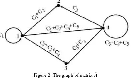
The next step to find the oscillation periodic duration of the system by calculating the eigen value of the matrix
Ã. The graph of the matrix à is shown in Figure 2, From Figure 2, we get the eigenvalue as follows:
ma ma .
This result shows that the oscillation periodic duration of the system depends on 1 and 3,4, 5.We noted that 1 > 3 so the predator has enough time to eat the prey. This is relevant with the real life.
Our next step is giving a value to each holding times. Let 1=6, 2=2, 3=4, 4=1 and 5=1
be the holding times of the system. So, the eigen value of the matrix à is given by,
λ = max{ 1, 3+ 4+ 5} = max{6,6} = 6.
This result shows that the oscillation periodic duration of the system is equal to 6. This result must be different if we choose the other different holding times values.
IV.CONCLUSION
In this section we give some notes of discussing especially in predator-prey system modeled by timed Petri net. The modified model given by:
.
Next we transform the model to get a new model that is given by:
where and
Then, we get the eigenvalue of à as follows:
As we knew that the value of λ is the oscillation periodic duration of the system. So we can conclude that this oscillation periodic duration of the system depends on 1 and 3, 4, 5. In order to the predator has enough
time to eat the prey this could be 1 > 3. Let, 1=6, 2=2, 3=4, 4=1 and 5=1 be the holding times of the
timed Petri net. So, we get the eigenvalue of the matrix Ã
as follows:
λ a 1, 3 + 4 + 5} = max{6,6} = 6
According to this result, we conclude that the oscillation periodic duration of the system is equal to 6. This result also shows that the holding time 2 which is corresponding to place in Figure 2 does not play any role in determining the oscillation periodic duration of the system.
For the future work, the discussing can be continued for finding out whether it is possible to construct a timed Petri net which represents the predator-prey system with all of the holding times in each place plays role in determining the oscillation periodic duration of the system such that the model more realistic than the previous one. For more advance studying, the holding times can be determinded as the interval values.
ACKNOWLEDGEMENT
We wish to give our gratitude to Prof. Zvi Retchkimann Konisberg for giving us the information about this project by his papers. We also really appreciate in every email that he sent related to this project.
Figure 1. Timed Petri net model of predator-prey systems Figure 2. The graph of matrix
REFERENCES
[1] I. Necoara, Model predictive control for max-plus-linear and piecewise affine systems, Neteherland, Technise Universiteit Delft, 2006.
[2] Subiono, The existence of eigenvalues for reducible matrices in max-plus algebra, Surabaya, Mathematics Department FMIPA- ITS, 2008.
[3] Subiono, Aljabar max plus dan terapannya. Surabaya, Department of Mathematic, ITS, 2010.
[4] F. Bacelli, G. Cohen, G. Olsder, and J. Quadrat, Synchronization and Linearty, An algebra for discrete event system, Web Ed, 2001. [5] Z. Retchkiman, “A Mixed lyapunov-max-plus algebra approach to
the stability problem for a two species
ecosystem modeled with timed petri nets,” International Mathematical Forums, vol. 5, pp. 1393-1408, 2010.
[6] Subiono and J. V. D. Woude, “Power algorithms for (Max,+)- and bipartite (Min, Max,+)-systems”, Discrete Event Dynamic Systems: Theory and Applications, vol. 10, no. 4, pp, :369-389, 2000.
[7] Subiono and N. Sofiyana, “Using max-plus algebra in the flow shop scheduling”, IPTEK, The Journal for Technology and Science, vol. 20, 2009, pp. 83-87.
[8] D. Adzkiya, “Membangun model petri net lampu lalu lintas dan simulasinya,” Tesis M.Si., Institut Teknologi Sepuluh Nopember, Surabaya, Indonesia, 2008.