HOW DOES PARENTAL INCOME
AFFECT CHILD LABOR SUPPLY?
EVIDENCE FROM
THE INDONESIA FAMILY LIFE SURVEY
WORKING
PAPER 2 - 2018
February 2018
Elan Satriawan
HOW DOES PARENTAL INCOME
AFFECT CHILD LABOR SUPPLY?
EVIDENCE FROM THE INDONESIA FAMILY LIFE SURVEY
The TNP2K Working Paper Series disseminates the findings of work in progress to encourage discussion and exchange of ideas on poverty, social protection and development issues.
Support to this publication is provided by the Australian Government through the MAHKOTA Program.
The findings, interpretations and conclusions herein are those of the author(s) and do not necessarily reflect the views of the Government of Indonesia or the Government of Australia.
You are free to copy, distribute and transmit this work, for non-commercial purposes.
Suggested citation: Satriawan, E., Ghifari, A.T. 2018. How Does Parental Income Affect Child Labor Supply? Evidence From The Indonesia Family Life Survey. TNP2K Working Paper 2-2018. Jakarta, Indonesia.
To request copies of this paper or for more information, please contact: info@tnp2k.go.id. The papers are also available at the TNP2K (www.tnp2k.go.id).
TNP2K
Grand Kebon Sirih Lt. 4,
Jl. Kebon Sirih Raya No.35, Jakarta Pusat, 10110
TNP2K WORKING PAPER 2 - 2018
February 2018
Elan Satriawan
HOW DOES PARENTAL INCOME AFFECT CHILD LABOR SUPPLY?
EVIDENCE FROM THE INDONESIA FAMILY LIFE SURVEY
Elan Satriawan♦♣and Alif Timur Ghifari♠
Abstract
Drawing on the substitution axiom formulated by Basu and Van (1998) this study examines
the nature of relationship between parental income and child labor supply in Indonesia. To
estimate such relationship, we are benefited by panel data from the last two waves of
Indonesia Family Life Survey (2007 and 2014). We tackle the potential endogeneity in
parental income by controlling for parental fixed-effect. Results shows that parental income
matter to child labor supply. The effect of father’s income looks more significant to all sample
particularly to girls. In rural areas, both parental income matter to girls, and not to boys. The
relationship between a father’s income (and mother’s in rural) with children’s labor hours are
complementary at low level of income, and as income rises, the increments in child labor
hours decreases and at high levels of income, the relationship transforms into a substitute
relationship –resembling an inverted-U shape.
Keywords: Child Labor, Parental Income, IFLS, Indonesia
JEL Classification: J13, O15, J22
♦National Team for Acceleration of Poverty Reduction (TNP2K), Office of Vice President-Republic of Indonesia (email: elan.satriawan@tnp2.go.id)
♣Fakultas Ekonomi & Bisnis, Universitas Gadjah Mada, Jl Sosio-Humaniora No. 1, Bulaksumur Sleman, Yogyakarta 55283, INDONESIA (email: esatriawan@ugm.ac.id)
Table of Contents
1. Introduction 2. Literature Survey
Economic Theory on Child Labor
Empirical Studies on the Substitution Axiom Child Labor Phenomenon in Indonesia 3. Empirical Strategy
4. Data and Principal Features 5. Findings and Discussions
Figure 1. Father’s Income and Child Labor Supply Figure 2. Mother’s Income and Child Labor Supply
11
Table 1. Child Labor Participation Rates in Indonesia Table 2. Descriptive Statistics
Table 3. Effects of Parental Income on Child Labor Hours (Full Sample) Table 4. Effects of Parental Income on Child Labor Hours: Boys vs Girls Table 5. Effects of Parental Income on Child Labor Hours: Urban vs Rural
23 24 25 26 Appendices
1. Introduction
In recent years, the phenomenon of child labor is almost exclusively associated with
developing countries (Ray, 2000). ILO estimates show that 78 million child laborers -the
biggest amount of child laborers in the world- are located in Asia and the Pacific (ILO, 2013).
In Indonesia, a 2012 report by Understanding Children’s Work estimated that about 2.3
million Indonesians aged 7-14 years, or about 7 percent of total children in this age group
were classified as child laborers. When the age group is relaxed, over four million children
aged 5-17 were working as child laborers in Indonesia.
These numbers are disturbingly high in light of the negative educational and human
capital implications associated with child labor. Psacharopoulos (1997) and Beegle et al.
(2008) found that child labor engagement leads to less schooling on average as well as
decreased labor productivity, while Beegle et al. (2004) and Boozer and Suri (2001) found
negative correlation between child labor and educational outcomes in Vietnam and Ghana
respectively. It is also reported that around 87 percent of child laborers in Indonesia are still
enrolled in school and those who mix school with work tend to trail behind those who do not
in terms of school attendance rate by as much as nine percentage points (Understanding
Children’s Work, 2012). Child labor engagement were also found to hamper the development
of children’s mathematical and reading skills (Akabayashi and Psacharopoulos, 1999; Heady,
2003; Sim et al., 2012). Perhaps the worst of all are the findings by Emerson and Souza (2003)
which suggested that intergenerational persistence in child labor exists, meaning that children
of former child laborers have a higher risk of engaging in child labor activities themselves.
Literatures on child labor frequently delve into the determinants of child labor, which
ranged from poverty (Basu and Van, 1998; Swinnerton and Rogers, 1999), credit market
imperfections (Baland and Robinson, 2000), labor market imperfections (Bhalotra and Heady,
2003), poor institutions (Edmonds and Pavcnik, 2005), household size and composition
(Grootaert and Kanbur, 1995; Emerson and Souza, 2007) as well as social norms and
dynasties (Wahba, 2005; Behrman, 1997). However, there is an understanding that present
empirical literature on child labor determinants is relatively young (Basu and Tzannatos,
Against this backdrop, studies done by Ray (2000a, 2000b, 2003) and Amin et al.
(2006) –based on the substitution axiom posited by Basu and Van (1998)1—shows that with regards to child labor, parental income plays a significant role in the household labor supply
decision. The nature of the relationship between parental income and child labor supply is
deemed complementary when child labor hours increases in response to an increase in
parental income. However, an inverse relationship implies that parental income and child
labor supply are substitutes. Understanding the nature of the relationship between parental
income and child labor contains important policy implications. As Amin et al. (2006) notes:
“if children work because a parent cannot work and the family is thus in a state of poverty
then policies to lessen child labor must recognize the need for economic assistance. If children
engage in market work because they accompany a parent to work based on social and cultural
mores, then policies to lessen children's market work and increase children's schooling must
accommodate the cultural climate”.
In the context of parental income as child labor determinants, the existing body of
literature in various countries report mixed results between countries, and even within
countries, studies have found that the gender of parents also influences whether parental
income (or other household wealth measures) and child labor are substitutes or complements
[Ray (2000a, 2000b, 2003); Amin et al (2006); Basu et al (2010)]. This emphasizes the fact
that while child labor might be an international issue, there are characteristics of child labor
unique to each country. In light of the relatively significant amount of child laborers in
Indonesia as well as the negative impacts of child labor, understanding the relationship
between child labor and parental income in Indonesia becomes crucial. Literatures on child
labor using Indonesian data is rather limited when compared to Latin American data or
African data and, to the best of the authors’ knowledge, no research have ever been undertaken
to see whether parental income and child labor supply are substitutes or complements in
Indonesia.
To that aim, this study benefits from the use of panel data from the last two waves
(2007 and 2014) of the Indonesian Family Life Survey (IFLS), a longitudinal data set
containing rich socioeconomic information on both individuals and households in Indonesia.
1 Basu and Van (1998) presented a framework of child labor containing two fundamental axioms, the luxury
We exploit the data’s panel characteristics to handle potential endogeneity of parental income
due to presence of unobserved heterogeneity. Particularly, we include in the empirical model
parental fixed-effects to control for time-invariant unobserved parental preference that may
lead to biased parameters.
This study found that in Indonesia, father and child labor are complementary at lower
level of wages particularly for girls and for rural sample. However, at higher level of wages,
the relationship transforms into a substitute relationship. This implies two things: first, when
fathers are working for low wages, the household faces capital constraint. Children are then
forced to work to help the household meet their subsequent needs, in line with Basu and Van’s
luxury axiom. Second, when a father’s wage is relatively high enough, the household is then
assumed to have enough financial security and thus the children do not have to work. This
shows that the relationship between child labor hours and father’s income resembles an
inverted U-shape.
The structure of this paper is as follows. Next section surveys child labor literature
including both theory and empirical work. After that, in section 3, we set up the empirical
strategy in which we specify our empirical model to estimate how parental income affects
child labor and discuss the estimation issues. Then, in section 4, we discuss the data and
variable measurement. The results and discussion of the findings are presented in section 5.
Finally, section 6 concludes and provides policy recommendations.
2. Literature Survey
Economic Theory on Child Labor
When analyzing the phenomenon of child labor, it is imperative to recognize child
labor engagement as part of the household labor decision. The seminal work of Becker (1965)
on the allocation of time and its many extensions on household behavior helps explain how
households allocate their labor hours and provides the theoretical foundation on child labor
decisions. In Becker’s model, households jointly make decisions on a myriad of issues to
satisfy a “common set” of family preferences, including the number of children in a household
as well as how to allocate the time of household members between work, schooling, leisure,
and household production.
Recognizing that the decision to engage in child labor is made by the household, it is
between parent and child. Basu and Van (1998) posits two crucial assumptions, or axioms,
that underlie the theory as well as much of the existing literature on child labor. The first
assumption suggests that when adults work full time, children are sent to work only if income
levels of the household are less than subsistence consumption.2This assumption is known as the luxury axiom.
The second assumption, also known as the substitution axiom suggests that child and
adult labor are interchangeable from a firm’s perspective, subject to an equivalency
correction. This means that from a technical point of view, adult labor can be substituted with
child labor, that is, children can do some, if not all jobs that are usually thought to be reserved
for adults. Both axioms implicitly support the notion that households are altruistic in a sense
that they prefer children not to engage in labor activities unless forced to by circumstances.
Empirical Studies on the Substitution Axiom
Substantial researches have contributed findings to support the luxury axiom, most
notably Basu and Tzannatos (2003), Delap (2001), Grootaert (1999), Ravallion and Woodon
(2000), and Ray (2000a, 2000b). However, contemporary empirical researches testing the
substitution axioms were relatively scarcer, with mixed results.
Ray (2000a, 2000b) was the first to econometrically test the substitution axioms, using
data on child labor from Pakistan and Peru to do so. He found that parental income and child
labor were negatively correlated in Peru, indicating that parents and children were substitutes,
while in Pakistan, mother’s wages and child labor were positively correlated, indicating a
complementary relationship. The difference in relationship between parental income and child
labor in Peru and Pakistan led Ray (2003) to test the relationship once again in Ghana. The
paper found that in Ghanaian rural areas, at low level of wages male and female labor were
complementary with child labor while at high level of wages child labor and female labor
were substitutes. The study notes that the results between rural and urban areas differ greatly,
suggesting that child labor in rural and urban areas were affected by different factors.
Basu et al (2010), using household surveys in two mid-Himalayan regions in India
(Himachal Pradesh and Uttaranchal), test the inverted-U relationship hypotheses between
inherited land owned by household and child labor. Controlling for both child and household
characteristics and including village fixed effects they find size of inherited land correlates
positively with child labor but with decreasing return supporting the inverted-U hypotheses.
In Bangladesh, Amin et al. (2006) estimated the relationship between parental income
and child labor in eight different demographic groups. The paper reported mixed results.
Father and children were substitutes in the household labor supply decision for younger rural
boys and girls as well as younger urban boys, but father and older rural boys were
complements. Meanwhile, mother and children were found to be complements in seven out
of the eight demographic groups. This can be attributed to the social customs in Bangladesh
that encourages boys to be kept busy in order to stay out of trouble and that pressures girls to
not be left home alone if her mother is working outside the house. They also found that
parental income had little effect on children’s household work.
Using data from Egypt, Diamond and Fayed (1998) simulated employment effects on
child labor. Their findings reported that adult males tend to be complements of child labor,
while adult females were substitutes. This finding reinforces the result of the study carried out
by Grant and Hamermesh (1981) which found that white women and youths were substitutes
in production in the USA.
Child Labor Phenomenon in Indonesia
The Government of Indonesia has tried to combat child labor through a series of policy
regulations such as Law No. 20/1999 on the Ratification of ILO Convention 138 as well as
Law No. 13/2003 (also known as the Manpower Act) that limits the age of workers and the
types of jobs allowed for children. However, as Grootaert and Kanbur (1995) notes, simply
restricting some forms of child labor, or even banning it entirely might be ineffective and in
some cases, counterproductive. Knight (1980) suggests that a child labor ban might be
detrimental in a sense that when child labor is prohibited by law, the law is then powerless to
introduce measures to protect child laborers since they are not recognized by the law.
Moehling (1999) also found that the minimum age limit on child work has had relatively little
effect on the long run decline of child labor. Therefore, instead of a straightforward ban on
child labor more effective policies are needed to address child labor issues. To be effective,
these policies must take into account the determinants and nature of child labor. To help
contextualize the issue, below we provide a brief discussion on the nature of child labor in
As of 2009, over 2.3 million children aged 7-14 worked as child laborers in Indonesia,
with 2 million located in rural areas while the rest originated from urban areas (Understanding
Children Work, 2012). Children working in urban areas can be found in the streets selling
newspaper, candies, and drinks or singing and begging for money at traffic lights or buses
(Priyambada et al. 2005) while in rural areas children were found working in the fields or
tending to livestock. When disaggregated by sectors, the agricultural sector accounts for the
largest share of child labor in Indonesia, with 58 percent of working children aged 7-14
employed there. The services sector, which employs 27 percent of all child laborers, is second
while manufacturing with 7 percent comes a distant third (Understanding Children’s Work,
2012). The report goes on to highlight the fact that one third of the children in the services
sector work in domestic services, which is a particular policy concern as their work is then
not observable and they might therefore be vulnerable to overexploitation.
Gender was found to influence the type of work that children does. Boys tend to work
in the agriculture sector, while girls were more likely to work in services and manufacturing.
Age, unsurprisingly, also affects the type of jobs children engages in, as younger children
were more likely to work in agriculture and older children were more likely to be found
working in the manufacturing and services sector. Finally, geographical location also plays a
part. Children in rural areas tend to work in agriculture, and their urban counterpart were more
likely to work in the manufacturing and services sector.
While prevalence of child labor in Indonesia is relatively lower than other developing
countries, in absolute terms it continues to be a significant concern (Understanding Children
Work, 2012). Notwithstanding the recent influx of literature on child labor in Indonesia as
studies endeavored to find the determinants of child labor (Chang, 2006; Kis-Katos and
Schulze, 2011), it must be noted that studies on the relationship between parental income and
child labor in Indonesia are conspicuous by its absence. Chang (2006), which estimated the
roles of family affluence, bargaining power, and parental educational attainments on child
labor status using IFLS2 and IFLS3 did control for the effect of family income on child labor
status. However, the study used per capita expenditure to proxy for household income rather
than parental income and disregarded the difference in nature between a father’s income and
a mother’s income with respect to child labor status. We argue that the difference between the
effect of father’s income and mother’s income on child labor is vital for policy formulation.
specific individuals (fathers or mothers) in order to decrease child labor, for instance by
holding job training programs for individuals with children in order to increase their income.
More generally, the government will then be able to optimally formulate new policies, or
reform existing policies, on child labor.
In the reminder of this analysis, we will therefore focus on the difference between
father’s income and a mother’s income in determining the level of child labor engagement in
the household.
3. Empirical Strategy
We formulate empirical specification to examine the relationship between parental
income and child labor. Particularly we test whether the relationship support substitution
axiom. To do so, we borrow empirical models by Ray (2000a, 2000b, 2003) and Amin et al.
(2006). We start with basic empirical model as follows:
𝑐𝑐𝑐𝑐𝑐𝑐𝑐𝑐𝑖𝑖𝑖𝑖ℎ𝑡𝑡𝑡𝑡 = 𝛼𝛼𝛼𝛼+𝛽𝛽𝛽𝛽1𝑓𝑓𝑓𝑓𝑓𝑓𝑓𝑓𝑓𝑓𝑓𝑓𝑐𝑐𝑐𝑐ℎ𝑡𝑡𝑡𝑡+𝛽𝛽𝛽𝛽2𝑚𝑚𝑚𝑚𝑓𝑓𝑓𝑓𝑓𝑓𝑓𝑓𝑐𝑐𝑐𝑐ℎ𝑡𝑡𝑡𝑡+𝑿𝑿𝑿𝑿𝒊𝒊𝒊𝒊𝒊𝒊𝒊𝒊′ 𝜸𝜸𝜸𝜸+𝑯𝑯𝑯𝑯𝑯𝑯𝑯𝑯𝒉𝒉𝒉𝒉𝒊𝒊𝒊𝒊′ 𝜽𝜽𝜽𝜽+𝜀𝜀𝜀𝜀𝑖𝑖𝑖𝑖𝑡𝑡𝑡𝑡
where 𝑐𝑐𝑐𝑐𝑐𝑐𝑐𝑐𝑖𝑖𝑖𝑖ℎ𝑡𝑡𝑡𝑡 measures child labor,𝑓𝑓𝑓𝑓𝑓𝑓𝑓𝑓𝑓𝑓𝑓𝑓𝑐𝑐𝑐𝑐𝑖𝑖𝑖𝑖ℎ𝑡𝑡𝑡𝑡 and 𝑚𝑚𝑚𝑚𝑓𝑓𝑓𝑓𝑓𝑓𝑓𝑓𝑐𝑐𝑐𝑐𝑖𝑖𝑖𝑖ℎ𝑡𝑡𝑡𝑡are respectively father’s and mother’s income, 𝑿𝑿𝑿𝑿𝒊𝒊𝒊𝒊𝒊𝒊𝒊𝒊′ and 𝑯𝑯𝑯𝑯𝑯𝑯𝑯𝑯𝒉𝒉𝒉𝒉𝒊𝒊𝒊𝒊′ are respectively vector of individual child and household characteristics, and 𝜀𝜀𝜀𝜀𝑖𝑖𝑖𝑖𝑡𝑡𝑡𝑡 denotes error term. Subscripts iht are respectively denote for child labor iin household hand period t.
The parental income of child i are differentiated into father’s income and mother’s
income in the regression function to account for the difference in nature between father and
mother’s income towards child labor engagement. The practice of differentiating parental
income by gender has been used before, notably by both Ray (2000a, 2000b, 2003) as well as
Amin et al. (2006) and can be traced back to Grant and Hamermesh (1981).
Estimating effect of parental income on child labor supply with Ordinary Least
Squares – ignoring correlation between parental income and error term—will lead to biased
parameters. We thus control for parental fixed effect to eliminate potential bias, as households
engaging in child labor may systematically differ from household that do not. For instance,
households/parents might have a fixed preference or motivation in sending children to work.
As an added measure, reflecting on the fact that some of the children in the sample are
members of the same household, the standard errors of the coefficients have also been
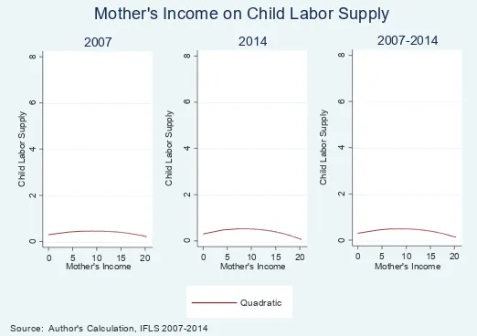
Motivating by the relation between child labor supply and parental income as depicted
in Figures 1 and 2, we include quadratic form of parental income (𝑓𝑓𝑓𝑓𝑓𝑓𝑓𝑓𝑓𝑓𝑓𝑓𝑐𝑐𝑐𝑐ℎ𝑡𝑡𝑡𝑡2 and 𝑚𝑚𝑚𝑚𝑓𝑓𝑓𝑓𝑓𝑓𝑓𝑓𝑐𝑐𝑐𝑐ℎ𝑡𝑡𝑡𝑡2 ) to capture the decreasing or increasing marginal effects of parental income. A year dummy
(yr14) and district dummy are included to control for difference in ‘child labor market’ across
observation periods and districts respectively. Our expanded empirical model is then:
𝑐𝑐𝑐𝑐𝑐𝑐𝑐𝑐𝑖𝑖𝑖𝑖ℎ𝑡𝑡𝑡𝑡 =𝛽𝛽𝛽𝛽0+𝛿𝛿𝛿𝛿0𝑦𝑦𝑦𝑦𝑦𝑦𝑦𝑦14𝑡𝑡𝑡𝑡+𝛽𝛽𝛽𝛽1𝑓𝑓𝑓𝑓𝑓𝑓𝑓𝑓𝑓𝑓𝑓𝑓𝑐𝑐𝑐𝑐ℎ𝑡𝑡𝑡𝑡+𝛽𝛽𝛽𝛽2𝑓𝑓𝑓𝑓𝑓𝑓𝑓𝑓𝑓𝑓𝑓𝑓𝑐𝑐𝑐𝑐ℎ𝑡𝑡𝑡𝑡2 +𝛽𝛽𝛽𝛽3𝑚𝑚𝑚𝑚𝑓𝑓𝑓𝑓𝑓𝑓𝑓𝑓𝑐𝑐𝑐𝑐ℎ𝑡𝑡𝑡𝑡+𝛽𝛽𝛽𝛽4𝑚𝑚𝑚𝑚𝑓𝑓𝑓𝑓𝑓𝑓𝑓𝑓𝑐𝑐𝑐𝑐ℎ𝑡𝑡𝑡𝑡2 +𝑿𝑿𝑿𝑿𝒊𝒊𝒊𝒊𝒊𝒊𝒊𝒊′ 𝜸𝜸𝜸𝜸+𝑯𝑯𝑯𝑯𝑯𝑯𝑯𝑯𝒉𝒉𝒉𝒉𝒊𝒊𝒊𝒊′ 𝜽𝜽𝜽𝜽
+𝝁𝝁𝝁𝝁𝒉𝒉𝒉𝒉 +𝝅𝝅𝝅𝝅𝒅𝒅𝒅𝒅+𝜀𝜀𝜀𝜀𝑖𝑖𝑖𝑖𝑡𝑡𝑡𝑡
Figure 1. Father’s Income and Child Labor Supply
Figure 2. Mother’s Income and Child Labor Supply
-2
Source: Author's Calculation, IFLS 2007-2014
Father's Income on Child Labor Supply
Quadratic
Source: Author's Calculation, IFLS 2007-2014
Mother's Income on Child Labor Supply
Our main parameters of interest are thus β1,β2,β3 and β1. After controlling for both
observed covariates and time-invariant unobserved heterogeneity, we argue that the
parameters of interest are unbiased. If both β1 and β2 (β3 and β4) are significant, father’s
(mother’s income) should affect child labor supply in quadratic relationship –either exhibiting
positive or negative effects with diminishing return. Some conditions however may invalidate
our identification assumption. For example, if parental preference or motivation are not fixed
across observation period perhaps due to economic shock, our parameters of interest may
accordingly not unbiased.
We run the model on three samples; the full sample and two disaggregated sample: by
residential location as well as by gender type. The reasoning behind this is that location of
residence and gender type is an important determinant of child labor in Indonesia
(Understanding Children’s Work, 2012), thus, samples are disaggregated to help better
understand child labor phenomenon in Indonesia and isolate area-specific or gender-specific
characteristics of child labor.
4. Data and Principal Features
This study uses data from the Indonesian Family Life Survey.3The Indonesian Family Life Survey is a continuing longitudinal socioeconomic and health survey based on a sample
of households representing about 83% of the Indonesian population. The IFLS collects a
wealth of data on individual respondents, their families and households, the communities in
which they live, as well as the health and education facilities they use. The IFLS has been
administered 5 times, from 1993 to 2015. The first wave (IFLS1) was carried out in 1993 and
covered individuals living in 7,224 households. The second wave (IFLS2) covered the same
individuals in 1997 while IFLS2+ measured the impact of the Indonesian crisis in 1998. The
third wave (IFLS3) was administered in 2000 with the same respondents, and the fourth wave
(IFLS4) was fielded in late 2007-early 2008. Meanwhile, the fifth wave (IFLS5) consisted of
the 1993 households and their split-offs and was fielded in late 2014 and early 2015, which
covered 50,148 individuals living in 16,204 households.
Due to the structure and evolving nature of the IFLS questionnaires, questions on child
labor incidence are only present from the third wave of the study. As this study is interested
in analyzing the recent trend of child labor engagement, this paper only focuses on data from
the last two waves. Data on child labor incidence can be retrieved from Book 5, where IFLS4
contains information on 8,505 children while the IFLS5 data set covered 10,381 children aged
5-14. However, this study limits itself to analyzing data of children aged 10-14. The reason
for this limitation is that the incidence of child labor in the IFLS data is concentrated on
children aged 10-14. As this paper is interested in analyzing the relationship between the
phenomenon of child labor and parental income, the focus of the analysis is on the age group
where children are more likely to work. The final dataset consists of 8,475 individuals from
5,327 households across the two waves.
This study uses child labor hours as the dependent variable rather than a dummy
variable indicating whether child iis engaged in child labor activities or not. The reason for
this is because child labor hours is deemed as a crucial measure of child welfare, and more
importantly, it is also an essential component in evaluating the cost of work in terms of health
and human capital accumulation (Rosati and Rossi, 2003)
Child labor hours is determined by looking at answers to two questions. The first
question inquired as to whether the child worked last week. If the child (or her parents)
confirms that she has been working last week, the respondents are then asked about the
number of hours she spent working last week. If the child confirms that she did not work last
week, then her labor hours is set to zero. Monthly child labor hours is then estimated by
multiplying weekly labor hours by 4.
In the IFLS questionnaires, child laborers are divided into two types, those working
for wages and those working for family business. Nonetheless, based on the findings of Sim
et al. (2012), the negative effect of child labor in Indonesia affects those who work within the
family as well as those who works outside it. This might be explained by the fact that
hazardous work conditions were common for both children engaged in family business or
working for wages (Understanding Children’s Work, 2012). Therefore, this study does not
differentiate between those two types of work in defining child labor.
On the subject of parental characteristics, namely parental education and income, one
particular caveat should be noted. As some missing data were observed in the data set,
imputations were made to correct for missing values and data imperfection. Appendix 1
5. Findings and Discussions
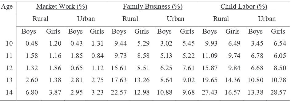
Table 1 presents child labor participation rates in Indonesia as well as the breakdown
of child labor incidence based on types and genders. In general, child labor is more prevalent
in rural areas than in urban areas for all age group, while higher age is associated with an
increase in child labor incidence. The increase in child labor engagement with age might be
explained by rising productivity, which in turn leads to rising opportunity cost of keeping
children in school. There is also suggestion that the lack of access to post-primary schooling,
especially in rural areas decreases the opportunity cost of child labor (Understanding
Children’s Work, 2012). The data shows that the amount of child laborers in rural areas is
a cause for concern, with more than one quarter of 14-year-old boys found working as child
laborers.
Table 1. Child Labor Participation Rates in Indonesia
Age Market Work (%) Family Business (%) Child Labor (%)
Rural Urban Rural Urban Rural Urban
Boys Girls Boys Girls Boys Girls Boys Girls Boys Girls Boys Girls
10 0.48 1.20 0.43 1.31 9.44 5.29 3.02 5.45 9.93 6.49 3.45 6.54
11 1.58 1.16 1.85 0.84 9.73 8.58 5.13 5.22 11.09 9.74 6.78 6.05
12 1.32 1.86 0.65 1.12 15.61 8.51 6.25 7.61 15.87 9.84 6.68 8.50
13 2.60 1.38 2.81 2.75 17.63 13.26 8.64 9.02 19.65 14.36 10.80 10.78
14 6.80 3.87 2.95 3.23 22.57 12.98 10.88 9.68 27.43 16.57 13.38 28.57
Source: Author’s analyses based on IFLS4 (2007) and IFLS5 (2014)
Popular illustrations on child labor usually paints a picture of children working in
dimly lit factories or forced into slavery or prostitution. However, Edmonds (2008) argues
that those cases represents extreme examples of child labor and are not widespread. In truth
most child laborers around the world work within the household and only a few work outside
the household for pay (Edmonds and Pavcnik, 2005). The IFLS data reflects this fact,
as the majority of child laborers are found to be working for family business.
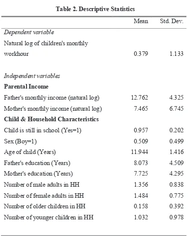
Table 2 displays the mean and standard deviation of parental income and other control
variables. For parental income, it shows that fathers have a higher average income than
mothers implying that in Indonesia households still rely on fathers to act as the main
likely to work full-time than men. In our sample, number of boys and girls were almost
balanced, most children were still in school (95.7%), and average age was almost 12 years
old.
Table 2. Descriptive Statistics
Mean Std. Dev.
Dependent variable
Natural log of children's monthly
workhour 0.379 1.133
Independent variables
Parental Income
Father's monthly income (natural log) 12.762 4.325
Mother's monthly income (natural log) 7.465 6.745
Child & Household Characteristics
Child is still in school (Yes=1) 0.957 0.202
Sex (Boy=1) 0.509 0.499
Age of child (Years) 11.944 1.416
Father's education (Years) 8.073 4.509
Mother's education (Years) 7.725 4.295
Number of male adults in HH 1.356 0.838
Number of female adults in HH 1.484 0.775
Number of older children in HH 0.158 0.392
Number of younger children in HH 1.032 0.978
Source: Authors’ calculation based on IFLS4 (2007) and IFLS5 (2014). N=8,475
We also control for household characteristics including parental education, number of
adult female and male in the household, number of older and younger children in the
household. Mean and standard deviation for each household characteristics can be seen in
Findings
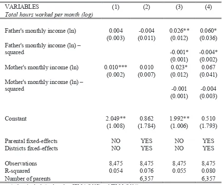
Table 3 presents the results of the regression on the full sample. While this study uses
a quadratic model, a model that assumes linear relationship between parental income and child
labor hours is also displayed in Table 2. This is done to show the contrast in results between
differing models and assumptions. The difference between the first and the second regression
is that the second regression uses household fixed effect to correct for potential biases. Results
from the linear functional relationship between the two (columns 1 and 2) suggest that the
relationship between a mother and her child in the household labor supply is complementary,
with child labor hours increasing as wages increases.
Table 3. Effects of Parental Income on Child Labor Hours (Full Sample)
VARIABLES (1) (2) (3) (4)
Total hours worked per month (log)
Father's monthly income (ln) 0.004 -0.004 0.026** 0.060*
(0.003) (0.011) (0.012) (0.036) Father's monthly income (ln) –
squared -0.001* -0.004*
(0.001) (0.002)
Mother's monthly income (ln) 0.010*** 0.010 0.023* 0.067
(0.002) (0.007) (0.012) (0.041)
Parental fixed-effects NO YES NO YES
Districts fixed-effects NO YES NO YES
Observations 8,475 8,475 8,475 8,475
R-squared 0.054 0.076 0.055 0.080
Number of parents 6,357 6,357
Source: Authors’ calculation based on IFLS4 (2007) and IFLS5 (2014)
In the third and fourth columns, following Ray (2003) and Basu et al (2010) the
relationship between parental incomes and child labor hours is modeled as a quadratic model,
therefore the squared natural log of both parents’ income are included in the regression model.
The results from the quadratic model paints a different light. First, the magnitude of the impact
of an increase in mother’s income towards child labor hours is markedly higher and
significant, but its square form is not significant indicating that mother’s income complements
linearly with working hours of children. Second, modelling the relationship as quadratic
causes the father’s income to become significant. Particularly, at low level of wages, the
relationship between a father and working hours of children is complementary. However, as
wages increases, the increments in child labor hours decreases, and at high level of wages,
father’s income and child labor are substitutes. When controlling for parental and districts
fixed-effect, however, the effect of mother’s income disappears. On the contrary, effect of
father’s income on child’s working hours becomes significant supporting inverted-U form: as
income increases, child working hours increase with decreasing return.
This result would appear to be consistent with the idea of parental altruism in the
substitution hypothesis, in a sense that child labor is deemed undesirable and fathers will
decrease their children’s labor hours as their own income increases. This finding is also in
line with Ray (2003) which reported that parents in Ghana behaved similarly when income
increases.
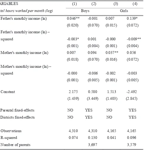
Tables 4 and 5 presents the regression results when samples are disaggregated by
gender and region types respectively. Results in Table 4 show that the quadratic relationship
between parental income and child’s working hours in full sample in Table 3 is explained
mainly by the quadratic relationship between father’s income and girl’s working hours –the
effect to boy’s working hours become shrink and insignificant. This is notable, as Parish and
Willis (1993) suggest that compared to their male counterpart, girls were more likely to help
the household by working or by bringing other resources into the household. This result
implies that when households are facing capital constraints, girls are first in line to work and
Table 4. Effects of Parental Income on Child Labor Hours: Boys vs Girls
VARIABLES (1) (2) (3) (4)
Total hours worked per month (log) Boys Girls
Father's monthly income (ln) 0.046** -0.001 0.007 0.139*
(0.020) (0.070) (0.015) (0.072)
Father's monthly income (ln) –
squared -0.003* 0.001 -0.000 -0.009**
(0.001) (0.004) (0.001) (0.004)
Mother's monthly income (ln) 0.007 0.094 0.037** 0.056
(0.018) (0.070) (0.016) (0.072)
Mother's monthly income (ln) –
squared -0.000 -0.006 -0.002 -0.003
(0.001) (0.005) (0.001) (0.005)
Constant 2.175 0.580 1.513 -2.492
(1.439) (3.449) (1.403) (2.845)
Parental fixed-effects NO YES NO YES
Districts fixed-effects NO YES NO YES
Observations 4,310 4,310 4,165 4,165
R-squared 0.074 0.130 0.041 0.096
Number of parents 3,697 3,579
Source: Author’s analyses based on IFLS4 (2007) and IFLS5 (2014)
Note: ***, **, and * denotes significance at the 1, 5, and 10 percent level respectively. Regression
were done with a full set of control variables that includes age, age squared, school enrollment,
number of younger and older children in the household, years of schooling parent, the number of
male and female adults in the household, and a year dummy. A complete table can be found in the
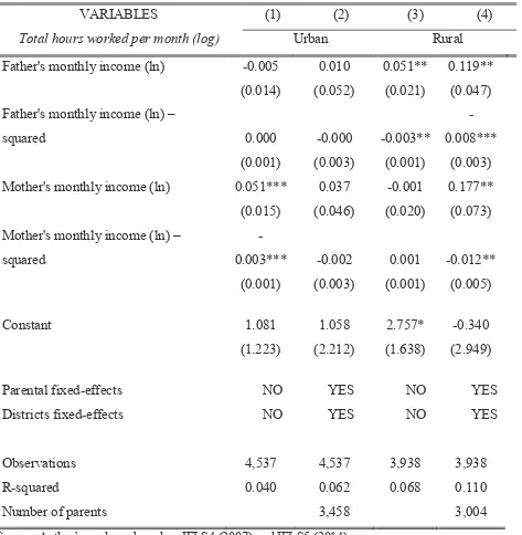
Table 5. Effects of Parental Income on Child Labor Hours: Urban vs Rural
VARIABLES (1) (2) (3) (4)
Total hours worked per month (log) Urban Rural
Father's monthly income (ln) -0.005 0.010 0.051** 0.119**
(0.014) (0.052) (0.021) (0.047)
Father's monthly income (ln) –
squared 0.000 -0.000 -0.003**
-0.008***
(0.001) (0.003) (0.001) (0.003)
Mother's monthly income (ln) 0.051*** 0.037 -0.001 0.177**
(0.015) (0.046) (0.020) (0.073)
Mother's monthly income (ln) –
squared
-0.003*** -0.002 0.001 -0.012**
(0.001) (0.003) (0.001) (0.005)
Constant 1.081 1.058 2.757* -0.340
(1.223) (2.212) (1.638) (2.949)
Parental fixed-effects NO YES NO YES
Districts fixed-effects NO YES NO YES
Observations 4,537 4,537 3,938 3,938
R-squared 0.040 0.062 0.068 0.110
Number of parents 3,458 3,004
Source: Author’s analyses based on IFLS4 (2007) and IFLS5 (2014)
Note: ***, **, and * denotes significance at the 1, 5, and 10 percent level respectively. Regression
were done with a full set of control variables that includes age, age squared, school enrollment, number
of younger and older children in the household, years of schooling parent, the number of male and
female adults in the household, and a year dummy. A complete table can be found in the appendix.
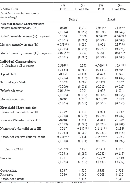
Results from Table 5 suggests that quadratic relationship between father’s income and
child’s working hours persists strong and significant in rural areas. This result complements
the findings of Amin et al. (2006), which found a substitute relationship between the father
and children in a rural setting. In addition, when disaggregating by urban-rural, we find also
such relationship between mother’s income and child’s working hours. Interestingly, the
magnitude of mother’s income effects is greater than those of father’s income. This finding is
consistent with the findings of Ray (2003), and suggest that when mothers are forced to work
for low wages in rural areas, this might be an indication that the household is facing severe
financial constraints and therefore requires additional income in the form of child work.
From the remaining control variables on individual and household characteristics,
there are a couple of points to note. First, unlike previous studies, age is not found to be
significant, both in the full sample and in the disaggregated ones. This suggest that parental
income, rather than age, plays a significant role in determining child labor outcomes in
Indonesia.
Second, being enrolled in school also has a large negative effect on estimated child
labor hours. This suggests that across all samples, a child who is enrolled in school is less
likely to engage in child labor activities compared to a child who dropped out of school.
Understanding Children’s Work (2012) highlighted the fact that almost two thirds of children
in Indonesia not currently engaged in schooling were found to be working, while Ravallion
and Woodon (2000) also noted some substitutability between child labor and school
enrollment. This implies that one of the most straightforward methods on decreasing child
labor incidence in Indonesia is through policies that ensures all children are enrolled in school.
Third, parental education initially appears to be important determinant that lower child
labor. However, after controlling for household/parental fixed-effects, the significant effects
disappear. There are a couple of reasons for this. This might imply that there are other
unobserved household/parental heterogeneity matter more in reducing child labor. It might
however also be the case that because parental education rarely changes between waves, when
using FE method this means that we rarely see significant coefficients.
Fourth, we also find that having a sibling in the household decreases estimated child
labor hours, which may indicate that the burden of working is likely to be shared between
children. When comparing between older and younger siblings, while the effect of both on
child labor hours than the presence of a younger sibling. A striking discovery regarding older
siblings is that when sample is further disaggregated by gender, having an older sibling in the
household is beneficial for boys only, while girls are seemingly unaffected. This suggest that
when the household has an additional source of income in the form of an older sibling, parents
prefer to allocate scarce resources, in this case, time spent not working, to male children rather
than female children. This result is also somewhat reflected in Edmonds (2006), which found
that the time a child spent working increases when younger boys are present in the household.
6. Conclusions and Policy Implications
This study examines the relationship between parental income and child labor supply
as well as its subsequent nature in Indonesia, and contributes to the small yet growing
literature on child labor in Indonesia. While previous studies on the relationship between
parental income and child labor mainly used one period data to estimate the relationship, this
study benefits from the panel feature of the Indonesian Family Life Survey, which made it
possible to control for household time-invariant unobserved heterogeneity and address
potential bias from its correlation with parental income. Regressions were carried out over
three types of sample: the full sample, sample disaggregated by gender type, and by type of
region to gain a better understanding of child labor phenomenon in Indonesia and isolate
location-specific or gender-specific factors.
This study found that in Indonesia, father and child labor are complementary at lower
level of wages in all of samples except for urban and boys only samples. However, at higher
level of wages, the relationship transforms into a substitute relationship. This implies two
things: first, when fathers are working for low wages, the household faces capital constraint.
Children are then forced to work to help the household meet their subsequent needs, in line
with Basu and Van’s luxury axiom where children work only if the income of the household
are less than subsistence consumption. Second, when a father’s wage is relatively high
enough, the household is then assumed to have enough financial security and thus the children
do not have to work. This shows that the relationship between child labor hours and father’s
income resembles an inverted U-shape. This result further reinforces the findings of Ray
(2003) and suggests that parental altruism exists with regards to child labor, that is, parents
do not let their children work if the family has enough income. For mothers, income and child
There is no silver bullet when it comes to tackle the child labor problem in a sense that
rather than just one policy or measure, a combination of policies and effective law
implementation are crucially needed to successfully combat the problem. Policies that aim at
banning child labor indiscriminately without addressing the root cause of child labor would
help neither the children nor household, especially when the household is facing poverty
(Amin et al, 2006). Findings on the unique relationship between mother and children in the
household labor supply decision suggest that policies to lessen child labor should focus on
improving mother’s welfare, chiefly mothers who works for low wages. The improvement in
mother’s welfare should benefit their children, especially girls, and decrease child labor hours.
A noteworthy method proposed by Amin et al. (2006) to decrease child labor is by
increasing access to credit. As shown by Wahid (1999), the presence of microcredit helps
increase employment opportunities for women and alleviate poverty in Bangladesh. Widening
access to existing labor markets is another avenue to consider, and should also help increase
welfare. Finally, social protection programs that targets women and children in Indonesia,
such as the Conditional Cash Transfer (Program Keluarga Harapan/PKH) and Education
Assistance (Program Indonesia Pintar/PIP) should also be strengthened by incorporating
mechanisms to help deal with child labor issues. As shown by Skoufias and Parker (2001) in
Mexico and de Hoop and Rosati (2013) more generally, while cash transfer programs are not
usually designed to target child labor, those programs are generally effective in reducing child
References
Akabayashi, H. and G. Psacharopoulos (1999), "The Trade-off between Child Labour and Human Capital Formation: A Tanzanian Case Study", Journal of Development Studies 35: 120-140.
Amin, S., S. Quayes, and J. M. Rives. (2006). Are Children and Parents Substitutes or Complements in the Family Labor Supply Decision in Bangladesh? The Journal of Developing Areas,40(1), 15–37.
Baland, J. and J. A. Robinson (2000), “Is Child Labor Inefficient?”, Journal of Political Economy 108: 663-679.
Basu, K. and P. H. Van (1998), “The Economics of Child Labor”, The American Economic Review, Vol 88, pp. 413-427.
Basu, K. and Z. Tzannatos (2003), “The Global Child Labor Problem: What Do We Know and What Can We Do?” The World Bank Economic Review, Vol. 17, No.2, pp.147-173.
Basu, K., S. Das, and B. Dhutta (2010), “Child Labor and Household Wealth: Theory and Empirical Evidence on Inverted-U”, Journal of Development Economics, Vol 91/1, pp. 8-14.
Becker, G. (1965), “A Theory of the Allocation of Time”, Economic Journal, Vol. 75, pp. 493-5 17.
Beegle, K., R. Dehejia and R. Gatti, (2004), "Why Should We Care About Child Labor? The Education, Labor Market, and Health Consequences of Child Labor," NBER Working Papers 10980.
Beegle, K., R. Dehejia, R. Gatti and S. Krutikova (2008), “The Consequences of Child Labor: Evidence from Longitudinal Data in Rural Tanzania”, World Bank Working Paper 4677.
Behrman, J. (1997), Women's Schooling and Child Education: A Survey. Mimeo, University of Pennsylvania
Bhalotra, S. and C. Heady (2003), “Child Farm Labor: The Wealth Paradox”, The World Bank Economic Review, Vol. 17, pp. 197-227.
Boozer, M. and T. Suri (2001), “Child Labor and Schooling Decisions in Ghana”, Unpublished paper (Yale University).
Chang, Y. (2006), "Determinants of Child Labour in Indonesia: The Roles of Family Affluence, Bargaining Power and Parents' Educational Attainments", Thesis, Department of Economics, National University of Singapore.
de Hoop, J., & Rosati, F. C. (2014). Cash Transfers and Child Labor. World Bank Research Observer,vol 29(2),pp 202-234.
Delap, E. (2001), “Economic and Cultural Forces in the Child Labour Debate: Evidence from Urban Bangladesh”, Journal of Development Studies, Vol. 37, pp.1-22.
Edmonds, E. (2006), “Understanding sibling differences in child labor”, Journal of Population Economics, Vol 19, pp 795-821.
Edmonds, E. (2008), “Child Labor”, in T. Schultz and J. Strauss (Eds), Handbook of Development Economics Volume IV, Elsevier.
Edmonds, E. and N. Pavcnik (2005), “Child labor in the Global Economy”, Journal of Economic Perspectives, Vol 19, pp 199-220.
Emerson, P. and A. Souza (2003), “Is There a Child Labor Trap? Intergenerational persistence of child labor in Brazil”, Economic Development and Cultural Change Vol 51, pp 375-398.
Emerson, P. and A. Souza (2007), “Child Labor, School Attendance, and Intrahousehold Gender Bias In Brazil”. The World Bank Economic Review, Vol 21(2), pp 301-316.
Government of Indonesia (1999), Act of Republic of Indonesia No. 20 of 1999 on Ratification of ILO Convention 138.
Government of Indonesia (2003), Act of Republic of Indonesia No. 13 of 2003
Grant, J. and D. Hamermesh (1981), Labor Market Competition among Youths, White Women, and Others, Review of Economics and Statistics, Vol. 63, No. 3, pp. 354-60.
Grootaert, C. and R. Kanbur (1995), Child Labour: An Economic Perspective. International Labour Review, 134(2).
ILO (2013), Marking Progress Against Child Labour - Global Estimates and Trends 2000-2012.
Kis-Katos, K. and G. G. Schulze (2011), “Child Labour in Indonesian Small Industries”, The Journal of Development Studies, 47:12, 1887-1908.
Knight, W. J. (1980), “The World's Exploited Children: Growing Up Sadly.” Monograph 4. Washington, D.C.: U.S. Department of Labor, Bureau of International Labor Affairs.
Parish, W. and R. Willis (1993), “Daughters, Education, and Family Budgets: Taiwan Experiences”, Journal of Human Resources, Vol 28, pp. 862-898
Psacharopoulos, G. (1997), “Child Labor versus Educational Attainment: Some Evidence from Latin America”, Journal of Population Economics, vol 10, pp. 377- 386.
Ravallion, M. and Q. Wodon (2000), “Does Child Labor Displace Schooling? Evidence on Behavioural Responses to an Enrollment Subsidy”,The Economic Journal,vol 110: C158-C175.
Ray, R. (2000a), “Analysis of Child Labour in Peru and Pakistan: A Comparative Study”, Journal of Population Economics, Vol 13, pp. 3-19.
Ray, R. (2000b), Child Labor, “Child Schooling, and Their Interaction with Adult Labor: Empirical Evidence for Peru and Pakistan”, The World Bank Economic Review, Vol 14, pp. 347-367.
Ray, R. (2003), “The Determinants of Child Labour and Child Schooling in Ghana”, Journal of African Economics, Vol. 11, pp. 561-590.
Rosati, F. and M. Rossi (2003), “Children's Working Hours and School Enrollment: Evidence from Pakistan and Nicaragua”, World Bank Economic Review, vol 17, pp. 283-295.
Sim, Ahmad A., D. Suryadarma, and A. Suryahadi. (2012), "The Consequence of Child Market Work on the Growth of Human Capital". SMERU Working Paper.
Skoufias, Emmanuel, and Susan W. Parker. (2001). “Conditional Cash Transfers and their Impact on Child Work and Schooling: Evidence from the PROGRESA Program in Mexico.” Economía 2(1), pp 45-96.
Strauss, J., F. Witoelar, B. Sikoki, and A. Wattie (2009), “The Fourth Wave of the Indonesia Family Life Survey (IFLS4): Overview and Field Report”. WR-675/1-NIA/NICHD. RAND.
Strauss, J., F. Witoelar, and B. Sikoki, (2016). “The Fifth Wave of the Indonesia Family Life Survey (IFLS5): Overview and Field Report”. WR-1443/1- NIA/NICHD. RAND.
Swinnerton, K. and C. Rogers (1999), “The Economics of Child Labor: Comment”, American Economic Review, vol. 89, pp. 1382-1385.
Understanding Children’s Work (2012), Understanding Children’s Work and Youth Employment Outcomes in Indonesia.
Wahba, J. (2005), The Influence of Market Wages and Parental History on Child Labor and Schooling in Egypt. IZA Discussion Paper No. 1771.
Appendices
Table A1. Summary of Treatments on Variables due to Data Imperfections
Source: Author’s calculations based on IFLS4 (2007) and IFLS5 (2014)
Note: Observations that are missing or deemed irregular are imputed with the mean of the nearest aggregation level possible. Imputations from other variables that affects the final variable is also counted as treatment to the final variable e.g. imputations on father’s hours of work affects hourly income and consequently, father’s hourly income.
VARIABLES Percentage of Treatments
Independent Variables
Parental Income Characteristics
Parental Income 7.30%
Household Characteristics
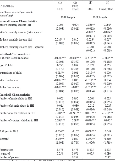
Table A2. OLS and Fixed Effect Estimates of Child Labor Hours (Full Sample)
Father's monthly income (ln) 0.004 -0.004 0.026** 0.060*
(0.003) (0.011) (0.012) (0.036)
Father's monthly income (ln) – squared -0.001* -0.004*
(0.001) (0.002)
Mother's monthly income (ln) 0.010*** 0.010 0.023* 0.067
(0.002) (0.007) (0.012) (0.041)
Mother's monthly income (ln) – squared -0.001 -0.004
(0.001) (0.003)
Individual Characteristics
=1 if child is still in school -0.678*** -0.880*** -0.678*** -0.868*** (0.106) (0.192) (0.106) (0.192)
Age of child -0.273 0.039 -0.272 0.065
(0.170) (0.295) (0.170) (0.296)
Squared age of child 0.015** 0.001 0.015** 0.000
(0.007) (0.012) (0.007) (0.012)
Father’s education -0.012*** 0.005 -0.011*** 0.004
(0.004) (0.019) (0.004) (0.019)
Mother’s education -0.012*** -0.017 -0.011*** -0.012
(0.004) (0.033) (0.004) (0.033)
Household Characteristics
Number of male adults in HH -0.003 0.030 -0.004 0.025
(0.015) (0.054) (0.015) (0.055)
Number of female adults in HH -0.015 -0.030 -0.012 -0.027
(0.016) (0.048) (0.016) (0.049) Number of older children in HH 0.083*** -0.243*** 0.083*** -0.238***
(0.032) (0.066) (0.032) (0.066) Number of younger children in HH 0.091*** -0.097* 0.090*** -0.092* (0.015) (0.055) (0.015) (0.055)
=1 if year is 2014 0.056** -0.107 0.069*** -0.048
(0.025) (0.077) (0.025) (0.081)
Source: Author’s analysis based on IFLS4 (2007) and IFLS5 (2014).
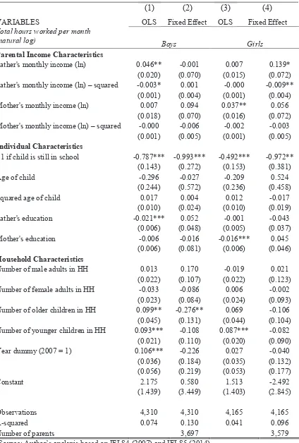
Table A3. OLS and Fixed-Effects Estimates of Child Labor Hours: Boys vs Girls
(1) (2) (3) (4)
VARIABLES OLS Fixed Effect OLS Fixed Effect
Total hours worked per month
(natural log) Boys Girls
Parental Income Characteristics
Father's monthly income (ln) 0.046** -0.001 0.007 0.139* (0.020) (0.070) (0.015) (0.072) Father's monthly income (ln) – squared -0.003* 0.001 -0.000 -0.009**
(0.001) (0.004) (0.001) (0.004) Mother's monthly income (ln) 0.007 0.094 0.037** 0.056
(0.018) (0.070) (0.016) (0.072) Mother's monthly income (ln) – squared -0.000 -0.006 -0.002 -0.003
(0.001) (0.005) (0.001) (0.005)
Individual Characteristics
=1 if child is still in school -0.787*** -0.993*** -0.492*** -0.972** (0.143) (0.272) (0.153) (0.381)
Age of child -0.296 -0.027 -0.209 0.524
(0.244) (0.572) (0.236) (0.458)
Squared age of child 0.017 0.004 0.012 -0.017
(0.010) (0.024) (0.010) (0.019)
Father's education -0.021*** 0.052 -0.001 -0.043
(0.006) (0.048) (0.005) (0.037)
Mother's education -0.006 -0.016 -0.016*** 0.045
(0.006) (0.081) (0.006) (0.046)
Household Characteristics
Number of male adults in HH 0.013 0.170 -0.019 0.021 (0.022) (0.107) (0.022) (0.123) Number of female adults in HH -0.033 -0.086 0.006 -0.002
(0.023) (0.084) (0.024) (0.093) Number of older children in HH 0.099** -0.276** 0.069 -0.106
(0.045) (0.131) (0.044) (0.104) Number of younger children in HH 0.093*** -0.108 0.087*** -0.082
(0.021) (0.110) (0.020) (0.090)
Year dummy (2007 = 1) 0.106*** -0.226 0.027 -0.040
(0.036) (0.184) (0.035) (0.132)
Source: Author’s analysis based on IFLS4 (2007) and IFLS5 (2014)
Table A4. OLS and Fixed Effect Estimates of Child Labor Hours: Rural vs Urban
(1) (2) (3) (4)
VARIABLES OLS Fixed Effect OLS Fixed Effect
Total hours worked per month (natural log)
Urban Rural
Parental Income Characteristics
Father's monthly income (ln) -0.005 0.010 0.051** 0.119** (0.014) (0.052) (0.021) (0.047) Father's monthly income (ln) – squared 0.000 -0.000 -0.003** -0.008***
(0.001) (0.003) (0.001) (0.003) Mother's monthly income (ln) 0.051*** 0.037 -0.001 0.177** (0.015) (0.046) (0.020) (0.073) Mother's monthly income (ln) – squared -0.003*** -0.002 0.001 -0.012**
(0.001) (0.003) (0.001) (0.005)
Individual Characteristics
=1 if child is still in school -0.546*** -0.351 -0.760*** -1.094*** (0.154) (0.260) (0.144) (0.268)
Age of child -0.130 -0.156 -0.423 0.247
(0.206) (0.373) (0.278) (0.482)
Squared age of child 0.008 0.008 0.022* -0.007
(0.009) (0.016) (0.012) (0.020)
Father's education -0.013*** -0.005 -0.002 0.024
(0.005) (0.027) (0.006) (0.035)
Mother's education -0.000 0.027 -0.017** -0.018
(0.005) (0.043) (0.007) (0.052)
Household Characteristics
Number of male adults in HH 0.009 0.118 -0.004 -0.037
(0.018) (0.074) (0.026) (0.087) Number of female adults in HH -0.004 0.021 -0.011 -0.170* (0.019) (0.060) (0.029) (0.101) Number of older children in HH 0.017 -0.287*** 0.141*** -0.218* (0.034) (0.080) (0.052) (0.116) Number of younger children in HH 0.051*** -0.106 0.132*** -0.073
(0.018) (0.071) (0.023) (0.092)
=1 if year is 2014 0.070** -0.151 0.081* 0.122
(0.031) (0.099) (0.042) (0.135)
Source: Author’s analysis based on IFLS4 (2007) and IFLS5 (2014)
Drawing on the substitution axiom formulated by Basu and Van (1998) this study examines the nature of relationship between parental income and child labor supply in Indonesia. To estimate such relationship, we are benefited by panel data from the last two waves of Indonesia Family Life Survey (2007 and 2014). We tackle the potential endogeneity in parental income by controlling for parental fixed-effect. Results shows that parental income matter to child labor supply. The effect of father’s income looks more significant to all sample particularly to girls. In rural areas, both parental income matter to girls, and not to boys. The relationship between a father’s income (and mother’s in rural) with children’s labor hours are complementary at low level of income, and as income rises, the increments in child labor hours decreases and at high levels of income, the relationship transforms into a substitute relationship –resembling an inverted-U shape.
THE NATIONAL TEAM FOR THE ACCELERATION OF POVERTY REDUCTION
Office of the Vice President of the Republic of Indonesia
Jl. Kebon Sirih No. 14, Jakarta Pusat 10110
Phone : (021) 3912812
Fax : (021) 3912511
E-mail : info@tnp2k.go.id