The Democratization of Credit and the Rise in
Consumer Bankruptcies
∗
Igor Livshits
University of Western Ontario, BEROC
James MacGee
University of Western Ontario
Mich`ele Tertilt
University of Mannheim and CEPR
February 28, 2014
Abstract
Financial innovations are a common explanation for the rise in credit card debt and bankruptcies. To evaluate this story, we develop a simple model that incor-porates two key frictions: asymmetric information about borrowers’ risk of default and a fixed cost of developing each contract lenders offer. Innovations that amelio-rate asymmetric information or reduce this fixed cost have large extensive margin effects via the entry of new lending contracts targeted at riskier borrowers. This results in more defaults and borrowing, and increased dispersion of interest rates. Using the Survey of Consumer Finances and Federal Reserve Board interest rate data, we find evidence supporting these predictions. Specifically, the dispersion of credit card interest rates nearly tripled while the “new” cardholders of the late 1980s and 1990s had riskier observable characteristics than existing cardholders. Our cal-culation suggest these new cardholders accounted for over 25% of the rise in bank credit card debt and delinquencies between 1989 and 1998.
Keywords: Credit Cards, Endogenous Financial Contracts, Bankruptcy. JEL Classifications: E21, E49, G18, K35
1
Introduction
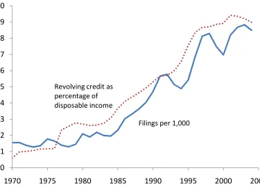
Financial innovations are frequently cited as a key factor in the dramatic increase in households’ access to credit cards between 1980 and 2000. By making intensive use of improved information technology, lenders were able to price risk more accurately and to offer loans more closely tailored to the risk characteristics of different groups (Mann 2006; Baird 2007). The expansion in credit card borrowing, in turn, is thought to be a key force driving the surge in consumer bankruptcy filings and unsecured borrowing (see Figure 1) over the past thirty years (White 2007).
Surprisingly little theoretical work, however, has explored the implications of finan-cial innovations for unsecured consumer loans. We help fill this gap by developing an incomplete markets model of bankruptcy to analyze the qualitative implications of improved credit technology. To guide us in assessing the model’s predictions, we doc-ument that many key innovations in the U.S. credit card industry occurred during the mid-1980s to the mid-1990s. This leads us to compare the model’s predictions to cross-sectional data on the evolution of credit card debt and interest rates during these years. Our model incorporates two frictions that are key in shaping credit contracts: asym-metric information about borrowers’ default risk, and a fixed cost of creating a credit contract. While asymmetric information is a common element of credit models, fixed costs of contract design have been largely ignored by the academic literature.1 This is surprising, as texts targeted at practitioners document significant fixed costs. According to Lawrence and Solomon (2002), a prominent consumer credit handbook, developing a consumer lending product involves selecting the target market, designing the terms and conditions of the product and scorecards to assess applicants, testing the product, fore-casting profitability, and preparing formal documentation. Even after the initial launch, there are ongoing overhead costs, such as regular reviews of the product design and scorecards as well as maintenance of customer databases, that vary little with the num-ber of customers. Finally, it is worth noting that fixed costs are consistent with the obser-vation that consumer credit contracts are differentiated but rarely individual-specific.
ceiving a high endowment realization in the second period. To offer a lending contract, which specifies an interest rate, a borrowing limit and a set of eligible borrowers, an intermediary incurs a fixed cost. When designing loan contracts, lenders face an asym-metric information problem, as they observe a noisy signal of a borrower’s true default risk, while borrowers know their type. There is free entry into the credit market, and the number and terms of lending contracts are determined endogenously. To address well known issues related to existence of competitive equilibrium with adverse selection, the timing of the lending game builds on Hellwig (1987). This leads prospective lenders to internalize how their entry decisions impact other lenders’ entry and exit decisions.
The equilibrium features a finite set of loan contracts, each “targeting” a specific pool of risk types. The finiteness of contracts follows from the assumption that a fixed cost is incurred per contract, so that some “pooling” is necessary to spread the fixed cost across multiple types of borrowers. Working against larger pools is that these require a broader range of risk types, leading to wider gaps between the average default rate and the default risk of the least risky pool members. With free entry of intermediaries, these forces lead to a finite set of contracts for any (strictly positive) fixed cost.
We use this framework to analyze the qualitative implications of three channels through which financial innovations may have impacted credit card lending since the mid-1980s: (i) reductions in the fixed cost of creating contracts; (ii) increased accuracy of lenders’ predictions of borrowers’ default risk; and (iii) a reduced cost of lenders’ funds. As we discuss in Section 2, the first two channels capture the idea that improvements in infor-mation technology reduced the cost of designing loan contracts, and allowed lenders to price borrowers’ risk more accurately. The third channel is motivated by the increased use of securitization (which reduced lenders’ costs of funds) and by lower costs of ser-vicing consumer loans following improvements in information technology.
the model, the new contract margin dominates the local effect of smaller pools, so new contracts increase the number of borrowers.
Aggregate borrowing and defaults are driven by the extensive margin, with more borrowers leading to more borrowing and defaults. Changes in the size and number of contracts induced by financial innovations result in more disperse interest rates, as rates for low risk borrowers decline while high risk borrowers gain access to high rate loans. Smaller pools lower the average gap between a household’s default risk and in-terest rate, leading to improved risk-based pricing. This effect is especially pronounced when the accuracy of the lending technology improves, as fewer high risk borrowers are misclassified as low risk.
While all three channels are driven by a common information-intensive innovation in lending technology, a natural question is whether they differ in predictions. One dimension along which improved risk assessment differs from the other channels is the average default rate of borrowers. On the one hand, whenever the number of contracts increases, households with riskier observable characteristics gain access to risky loans. However, an increase in signal accuracy also reduces the number of misclassified high risk types offered loans targeted at low risk borrowers, which lowers defaults. In our numerical example, these effects roughly offset, so that improved risk assessment leaves the average default rate ofborrowersessentially unchanged. Another dimension along which the three channels differ is in their impact on overhead costs. While a decline in the fixed costs leads to a decline in the overhead costs of borrowing, this is not so for the other channels. An increase in signal accuracy and a fall in the cost of funds leads to anincrease of overhead costs (even as a percentage of total loans), as more types of contracts are offered, each with its own fixed cost.
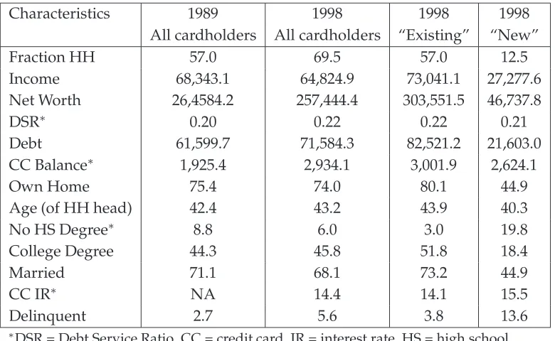
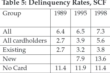
Consistent with the model’s predictions, the jump in the fraction of households with a bank credit card from 43% in 1983, to 56% in 1989 and 68% in 1998, entailed the ex-tension of cards to borrowers with riskier characteristics. Since the SCF is a repeated cross-section, we build on Johnson (2007) and use a probit regression of bank card own-ership on household characteristics in 1989 to identify “new” and ”existing” cardholders in 1998. The “new” cardholders have riskier characteristics, being less likely to be mar-ried, less educated, and have lower income and net worth – and higher interest rates and delinquency rates. Building on this exercise, we conclude that the new cardholders account for roughly 25% of the increase in credit card debt from 1989 to 1998. We con-duct a similar exercise to quantify the contribution of the new cardholders to the rise in delinquencies (a proxy for increased bankruptcy risk). We find that between a quarter and a third of the rise can be attributed to the extensive margin of new cardholders.
Our empirical results on the quantitative importance of the extensive margin of new cardholders for the rise in credit card debt and bankruptcy may surprise some. A widespread view among economists is that the rise in bankruptcy was due primarily to either an intensive margin of low risk borrowers taking on more debt (e.g. Nara-jabad (2012), Sanchez (2012)) or a fall in thestigma of bankruptcy (Gross and Souleles 2002). Interestingly, our empirical exercise yields results forexistingcardholders similar to those of Gross and Souleles (2002) who found that the default probability, controlling for risk measures, of a sample of credit card borrowers jumped between June 1995 and June 1997. Thus, our empirical findings suggest that the rise in bankruptcy over the 1990s can be accounted for largely by the extensive margin and lower “stigma”.
for their empirical findings. By lowering barriers to interstate banking, deregulation ex-pands market size, effectively lowering the fixed cost of contracts. In our framework, this leads to the extension of credit to riskier borrowers, resulting in more bankruptcies.
Our framework also offers new insights into the debate over the welfare implications of financial innovations. In our environment, financial innovations increase average (ex ante) welfare but are not Pareto improving, as changes in the size of contracts result in some households being shifted to higher interest rate contracts. Moreover, the compet-itive allocation in general is not efficient, as it features more contracts and less cross-subsidization than would be chosen by a social planner who weights all households equally. This results in the financial sector consuming more resources than is optimal.
This paper is related to the incomplete market framework of consumer bankruptcy of Chatterjee et al. (2007) and Livshits, MacGee, and Tertilt (2007).2 Livshits, MacGee, and Tertilt (2010) and Athreya (2004) quantitatively evaluate alternative explanations for the rise in bankruptcies and borrowing. Both papers conclude that changes in con-sumer lending technology, rather than increased idiosyncratic risk (e.g., increased earn-ings volatility), are the main factors driving the rise in bankruptcies.3 Unlike this paper, they abstract from how financial innovations change the pricing of borrowers’ default risk, and model financial innovation as a fall in the “stigma” of bankruptcy and a decline in lenders’ cost of funds. Hintermaier and Koeniger (2009) find changes in the risk-free rate have little impact on unsecured borrowing and bankruptcies.
Closely related in spirit is complementary work by Narajabad (2012), Sanchez (2012), Athreya, Tam, and Young (2012), and Drozd and Nosal (2008). Narajabad (2012), Sanchez (2012) and Athreya, Tam, and Young (2012) examine improvements in lenders’ ability to predict default risk. In these papers, more accurate or cheaper signals lead to relatively lower risk households borrowing more (i.e., an intensive margin shift), which increases their probability of defaulting. Drozd and Nosal (2008) examine a fall in the fixed cost incurred by the lender to solicit potential borrowers, which leads to lower interest rates and increased competition for borrowers. Our work differs from these papers in sev-eral key respects. First, we introduce a novel mechanism which operates through the extensive rather than intensive margin. Second, our tractable framework allows us to derive closed form solutions and thereby provides insights into the mechanism, while
the previous literature has focused on complex quantitative models. Third, we docu-ment several novel facts on the evolution of the credit card industry.
Also related to this paper is recent work on competitive markets with adverse selec-tion. Adams, Einav, and Levin (2009), Einav, Jenkins, and Levin (2012) and Einav, Jenk-ins, and Levin (2009) find that subprime auto lenders face moral hazard and adverse selection problems when designing the pricing and contract structure of auto loans, and that there are significant returns to improved technology to evaluate loan applicants (credit scoring). Earlier work by Ausubel (1999) also found that adverse selection is present in the credit card market. Recent work by Dubey and Geanakoplos (2002), Guer-rieri, Shimer, and Wright (2010) and Bisin and Gottardi (2006) considers existence and efficiency of competitive equilibria with adverse selection. Our paper differs both in its focus on financial innovations, and its incorporation of fixed costs of creating contracts. The remainder of the paper is organized as follows. Section 2 documents innovations in the credit card industry since the 1980s, and Section 3 outlines the general model. In Section 4 we characterize the set of equilibrium contracts, while Section 5 examines the implications of financial innovations. Section 6 compares these predictions to data on U.S. credit card borrowing, and Section 7 analyzes the quantitative role of the extensive margin. Section 8 concludes. Additional details on the theory and empirical analysis is provided in a supplementary web appendix.
2
Credit Card Industry: Evolution and Driving Forces
2.1
Credit Cards and Credit Scorecards
Credit card lenders today offer highly differentiated cards that vary in pricing (i.e., the interest rate, annual fees and late fees) and other dimensions (e.g., affinity cards). This entails a data-intensive strategy that designs contracts tailored to specific market seg-ments (e.g., see Punch (1998)). In practice, this typically involves a numerically intensive evaluation of the relationship between borrowers’ characteristics and credit risk (using proprietary data and data purchased from credit bureaus). Credit card companies also often undertake lengthy and costly experiments with alternative contract terms.4
Central to this data intensive approach to risk assessment is the use of specially devel-oped credit scorecards.5 Each scorecard is a statistical model (estimated with historical data) mapping consumer characteristics into repayment and default probability for a specific product. Indeed, some large banks use 70 to 80 different scoring models in their credit card operations, with each scorecard adapted to a specific product or market seg-ment (McCorkell 2002). This involves substantial costs; developing, impleseg-menting and managing a (single) customized scorecard can cost from $40,000 to more than $100,000 (see Mays (2004), p. 34).6 Custom scorecards are built in-house or developed by spe-cialized external consultants (e.g., Moody’s Analytics and Risk Management Services and Capital Card Services Inc.).7 While developing scorecards entails significant fixed costs, the resulting automated system reduces the cost of evaluating individual applicants.8
These scorecards are distinct from (and typically supplement) general-purpose credit scores, such as FICO.9 While many lenders use FICO scores as an input to their credit evaluations, it is typically only one piece of information used to evaluate an individual’s credit risk, and is combined with a custom score based on borrower characteristics (with the score often conditioned on the specific product terms). This reflects the limitation of
4Experiments involve offering contract terms to random samples from a target population and tracking borrowing and repayment behaviour (often over 18 to 24 months). Based on these data, lenders adjust the terms and acceptance criteria (see Ausubel (1999) and Agarwal, Chomsisengphet, and Liu (2010)).
5One indication of the wide use of scorecards are the numerous handbooks providing practitioners de-tailed guides on their development (e.g., Lawrence and Solomon (2002), Mays (2004), and Siddiqi (2006)). 6Customized scorecards are updated every few years to account for changes in the applicant popula-tion and macroeconomic condipopula-tions. As a result, scorecard development requires recurring fixed costs.
7Siddiqi (2006) discusses a company that outsourced scorecard development and purchased ten differ-ent cards at an average cost of $27,000 each.
8Citing the Federal Reserve Board (2007): “Credit-scoring systems generally involve significant fixed costs to develop, but their ‘operating’ cost is extremely low – that is, it costs a lender little more to apply the system to a few million cases than it does to a few hundred.”
general-purpose scores, which are designed to predict default probabilities rather than expected recovery rates or expected profitability of different borrowers for a specific contract. As a result, a customized score can improve the accuracy of credit risk assess-ment for borrowers offered a specific product. The estimation of scorecards often uses both lender specific information (e.g., from experiments or client histories) and informa-tion purchased from credit bureaus, such as generic credit scores, borrowers’ repayment behaviour, and borrowers’ debt portfolio.10
2.2
Evolution of the Credit Card Industry
While the idea of systematically using historical data on loan performance to shape loan underwriting standards dates back to Durand (1941), until recently consumer loan offi-cers still relied primarily upon “the 4Cs” (i.e., Character, Capacity, Capital, Collateral) (Smith 1964). This began to change in the late 1960s, as the emergence of credit cards and advances in computing brought the development of application credit scoring models. Pioneered by Fair Isaac, these models provided lenders with generic estimates of the likelihood of serious delinquency in the upcoming year (Thomas 2009).
By the 1980s, advancements in information technology paved the way for a revo-lution in how consumer loans are assessed, monitored and administered (Barron and Staten 2003; Berger 2003; Evans and Schmalensee 2005). With lower costs of compu-tation and data storage, behavioural credit scoring systems that incorporated payment and purchase information and information from credit bureaus, were developed, trig-gering the widespread adoption of credit scoring (McCorkell 2002; Engen 2000; Asher 1994; Thomas 2009).11 These innovations are asserted to have played a key role in the growth of the credit card industry (Evans and Schmalensee 2005; Johnson 1992).12
The 1980s saw new entrants such as MBNA, First Deposit and Capital One build on these advances to design credit card contracts for targeted segments of the popula-tion. Shortly after its founding in 1981 as the firstmonolinecredit card issuer (i.e., lender 10U.S. credit bureaus report borrowers’ payment history, debt and public judgments (Hunt 2006). More than two million credit reports are sold daily by U.S. credit bureaus (Riestra 2002)
11Fair Isaac and Company started building credit scoring systems in the late 1950s. Their first behaviour scoring system was introduced in 1975, first credit bureau score in 1981 and first general-purpose FICO score in 1989. See http://www.fico.com/en/Company/Pages/history.aspx.
specializing in credit cards), MNBA embarked on a strategy of data-based screening of targets and underwriting standards for different credit card products (Cate and Staten 2003). In 1984, First Deposit Corporation13adopted a business model of developing
an-alytic methods of targeting card offers to mispriced demographic groups (i.e., groups with relatively low default probabilities for that product).14 Structured
experimenta-tion was pioneered by Rich Fairbank and Nigel Morris in 1988. Initially working with a regional bank (Signet), they used experiments which involved sending out offers for various products (i.e., credit cards with different terms) to consumers to design differ-entiated credit products for individual market segments (Clemons and Thatcher 1998). This “test and learn” strategy was so successful that in 1994, Signet spun off their group as a monoline lender, Capital One, which became one of the largest U.S. credit card is-suers. Capital One initiated the dynamic re-pricing customer accounts, a practive that required intensive ongoing analysis of customer data (Clemons and Thatcher 2008).
This strategy of using quantitative methods and borrower data to design credit prod-ucts targeted at different groups of borrowers was adopted by other large banks and new monoline lenders throughout the late 1980s and early 1990s.15 By the end of 1996,
42 large monoline lenders accounted for 77% of the total outstanding credit card bal-ances of commercial banks (Federal Reserve Board 1997). The shifting landscape led to changes in the pricing strategy of credit card lenders, with companies such as AmEx in-troducing cards with different interest rates based on customers’ risk.16 This resulted in
declines (increases) in interest rates for lower (higher) risk borrowers (Barron and Staten 2003).17 The 1990s also saw non-bank lenders such as Sears (Discover), GM, AT&T and
GE enter the credit card market to take advantage of proprietary data on their customers.
While the changes in the credit card market are widely discussed, there is
surpris-13Ultimately, it became Providian Financial Corporation, a leading issuer of credit cards.
14Initially developed by Andrew Kahr, their first credit card product targeted low-risk“revolvers” by
dropping the annual fee, upped the interest rate to 22%, lowering the minimum monthly payment, and offering new customers a cash-advance loan (at a high interest rate). Four years after opening, First Deposit had over 350,000 customers and $1 billion in credit card receivables (Nocera (1994), pp 315-324).
15A proxy for this diffusion is the fraction of large banks using credit scoring in loan approval, which
rose from 50% in 1988 to 85% in 2000 (American Bankers Association 2000). Similarly, the fraction of large banks using fully automated loan processing (for direct loans) increased from 12% in 1988 to nearly 29% in 2000 (American Bankers Association 2000). While larger banks often customize their own scorecards, smaller banks adopted this technology by purchasing scores from specialized providers (Berger 2003).
16In 1992, AmEx’s Optima card charged prime rate plus 8.25% from its new customers, prime plus 6.5%
from its best customers, and prime plus 12.25% from chronic late-payers (Canner and Luckett 1992).
17A similar finding holds for small business loans, where the adoption of credit scoring led to the
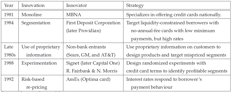
Table 1: Credit Card Evolution Timeline
Year Innovation Innovator Strategy
1981 Monoline MBNA Specializes in offering credit cards nationally.
1984 Segmentation First Deposit Corporation Target liquidity-constrained borrowers with
(later Providian) no-annual-fee cards with low minimum
payments, but high rates
Late Use of proprietary Non-bank entrants Use proprietary information on customers to
1980s information (Sears, GM, and AT&T) design products and target mispriced segments
1988 Experimentation Signet (later Capital One) Design randomized experiments with
R. Fairbank & N. Morris credit card terms to identify profitable segments
1992 Risk-based AmEx (Optima card) Interest rates respond to borrower’s
re-pricing payment behaviour
Sources: See text, Section 2.2.
ingly little quantitative documentation of the diffusion of new practices.18 To document the timing of the diffusion of new lending technologies, we collected data on references to credit scoring in various publications. Figure 2(a) plots normalized counts of the words “credit scoring” and “credit score” in trade journals, the business press and aca-demic publications.19 The figure shows a dramatic rise in references to credit scoring in the professional press after 1987. UsingGoogleScholarto count mentions in Business, Finance, and Economics publications, we find a similar trend (see Figure 2(b)). Together, these measures paint a clear picture: credit scoring was negligible in the 1970s, picked up in the 1980s and accelerated in the mid 1990s.
2.3
Underlying Factors
Thus far, we have documented key innovations in the credit card industry — the de-velopment of customized scorecards and greater use of detailed borrower data to price borrower risk. Why did these innovations take hold in the 1980s and ’90s? Modern credit scoring is a data-intensive exercise that requires large data sets (of payment his-18This is a common challenge: “A striking feature of this literature [...] is therelative dearth of empirical
studiesthat [...] provide a quantitative analysis of financial innovation.” Frame and White (2004).
19More specifically, the figure displays the word count relative to the counts of the phrase “consumer
tories and borrower characteristics) and rapid computing to analyze them (Giannasca and Giordani 2013). Thus, technological improvements in IT that shrunk the costs of data storage and processing were an essential prerequisite for the development and widespread adoption of credit scoring (McCorkell 2002; Engen 2000; Asher 1994).
The dramatic decline in IT costs in the second half of the 20th century is illustrated by the IT price index constructed by Jorgenson (2001) (Figure 2(c)), and by data on the cost of computing from Nordhaus (2007) (Figure 2(d)). Coughlin, Waid, and Porter (2004) report that the cost per MB of storage fell by a factor of roughly 100 between 1965 and the early 1980s, before falling even faster over the next twenty years. Lower IT and data storage costs led to the digitization of consumer records in the 1970s, in turn reducing the cost of developing and using credit scoring tools to assess risk (Poon 2011).
Another key development in the credit industry related to how credit card compa-nies finance their operations. Beginning in 1987, lenders began to securitize credit card receivables. Securitization increased rapidly, with over a quarter of bank credit card bal-ances securitized by 1991, and nearly half by 2005 (Federal Reserve Board 2006). This facilitated the rapid growth of monolines, and helped lower financing costs for some credit card lenders (Furletti 2002; Getter 2008).
3
Model Environment
We analyze a two-period small open economy populated by a continuum of borrowers, who face a stochastic endowment in period 2. Markets are incomplete as only non-contingent contracts can be issued. However, borrowers can default on contracts by paying a bankruptcy cost. Financial intermediaries can access funds at an (exogenous) risk-free interest rater.
3.1
People
Borrowers live for two periods and are risk-neutral, with preferences represented by:20
c1+βEc2.
Each household receives the same deterministic endowment ofy1units of the
consump-tion good in period 1. The second period endowment,y2, is stochastic taking one of two
possible values: y2 ∈ {yh, yl}, where yh > yl.21 Households differ in their probabilityρ
of receiving the high endowmentyh. We identify households with their typeρ, which is distributed uniformly on[0,1].22 While borrowers know their own type, lenders do not observe it. However, upon paying a fixed cost (discussed below), the lenders get a signal σregarding a borrower’s type. With probability α, this signal is accurate: σ = ρ. With probability(1−α), the signal is an independent draw from theρdistribution (U[0,1]).
We assume β < q¯ = 1
1+r, so that households want to borrow at the risk-free rate. Households’ borrowing, however, is limited by their inability to commit to repayment.
3.2
Bankruptcy
There is limited commitment by borrowers who can choose to declare bankruptcy in period 2. The cost of bankruptcy to a borrower is the loss of fractionγ of the second-period endowment. Lenders do not recover any funds from defaulting borrowers.
20Linearity of the utility function allows a clean characterization of the unique equilibrium. Using CRRA preferences would complicate the analysis, as different types within a contract interval could dis-agree about the optimal size of the loan (given the price). While introducing risk aversion would lose the analytical tractability, we believe the main mechanism is robust as fixed costs create an incentive to pool different types into contracts even with strictly concave utility functions.
21While the assumption of two possible income realizations affords us a great deal of tractability (in part by making it easy to rank individual risk types), the key mechanism we highlight carries over to richer environments. That is, as the costs of advancing loans fall, contracts become more “specialized,” and lenders offer risky loans to new (and riskier) borrowers.
3.3
Financial Market
Financial markets are competitive. Financial intermediaries can borrow at the exoge-nously given interest rate r and make loans to borrowers. Loans take the form of one period non-contingent bond contracts. However, the bankruptcy option introduces a partial contingency by allowing bankrupts to discharge their debts.
Financial intermediaries incur a fixed cost χ to offer each non-contingent lending contract to (an unlimited number of) households. Endowment-contingent contracts are ruled out (e.g., due to non-verifiability of the endowment realization). A contract is characterized by(L, q, σ), whereLis the face value of the loan,qis the per-unit price of the loan (so thatqLis the amount advanced in period 1 in exchange for a promise to pay
Lin period 2), andσis a cut-off for which household types qualify for the contract.
The fixed cost of offering a contract is the costs of developing a scorecard (discussed in Section 2.1), which allows the lender to assess borrowers’ risk types. Thus, upon paying the fixed costχ, a lender gets to observe a signalσ of a borrower’s type, which is accurate (equal toρ) with probabilityα. While each scorecard is specific to a contract (that is, it informs a lender whether a borrower’s σ meets a specific threshold σ), the signalσ is perfectly correlated across lenders (and is known to the borrower).23
In equilibrium, the bond price incorporates the fixed cost of offering the contract (so that the equilibrium operating profit of each contract equals the fixed cost) and the default probability of borrowers. Since no risk evaluation is needed for the risk-free contract(γyl, q,0), no fixed cost is required.24 Households can accept only one loan, so
intermediaries know the total amount borrowed.
3.4
Timing
The timing of events is critical for supporting pooling across unobservable types in equi-librium (see Hellwig (1987)). The key idea is that “cream-skimming” deviations are made unprofitable if pooling contracts can exit the market in response.
23Consider, for example, a low-risk borrower who lives in a zip code with mostly high-risk consumers.
If the zip code is an input used for scorecards, all lenders will misclassify this borrower into a high risk category (and the borrower is aware of that). This mechanism also applies to high-risk borrowers with low-risk characteristics (e.g., long tenure with their current employer or at their current address).
24In an earlier version of the paper, we treated the risk-free contract symmetrically. This does not change
1.a. Intermediaries pay fixed costsχof entry and announce their contracts — the stage ends when no intermediary wants to enter given the contracts already announced.
1.b Households observe all contracts and choose which one(s) to apply for (realizing that some intermediaries may choose to exit the market).
1.c Intermediaries decide (using the scorecard) whether to advance loans to applicants or exit the market.
1.d Lenders who chose to stay in the market notify qualified applicants.
1.e Borrowers who received loan offers pick their preferred loan contract. Loans are advanced.
2.a Households realize their endowments and make default decisions.
2.b Non-defaulting households repay their loans.
3.5
Equilibrium
We study (pure strategy) Perfect Bayesian Equilibria of the extensive form game de-scribed in Subsection 3.4. In the complete information case, the object of interest become Subgame Perfect Equilibria, and we are able to characterize the complete set of rium outcomes. In the asymmetric information case, we characterize “pooling” equilib-ria where all risky contracts have the same face value (i.e. equilibequilib-ria that are similar to the full information equilibria) and then numerically verify existence and uniqueness. Details are given in Section 4.2.
An equilibrium (outcome) is a set of active contracts K∗ = {(q
k, Lk, σk)k=1,...,N} and consumers’ decision rulesκ(ρ, σ,K)∈ Kfor each type(ρ, σ)such that
1. Given{(qk, Lk, σk)k6=j}and consumers’ decision rules, each (potential) bankj max-imizes profits by making the following choice: to enter or not, and if it enters, it chooses contract(qj, Lj, σj)and incurs fixed costχ.
2. Given anyK, a consumer of typeρwith public signalσchooses which contract to accept so as to maximize expected utility. Note that a consumer with public signal σcan choose a contractkonly ifσ>σk.
4
Equilibrium Characterization
We begin by examining the environment with complete information regarding house-holds’ risk types (α = 1). With full information, characterizing the equilibrium is rela-tively simple since the public signal always corresponds to the true type. This case is interesting for several reasons. First, this environment corresponds to a static version of recent papers (i.e. Livshits, MacGee, and Tertilt (2007) and Chatterjee et al. (2007)) which abstract from adverse selection. The key difference is that the fixed cost gener-ates a form of “pooling”, so households face actuarially unfair prices. Second, we can analyze technological progress in the form of lower fixed costs. Finally, abstracting from adverse selection helps illustrate the workings of the model. In Section 4.2 we show that including asymmetric information leads to remarkably similar equilibrium outcomes.
4.1
Perfectly Informative Signals
In the full information environment, the key friction is that each lending contract re-quires a fixed costχ to create. Since each borrower type is infinitesimal relative to this fixed cost, lending contracts have to pool different types to recover the cost of creating the contract. This leads to a finite set of contracts being offered in equilibrium.
households are always willing to repay. The risky contracts’ face value is the maximum such that borrowers repay in the high income state. Contracts with lower face value are not offered in equilibrium since, if (risk-neutral) households are willing to borrow at a given price, they want to borrow as much as possible at that price. Formally:
Lemma 4.1. There are at most two loan sizes offered in equilibrium: A risk-free contract with
L=γyland risky contracts withL=γyh.
Risky contracts differ in their bond prices and eligibility criteria. Since the eligibility decision is made after the fixed cost has been incurred, lenders are willing to accept any household who yields non-negative operating profits. Hence, a lender offering a risky loan at price q rejects all applicants with risk type below some cut-off ρ such that the expected return from the marginal borrower is zero: qρL− qL = 0, where ρqL is the expected present value of repayment andqL is the amount advanced to the borrower. This cut-off rule is summarized in the next Lemma:
Lemma 4.2. Every lender offering a risky contract at priceqrejects an applicant iff the expected
profit from that applicant is negative. The marginal type accepted into the contract isρ= qq.
This implies that the riskiest household accepted by a risky contract makes no con-tribution to the overhead cost χ. We order the risky contracts by the riskiness of the clientele served by the contract, from the least to the most risky.
Lemma 4.3. Finitely many risky contracts are offered in equilibrium. Contractnserves
borrow-ers in the interval[σn, σn−1), whereσ0 = 1,σn= 1−n q 2
χ
γyhq, at bond priceqn=qσn.
Proof. If a contract yields strictly positive profit (net ofχ), then a new entrant will enter, offering a better price that attracts the borrowers from the existing contract. Hence, each contractnearns zero profits in equilibrium, so that:
χ=
Lemma 4.3 establishes that each contract serves an interval of borrower types of equal length,25and that the measure pooled in each contract increases in the fixed costχand
the risk-free interest rate, and decreases in the bankruptcy punishmentγyh. If the fixed
cost is so large thatq 2χ
γyh¯q >1, then no risky loans are offered.
The number of risky contracts offered in equilibrium is pinned down by the holds’ participation constraints. Given a choice between several risky contracts, house-holds always prefer the contract with the highestq. Thus, a household’s decision prob-lem reduces to choosing between the best risky contract they are eligible for and the risk-free contract. The value to typeρof contract(q, L)is
vρ(q, L) =qL+β[ρ(yh−L) + (1−ρ)(1−γ)yl],
and the value of the risk-free contract is
vρ(¯q, γyl) = ¯qγyl+β[ρyh+ (1−ρ)yl−γyl].
Note that the right-hand side of equation (4.1) is increasing inρ. Hence, if the participa-tion constraint is satisfied for the highest type in the interval,σn
−1, it will be satisfied for
any household withρ < σn
−1. Solving for the equilibrium number of contracts, N, thus
involves finding the first risky contractnfor which this constraint binds forσn−1.
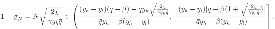
Lemma 4.4. The equilibrium number of contracts offered,N, is the largest integer smaller than:
(yh−yl)[¯q−β(1 +qγy2χhq¯)]
[¯qyh−β(yh−yl)]qγy2χh¯q .
If the expression is negative, no risky contracts are offered.
Proof. We need to find the riskiest contract for which the household at the top of the interval participates: i.e. the largestn such that risk type σn
−1 prefers contract n to the
risk-free contract. Substituting for contractnin the participation constraint (4.1) ofσn
Usingqn =σnq¯andσn= 1−n q
2χ
γyhq from Lemma 4.3, and solving forn, this implies
n ≤
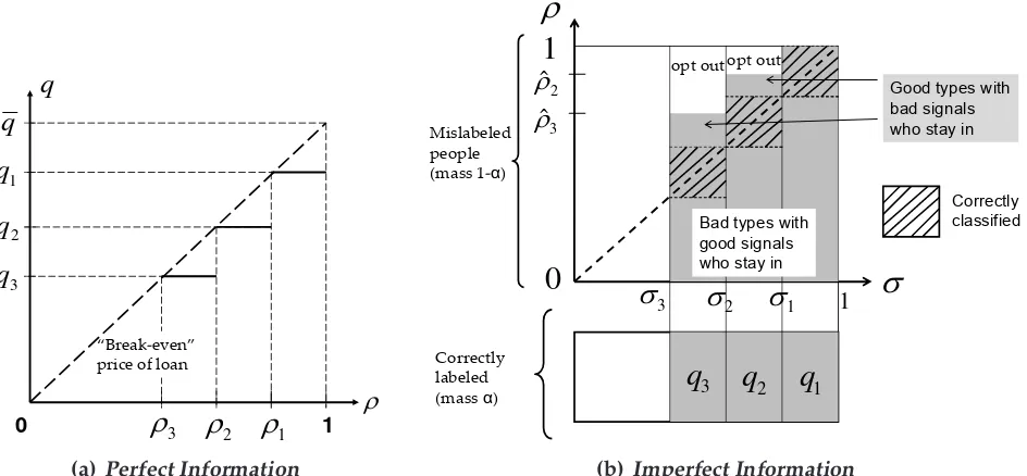
The set of equilibrium contracts is fully characterized by the following theorem, which follows directly from Lemmata 4.1-4.4, and is illustrated in Figure 3(a).
Theorem 4.5. If(¯q−β)[yh−yl] > qy¯ h
. One risk-free contract is offered at priceq¯to all households withρ < σN.
4.2
Incomplete Information
We now characterize equilibria with asymmetric information. We focus on “pooling” equilibria which closely resemble the compete information equilibria of Section 4.1.26
These “pooling” equilibria feature one risk-free contract with loan size L = γyl and
finitely many risky contracts withL=γyh, each targeted at a subset of households with
sufficiently high public signalσ. While we are unable to provide a complete characteri-zation of equilibria with asymmetric information for arbitrary parameter values, we are able to numerically verify that the “pooling” equilibrium is in fact the unique equilib-rium for the parameter values we consider.
The main complication introduced by asymmetric information arises from mislabeled borrowers. The behaviour of borrowers with incorrectly high public signals (σ > ρ) is easy to characterize, since they always accept the contract offered to their public type. Customers with incorrectly low public signals, however, may prefer the risk-free con-tract over the risky concon-tract for their public type. While this is not an issue in the best loan pool (as no customer is misclassified downwards), the composition of riskier pools
26In contrast, a “separating” equilibrium would include smaller risky “separating” loans targeted at
(and thus the pricing) may be affected by the “opt-out” of misclassified low risk types. For each risky contract, denoteρˆn the highest true type willing to accept that contract
over a risk-free loan. Using the participation constraints, we have:
ˆ
ρn =
qnyh−qyl
β(yh−yl)
. (4.2)
Sinceρˆnis increasing inqn, lower bond prices result in a higher opt-out rate. Households
who decline risky loans (i.e., those with public signalσ∈[σn, σn−1)and true typeρ >ρˆn)
borrow via the risk free contract. Figure 3(b) illustrates the set of equilibrium contracts.
Despite this added complication, the structure of equilibrium loan contracts remain remarkably similar to the full information case. Strikingly, as the following lemma es-tablishes, the intervals of public signals served by the risky contracts are of equal size.
Lemma 4.6. In a “pooling” equilibrium, the interval of public types served by each risky contract
is of sizeqαqγy2χh.
Proof. This result follows from the free entry and uniform type distribution assump-tions. Consider an arbitrary risky contract. For any public type σ, let Eπ(σ) denote expected profits. Note that the lowest public type acceptedσ, yields zero expected prof-its. Free entry implies the contract satisfies the zero profit condition, so total profits from the interval of public types betweenσandσ+θ must equalχ.
Z θ
0
Eπ(σ+δ)dδ=χ (4.3)
With probabilityαthe signal is correct (soρ=σ), while with probability1−αthe signal is incorrect, in which case typesρ > ρˆchoose to opt out. To determine the profit from typeσ+δ, note that the fraction of households that do not opt out isα+ (1−α)ˆρ. Hence:
Eπ(σ+δ) = (α+ (1−α)ˆρ)Eπ(σ+δ|ρ <ρˆ)
= (α+ (1−α)ˆρ) [qE(ρ|σ =σ+δ, ρ <ρˆ)γyh−qnγyh].
The additional repayment probability from public type σ + δ over type σ is α+(1−αδα)ˆρ, which is simply the probability that the signal is correct times the difference in repay-ment rates corrected for the measure that accepts the contract (α+ (1−α)ˆρ). Thus:
Eπ(σ+δ) = (α+ (1−α)ˆρ)
αδq
α+ (1−α)ˆργyh+q(E(ρ|σ=σ, ρ <ρˆ))γyh−qnγyh
At the bottom cutoff,σ < σ+θ ≤ ρˆ. Thus, the last two terms equal the expected profit
ging this into equation (4.3), we haveRθ
0 αqγyhδdδ =χ. It follows thatθ =
q 2
χ αqγyh.
The expression for the length of the interval (of public types) served closely resembles the complete information case in Lemma 4.3. The only difference is that less precise signals increase the interval length by the multiplicative factorp1/α. This is intuitive, as the average profitability of a type decreases as the signal worsens, and thus larger pools are needed to cover the fixed cost. What is surprising is that the measure of public types targeted by each contract is the same, especially since the fraction who accept varies due to misclassified borrowers opting out. As the proof of Lemma 4.6 illustrates, this is driven by two effects that exactly offset each other: lower-ranked contracts have fewer borrowers accepting, but make up for it through higher profit per borrower. As a result, the profitability of a type(σ+δ)is the same across contracts (=αδqγyh).
As in the full information case, the number of risky contracts offered in equilibrium is pinned down by the household participation constraints. Typeρis willing to accept risky contract(q, L)whenevervρ(q, L)≥vρ(¯q, γyl). This also implies that if then-th risky
contract(qn, γyh, σn)is offered, thenρˆn > σn−1. That is, no accurately labeled customer ever opts out of a risky contract in equilibrium. Combining Lemma 4.6 with the zero marginal profit condition, one can derive a relationship between the bond price and the cutoff public type for each contract. The next theorem summarizes this result.
Theorem 4.7. Finitely many risky contracts are offered in a “pooling” equilibrium. The n
-th contract(qn, γyh, σn)serves borrowers with public signals in the interval [σn, σn−1), where
whereρˆn is given by equation (4.2). If the participation constraints of mislabeled borrowers do
not bind (ˆρn= 1), this simplifies to qn =q ασn+ (1−α)
1 2
.
possibility of profitable entry of new (separating) contracts. Specifically, one needs to rule out “cream skimming” deviations targeted at borrowers whose public signals are lower than their true type. Such deviation contracts necessarily involve smaller loans offered at better terms, since public types that are misclassified downwards must prefer them to the risk-free contract and true types must prefer the risky contract they are eligible for. In the numerical examples, we computationally verify that such deviations are not profitable. The fixed cost plays an essential role, as it forces potential entrant to “skim” enough people to cover the fixed cost. See Appendix A for a detailed description of the possible deviation and verification procedure.
By numerically ruling out these deviations we also establish that “pooling” is the unique equilibrium. Given our timing assumptions, the existence of a “separating” equi-librium would rule out the “pooling” equiequi-librium, since “separating” is preferred by the best customers (highestρ’s). Uniqueness within the class of “pooling” equilibria follows from the same argument given for the complete information case in Section 4.1.
5
Implications of Financial Innovations
In this section, we analyze the model implications for three channels through which fi-nancial innovations could impact consumer credit: (i) a decline in the fixed costχ, (ii) a decrease in the cost of loanable funds q, and (iii) an improvement in the accuracy of¯
the public signal α. Given the stylized nature of our model, we focus on the qualita-tive predictions for borrowing, defaults, interest rates and the composition of borrow-ers. We find that all three channels affect the extensive margin of who has access to credit. “Large enough” innovations lead to more credit contracts, access to risky loans for higher risk households, more disperse interest rates, more borrowing, and defaults. Each of these channels have different implications for changes in the ratio of overhead cost to total loans and the average default rate of borrowers.
5.1
Decline in the Fixed Cost
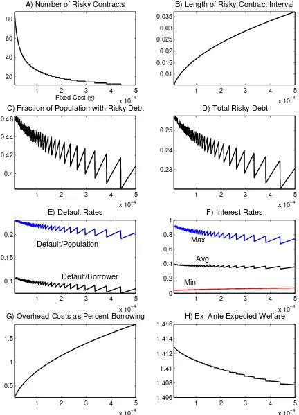
analytical results from Section 4.1, and an illustrative numerical example (see Figure 4), to explore how the model predictions vary withχ.27 For simplicity, we focus on the full
information case (α = 1). Qualitatively similar results hold whenα <1.
A decline in the fixed cost of creating a contract, χ, impacts the set of equilibrium contracts via both the measure served by each contract and the number of contracts (see Figure 4.A and B). Since each contract is of length qγy2χhq, holding the number of con-tracts fixed, a reduction inχreduces the total measure of borrowers. However, a large enough decline in the fixed cost lowers the borrowing rates for (previously) marginal borrowers enough that they prefer the risky to the risk-free contract. This increase in the number of contracts introduces discontinuous jumps in the measure of risky borrow-ers. Globally (for sufficiently large changes inχ), the extensive margin of an increase in the number of contracts dominates, so the measure of risky borrowers increases. This follows from Theorem 4.5, as the measure of risky borrowers is bounded by:
1−σ
Note that the global effect follows from the fact that both the left and the right bound-aries of the interval are decreasing inχ.
Since all risky loans have the same face valueL=γyh, variations inχaffect credit
ag-gregates primarily through the extensive margin of how many households are eligible. As a result, borrowing and defaults inherit the “saw-tooth” pattern of risky borrowers (see Figure 4.C, D and E). However, the fact that new contracts extend credit to riskier borrowers leads (globally) to defaults increasing faster than borrowing. The reason is that the amount borrowed, qnL, for a new contract is lower than for existing contracts
since the bond price is lower. Hence, the amount borrowed rises less quickly than does the measure of borrowers (compare Figure 4.C with 4.D). Conversely, the extension of credit to riskier borrowers causes total defaults (Rσ1
N(1
faster, leading to higher default rates (see Figure 4.E).
The rise in defaults induced by lowerχis accompanied by a tighter relationship be-tween individual risk and borrowing interest rates. The shrinking of each contract inter-val lowers the gap between the average default rate in each pool and each borrower’s default risk, leading to more accurate risk-based pricing. As the number of contracts
increases, interest rates become more disperse and the average borrowing interest rate slightly increases. This reflects the extension of credit to riskier borrowers at high inter-est rates, while interinter-est rates on existing contracts fall (see Figure 4.F).
There are two key points to take from Figure 4.G, which plots total overhead costs as a percentage of borrowing. First, overhead costs in the example are very small. Second, even though χfalls by a factor of 50, total overhead costs (as % of debt) fall only by a
factor of 7. The smaller decline in overheads costs is due to the decrease in the measure served by each contract, so that each borrower has to pay a larger share of the overhead costs. This suggests that cost of operations of banks (or credit card issuers) may not be a good measure of technological progress in the banking sector.
The example also highlights a novel mechanism via which interstate bank deregula-tion could impact consumer credit markets. In our model, an increase in market size is analogous to a lowerχ, since what matters is the ratio of the fixed cost to the measure
of borrowers. Thus, the removal of geographic barriers to banking across geographic regions, which effectively increases the market size, acts similarly to a reduction in χ
and results in the extension of credit to riskier borrowers. This insight is particularly interesting given recent work by Dick and Lehnert (2010), who find that interstate bank deregulation (which they suggest increased competition) was a contributing factor to the rise in consumer bankruptcies. Our example suggests that deregulation may have led to more bankruptcies not by increasing competition per se, but by facilitating in-creased market segmentation by lenders. This (for large enough changes) leads to the extension of credit to riskier borrowers, and thus more bankruptcies.28
5.2
Decline in the Risk Free Rate
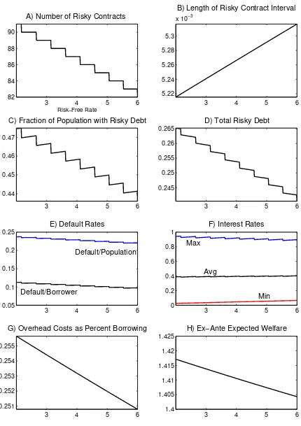
Another channel through which financial innovations may have affected consumer credit is by lowering lenders’ cost of funds, either via securitization or lower costs of loan pro-cessing. To explore this channel, we vary the risk free interest rate in our model. For simplicity, we again assume thatα= 1, although similar results hold forα <1.
The effect of a decline in the risk free rate is similar to a decline in fixed costs. Once again, the measure of borrowers depends upon how many contracts are offered and the
28Bank deregulation and improved information technology may explain the increased role of large
measure served by each contract. The length of each contract isq 2χ
αyhγq, so a lower
risk-free interest rate leads to fewer borrowers per contract. Intuitively, the pass-through
of lower lending costs to the bond priceqn makes the fixed cost smaller relative to the
amount borrowed. Since the contract size depends on the trade-off between spreading the fixed cost across more households versus more cross-subsidization across borrow-ers, the effective reduction in the fixed cost induces smaller pools. Sufficiently large declines in the risk-free rate increase the bond price (qn+1) of the marginal risky contract
by enough that borrowers prefer it to the risk-free contract. Since the global effect of ad-ditional contracts dominates the local effect of smaller pools, sufficiently large declines in the cost of funds lead to more households with risky loans (see Figure 5.A and B).
As with χ, credit aggregates are affected primarily through the extensive margin.
Since increasing the number of borrowers involves the extension of risky loans to riskier borrowers, globally default rates rise with borrowing (see Figure 5.D and E). The av-erage borrowing interest rate reflects the interaction between the pass-through of lower cost of funds, the change in the composition of borrowers, and increased overhead costs. For each existing contract, the lending rate declines by less than the risk-free rate since with smaller pools the fixed cost is spread across fewer borrowers. Working in the op-posite direction is the entry of new contracts with high interest rates, which increases the maximum interest rate (see Figure 5.F). As a result, the average interest rate on risky loans declines by less than 1 point in response to a 4 point decline in the risk-free rate.
This example offers interesting insights into the debate over competition in the U.S. credit card market. In an influential paper, Ausubel (1991) documented that the decline in risk-free interest rates in the 1980s did not result in lower average credit card rates. This led some to claim that the credit card industry was imperfectly competitive. In contrast, Evans and Schmalensee (2005) argued that measurement issues associated with fixed costs of lending and the expansion of credit to riskier households during the late 1980s implied that Ausubel’s observation could be consistent with a competitive lending market. Our model formalizes this idea.29 As Figure 5.F illustrates, a decline in the risk-free interest rate can leave the average interest rate largely unchanged, as cheaper credit pulls in riskier borrowers, which increases the risk-adjusted interest rate.
29Brito and Hartley (1995) formalize a closely related mechanism, but with an exogenously fixed
5.3
Improvements in Signal Accuracy
The last channel we consider is an improvement in lenders’ ability to assess borrowers’ default risk. This is motivated by the improvement of credit evaluation technologies (see Section 2), which maps naturally into an increase in signal accuracy,α. We again use our numerical example to help illustrate the model predictions (see Figure 6).30
Variations in signal accuracy (α) impact who is offered and who acceptsrisky loans. As in Sections 5.1 and 5.2, the measure offered a risky loan depends upon the number and “size” of each contract. From Theorem 4.7, the measure eligible for each contract (qαqγy2χh) is decreasing inα (see Figure 6.B). Intuitively, higherαmakes the credit tech-nology more productive, which results in it being used more intensively to sort borrow-ers into smaller pools. Higherαalso pushes up bond prices (qn) by lowering the number
of misclassified high risk types eligible for each contract. This results in fewer misclassi-fied low risk households declining risky loans, narrowing the gap between the measure accepting versus offered risky loans (see Figure 6.C). A sufficiently large increase inα
raises the bond price of the marginal risky contract enough that it is preferred to the risk-free contract, resulting in a new contract being offered (see Figure 6.A). Globally, the extensive margin of the number of contracts dominates, so the fraction of the popu-lation offered a risky contract increases with signal accuracy.
More borrowers leads to an increase in debt. Similar to a decline in the fixed cost of contracts, an increase in the number of contracts involves the extension of credit to higher risk (public) types, which increases defaults (Figure 6.E). However, the impact of higherαon the default rate of borrowers is more nuanced, as the extension of credit to riskier public types is partially offset by fewer misclassified high risk types. These offsetting effects can be seen in the expression for total defaults (Equation 5.1).
Defaults=α
Asα increases, the rise in the number of contracts (N) lowers σN, which leads to more defaults by correctly classified borrowers. However, higherαalso lowers the number of misclassified borrowers, who are riskier on average than the correctly classified. In our example, this results in the average default rate of borrowers varying little in response to
α, so that total defaults increase proportionally to the total number of (risky) borrowers.
Figure 6.F shows that interest rates fan out asαrises, with the minimum rate declin-ing, while the highest rises. This again reflects the offsetting effects of improved risk assessment. By reducing the number of misclassified borrowers, default rates for ex-isting contracts decline, which lowers the risk premium and thus the interest rate. The maximum interest rate, in contrast, rises (globally) since increases inαlead to new con-tracts targeted at riskier borrowers. Finally, since the average default rate for borrowers is relatively invariant toα, so is the average risk premium (and thus the average inter-est rate). Overall, higherαleads to a tighter relationship between (ex-post) individual default risk and (ex-ante) borrowing interest rates.
Total overhead costs (as a percentage of risky borrowing) increase withα(Figure 6.G), which reflects more intensive use of the lending technology induced by its increased ac-curacy. As a consequence, equating technological progress with reduced cost of lending can be misleading, since technological progress (in the form of an increase inα) may
increase overhead costs.
5.4
Financial Innovations and Welfare
The welfare effects of the rise in consumer borrowing and bankruptcies, and financial innovations in general, have been the subject of much discussion (Tufano 2003; Athreya 2001). In our model, we find that financial innovations improve ex-ante welfare, as the gains from increased access to credit outweigh higher deadweight default costs and overhead lending costs. However, financial innovations are not Pareto improving, as some borrowers are disadvantaged ex-post.
default premium which reduces other borrowers’ interest rates. Overall, this means that the direct effect of innovation on borrowing rates dominate.
While financial innovations increaseex-antewelfare, they are not Pareto improving as they generate both winners and losers ex-post (i.e., once people know their type(ρ, σ)). When the length of the contract intervals shrink, the worst borrowers in each contract (those near the bottom cut-offσn) are pushed into a higher interest rate contract. Thus,
these borrowers always lose (locally) from financial innovation. While this effect holds with and without asymmetric information, improved signal accuracy adds an additional channel via which innovation creates losers. Asαincreases, some borrowers who were
previously misclassified with high public signal become correctly classified, and as a result face higher interest rates (or, no access to risky loans). Conversely, borrowers who were previously misclassified “down” benefit from better borrowing terms as do (on average) correctly classified risk types.
Although financial innovations are welfare improving, the competitive equilibrium allocation is not constrained efficient.31 Formally, we consider the problem of a social
planner who maximizes the ex-ante utility of borrowers before types (ρ, σ) are realized,
subject to the technological constraint that each (risky) lending contract offered incurs fixed costχ.32 The constrained efficient allocation features fewer contracts, each serving
more borrowers, than the competitive equilibrium. Rather than using the zero expected profit condition to pin down the eligibility set (Proposition 4.2), the planner extends the eligibility set of each contract to include borrowers who deliver negative expected prof-its while making the best type (within the contract eligibility set) indifferent between the risky contract and the risk-free contract (i.e. equation (4.1) binds). Since this allocation “wastes” fewer resources on fixed costs, average consumption is higher.
This inefficiency is not directly related to adverse selection, as the perfect information equilibrium is also inefficient.33 Instead, this inefficiency is analogous to the business
stealing effectof entry models with fixed costs where the competitive equilibrium suffers from excess entry (Mankiw and Whinston 1986). Borrowers would like to commit to
31This contrasts with the constrained efficiency result in Allen and Gale (1989). The key difference
be-tween their model and ours arises from the option to pool multiple borrowers to cover the fixed cost of issuing a loan (security). In our model, the inefficiency arises from the creation of too many (i.e. ineffi-ciently small) pools, which does not occur in Allen and Gale (1989) as pooling is ruled out.
32See the web appendix for the explicit representation and solution characterization.
33Since borrowers are risk-neutral there are no direct welfare gains from increased ex post
larger pools with greater cross-subsidization ex-ante (before their type is realized); but ex post some borrowers prefer the competitive contracts. This highlights the practical challenge of improving upon the competitive allocation, as any such policy would make some borrowers worse off and essentially requires a regulated monopolist lender.
6
Comparing the Model Predictions to the Data
In this section, we ask whether the empirical evidence is consistent with three key model predictions of the effect of financial innovation: (i) an increase in the “variety” (number) of credit contracts, (ii) increased access to borrowing for riskier borrowers, and (iii) an increase in risk-based pricing.34 Motivated by the evidence in Section 2, we focus on developments in the credit card market between the mid-1980s and 2000. Subsection 6.1 documents a surge in the number of credit card products during this period. In subsection 6.2 we show that the rise in the fraction of households with access to credit involved the extension of cards to riskier borrowers. Finally, subsection 6.3 outlines evidence of an increase in risk-based pricing since the late 1980s. Our conclusion is that these key model predictions are broadly consistent with the timing of the changes in the credit card industry documented in Section 2.
6.1
Increased Variety in Consumer Credit Contracts
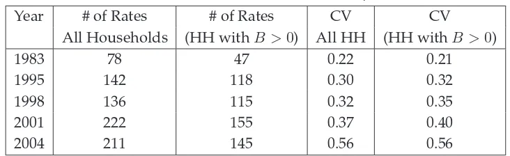
The three financial innovations we consider all predict an increase in the number of risky contracts. In our model, a rise in product variety manifests as an increase in the number of different interest rates offered and as a larger spread between the average and maximum rates. We find a similar trend in the data: the number of different credit card interest rates offered to consumers has increased, the distribution (across borrowers) has become more dispersed and the gap between the average and maximum rate has risen. We use data from the Survey of Consumer Finances (SCF) on the interest rate paid on credit cards to count the number of different interest rates reported. The second and third columns of Table 2 show that the number of different interest rates reported nearly
34The underlying model-implied changes result from an increase inα, a decrease inχor lower cost of
tripled between 1983 and 2004.35 This has been accompanied by increased dispersion
across households as the coefficient of variation (CV) also nearly tripled.36
Table 2: Credit Card Interest Rates, SCF
Year # of Rates # of Rates CV CV
All Households (HH withB >0) All HH (HH withB >0)
1983 78 47 0.22 0.21
1995 142 118 0.30 0.32
1998 136 115 0.32 0.35
2001 222 155 0.37 0.40
2004 211 145 0.56 0.56
Source: Authors’ calculations based on Survey of Consumer Finances.
Comparing the empirical density of interest rates demonstrates this point even more clearly. Figure 7 displays the fraction of households reporting different interest rates in the SCF for 1983 and 2001. It is striking that in 1983 more than 50% of households faced a rate ofexactly18%. The 2001 distribution (and other recent years) is notably “flatter” than that of 1983, with no rate reported by more than 12% of households.
We also find increased dispersion in borrowing interest rates from survey data col-lected from banks by the Board of Governors on credit card interest rates and 24-month consumer loans.37 As can be seen from Figure 8(a), the CV for 24-month consumer
loans was relatively constant throughout the 1970s, then started rising sharply in the mid-1980s. A similar increase also occurred in credit cards.38 The rise in dispersion has been accompanied by an increased spread between the lowest and highest interest rates. Moreover, despite a decline in the the average (nominal) interest rate, the maximum rate charged by banks has actually increased (see Figure 8(b)).
35This likely understates the increase in variety, as Furletti (2003) and Furletti and Ody (2006) argue
credit card providers make increased use of features such as annual fees and purchase insurance to dif-ferentiate their products, while Narajabad (2012) documents increased dispersion in credit limits.
36Since we are comparing trends in dispersion of a variable with a changing mean (due to lower
risk-free rates), we report the coefficient of variation (CV) instead of the variance of interest rates.
37We use data from the Quarterly Report of Interest Rates on Selected Direct Consumer Installment
Loans (LIRS) and the Terms of Credit Card Plans (TCCP). See Appendix B for more details. Since each bank can report only one (the most common) interest rate this likely understates the increase in options.
38While credit card interest rates is the better measure for our purposes, this series begins in 1990.
6.2
Increased Access to Risky Loans for Riskier Borrowers
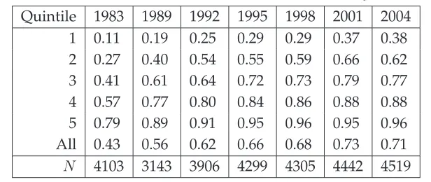
The extensive margin plays a central role in the model as improvements in the lending technology generate an extension of (risky) loans to riskier borrowers. The increase in the number of households with a bank credit card is clear: the fraction of households with a bank credit card jumped from 43% in 1983 to 68% in 1998 (see Table 3). This supports the common narrative of a “democratization of credit” in the 1980s and 1990s.
Table 3: Percent of Households with Bank Credit Card, by Income Quintile
Quintile 1983 1989 1992 1995 1998 2001 2004 1 0.11 0.19 0.25 0.29 0.29 0.37 0.38 2 0.27 0.40 0.54 0.55 0.59 0.66 0.62 3 0.41 0.61 0.64 0.72 0.73 0.79 0.77 4 0.57 0.77 0.80 0.84 0.86 0.88 0.88 5 0.79 0.89 0.91 0.95 0.96 0.95 0.96 All 0.43 0.56 0.62 0.66 0.68 0.73 0.71
N 4103 3143 3906 4299 4305 4442 4519
Source: Survey of Consumer Finances, Bankcards only.
Were the new credit card holders of the 1980s and 1990s risker than the typical credit card holder of the early 1980s? A direct - but rough - proxy for risk is household in-come. Table 3 shows that the rise in card ownership was largest in the middle and lower middle income quintiles, where bank card ownership rose by more than 30 percentage points between 1983 and 1995. This increase in access for lower income households has been accompanied by a significant increase in their share of total credit card debt out-standing. Figure 8(c) plots the cdf for the share of total credit card balances held by various percentiles of the earned income distribution in 1983 and 2004. The fraction of debt held by the bottom 30% (50%) of earners nearly doubled from 6.1% (16.8%) in 1983 to 11.2% (26.6%) in 2004. Given that the value of total credit card debt also increased, this implies that lower income households’ credit card debt increased significantly.39
An alternative approach is to directly examine changes in the risk characteristics of bank credit card holders from 1989 to 1998 in the SCF.40 Since the SCF is a repeated
39The increased access of lower income households to credit card debt is well established, see e.g. Bird,
Hagstrom, and Wild (1999), Fellowes and Mabanta (2007), Lyons (2003), Black and Morgan (1999), Ken-nickell, Starr-McCluer, and Surette (2000), and Durkin (2000).