THE INDONESIAN STOCK MARKET PERFORMANCE DURING ASIAN ECONOMIC CRISIS AND GLOBAL FINANCIAL CRISIS

THE INDONESIAN STOCK MARKET PERFORMANCE DURING ASIAN

ECONOMIC CRISIS AND GLOBAL FINANCIAL CRISIS

MARIA PRAPTININGSIH

Abstract

Volatility in the stock market had strongly affected by the movement of publicly or even inside information. The movements of this information will generate the perspectives and expectations of investors in decision-making. How strong is the level of market efficiency in determining the movement of stock market, especially to achieve stability in the stock market during the economic crisis? How effective are the policies of central banks in controlling the movement of the stock market? This study aims to measure the factors that influence changes in the movement of stock price in Indonesian stock market in terms of market efficiency hypothesis. This research also aims to investigate the effectiveness of central bank policy in controlling and stabilizing the movement of stocks in Indonesia. The research will focus on the economic crisis in 1997 and the global crisis in 2008 as case studies. Thepaperutilizesthe vector error-correction model, impulse responses and variance decomposition in measuring the contribution of the factors that affect the movement of stock and determine the effectiveness of central bank policy. The findings are beneficialto central banks, governments, companies and investors in strengthening the Indonesian Stock Market particularly in facing the threat of financial crisis.

Keywords: efficient market hypothesis, monetary policy, stock market, vector error correction, variance decomposition.

Introduction

The current global financial crisis has affected the economies of countries worldwide, including Indonesia. During the ongoing global economic crisis, it is reported that Asian growth fallen sharply to 1.3 percent in 2009 from 5.1 percent on 2008. (IMF Survey online May 6, 2009). According to the IMF report, that the impact of the global financial crisis particularly on Asia region has been deeper compare to the other region. The most possible reason is many countries in Asia are very dependence on the other region’s economy in terms of their economic integration on export and import activities. Increasingly, it will affect to completely macroeconomic stability in such country, including Indonesia. Therefore, the International Monetary and Financial Committee (IMFC) board was emphasizes on the central role of the Fund in order to help the growth restoration and monitoring the government’s policies that might be taken to solve the crisis. Nowadays, the governments and international organizations are still debating on how national framework on financial and economic stability should change, including the regulation and supervision of financial institution.

Indonesia faced the fallout from the crisis towards the end of 2008, which started on the third quarter. The economic growth was still above 6% with a good performance particular on financial sector. There were some indicators that supported this condition; such as a stable exchange rate, upward moving on stock index, and the declining yield on government securities. Nevertheless, the global financial turbulence started to bear down the Indonesian economy on fourth quarter in 2008. The weakening of exports had pressure the stability on balance of payments and resulted turmoil on the money market as well. The balance of payments began to accumulate a high deficit and depreciation on exchange rate in terms of external side. On the financial markets, there was a rising perception and expectation particular on the country risk because of the global liquidity condition. According to the Indonesian Economic Report (Bank Indonesia, 2008), the Indonesian Stock Market       



and Government Securities prices were fall sharply. The risk spread on Indonesian securities was consider widening and led the foreign capital outflow from the stock market particular in terms of Bank Indonesia Certificates and government securities.

The impact of global crisis was continuing affected Indonesian economy during 2009. Bank Indonesia projects a drop in economic growth around 4.0% along with downside risks if the global economic downturn is greater than expected during 2009. Therefore, the Central Bank of Indonesia (Bank Indonesia) and the Government were concerned to mitigate the impact of this global financial crisis through optimizing monetary and fiscal policies in terms of money sectors and real sectors. It means that the government and Bank Indonesia should have an effective and efficient in coordination and cooperation in order to solve the macroeconomic problems that caused by the global crisis. The following table (Table 1), represents the differences condition in such main macroeconomic indicators between the 1997’s crisis and the current global crisis in terms of Indonesian economy.

As we can see from Table 1, there were significant differences between the impact of 1997 and 2008’s crisis on Indonesian economy. The most powerful indicator to give evidence of Indonesia’s economy falling is GDP. It was 4.7% on 1997 compare with 2008, which is 6.10%. Indonesia’s GDP has gradually declined from 4.7% on 1997 to the lowest level that is -13.7% on 1998 and -10.3% on 1999. This condition was the worst performance on GDP. It was automatically followed by all the main sectors as seen on Table 1. As stated in Yearly Economic Report (1998/1999) by the Central Bank, the pressures on GDP performance occurred when there was a contraction both in aggregate supply and in aggregate demand. On supply side, when the exchange rate was depreciated, therefore the prices of many imported resources in terms of national

Table 1

Indonesia Macroeconomic Condition: Asian Crisis (1997) and Global Crisis (2008)

1997 2008

GDP 4.70% 6.10%

Inflation 11.05% 11.06%

External

- Current Account (% of GDP) -2.30% 0.10%

- International Reserve (billions of USD) 21.40 51.60

- (Month of Imports and Official Foreign Debt Repayment) 5.50 4.00

- Foreign Debt (% of GDP) 62.20% 29.00%

Fiscal

- Fiscal Balance (% PDB) 2.20% 0.10%

- Public Debt (% PDB) 62.20% 32%

Banking

- LDR (%) 111.10% 77.20%

- CAR (%) 9.19% 16.20%

- NPL (5) 8.15% 3.80%

production, increased sharply. This condition pushed up the cost of production as well. Meanwhile, on demand side, the contraction happened when the domestic demand was decrease as well. The main part was on the household consumptions. The decrease on household consumption was caused by the decrease on real income and the level of wealth as well. These are the main impacts of economic crisis on particular period. Similarly, the international reserve indicator had been significantly different between 1997 and 2008. In 1997, it was only 21.4 billions of USD, which had not exceeded than 50% compare to 2008. It was sharply decline because of the high foreign debt and the decline of capital flow as well in the balance of payment. The high percentage of GDP in foreign debt was 62.2% on 1997, while it is only 29% of GDP in 2008. When the economic crisis had happened on 1997, Indonesia was one of the most countries with high debt on particular world organization, such as IMF and World Bank. In 2008, the indicators of external vulnerability in relation to foreign debt showed further improvement, in keeping with the still positive performance of exports.

In stock market, movements of the LQ45 Index and Jakarta Composite Index (JCI) are similar. This means investors also attempt to invest and re-arrange their financial portfolio on Jakarta Composite Index and LQ45 Index in the same manner. The movements in the JCI Index and LQ45 Index had a similar direction but different in the market capitalization. It also implied that investors preferred to invest on the JCI than LQ45 because the JCI moved more actively. During 2003, there was an increase in the price index, volume of trading in the stock market, bond market, and mutual funds. According to Economic Report on Indonesia (2003), this was due to the decline in the interest rate. Moreover, several factors boosted a positive performance on the Indonesian capital market. There were relatively low bank interest rate, improved foreign investors’ perception on Indonesian capital market and relatively stable macroeconomic indicators.1 These were reflected through the increase in Jakarta Composite Index (JCI) in response to the increased stock trading by both domestic and foreign investors. The stock market performance remained bullish in 2004.2 The bullish domestic stock market resulted from continuously improving fundamentals, both in macro and micro contexts, as well as market optimism over the new government. However, the JCI index started to fluctuate, but still generated a positive gain. Internal factors were driving negative sentiment on the stock market including the upward trend in domestic interest rates in consequence to the tight bias monetary policy stance adopted to reduce inflation and depreciation on rupiah. Eventually, the fluctuation on stock market continued until mid of 2008 when the global financial crisis happened.Therefore, this paper will emphasize on investigating whether the monetary policy can have a significant effect on stock market through the monetary policy transmission mechanisms and its indicators.

1. Review of related literature and studies

Efficient market theory is the application of rational expectations to the pricing of securities in financial markets. Current security prices will fully reflect all available information because in an efficient market, all unexploited profit opportunities are eliminated. However, the evidence on efficient markets theory such as market overreaction, excessive volatility on stock prices, and mean reversion condition suggests that the theory may not always be entirely correct. The evidence seems to suggest that efficient markets theory may be a reasonable starting point for evaluating behavior in financial markets but may not be generalizable to all behavior in financial markets. Capital Market plays an important role in the economy of a country because it serves two functions all at once. First, Capital Market serves as an alternative for a company's capital resources. The capital gained from the

      

1

Based on Monetary Policy Transmission Evaluation of Bank Indonesia, Economic Report on Indonesia, 2003, p.67

2

public offering can be used for the company's business development, expansion, and so on. Second, Capital Market serves as an alternative for public investment. People could invest their money according to their preferred returns and risk characteristics of each instrument (Indonesian Stock Exchange Report, 2009). According to Ross (1997); Blanchard, Ariccia, and Mauro (2010), the study empirically proved the existence of a positive relationship between the development of financial systems to economic growth. There are empirical studies that focus on the relationship between monetary policy and financial markets particularly on stock market. Lee (1992) investigated causal relations and dynamic interactions among assets returns, real activity, and inflation in the postwar United States. Major findings are (1) stock returns found to have causality and help explain real activity; (2) stock returns explain little variation in inflation, although interest rates explain a substantial fraction of the variation in inflation; and (3) inflation explains little variation in real activity. Based on these findings, many researchers developed new research and studies in terms of financial markets, particularly on monetary policy effect toward the financial market [e.g. Thorbecke (1997), Rigobon and Sack (2003), and Gupta (2006)]. Thorbecke (1997) examined how stock return data respond to monetary policy shocks. The evidence states that monetary policy exerts large effects on ex-ante and ex-post stock returns. The macroeconomic indicators can affect the stock price movement. Similarly, Rigobon and Sack (2003) investigated the relationship between monetary policy and financial market. In addition, they proved that movements in the stock market can have a significant impact on the macro-economy and are therefore likely to be an important factor in the determination of monetary policy. The results suggest that stock market movements have a significant impact on short-terms interest rates, driving them in the same direction as the change in stock prices. Similarly, Bernanke &Gertler (2000) concluded that in order to explore the issue of how monetary policy should respond to variability in asset prices particularly in stock market, the paper incorporated non-fundamental movements in asset prices into a dynamic macroeconomic framework. It is necessary for monetary policy to respond to changes in asset prices.

There are several empirical evidences that utilized the vector error correction approach in examining the effect of monetary policy to macroeconomic indicators and stock market. Granger (1986); Johansen and Juselius (1990) examined the existence of long term equilibrium among selected variables by utilizing the cointegration analysis. A cointegration happened when a set of time series data were found to be stationary or they had a same order in linear combination. This linear combination shows that they have a long-term relationship between the variables. The main advantage of cointegration analysis is that through an error correction model (ECM), the dynamic co-movement among variables and the adjustment process toward long-term equilibrium can be examined (Maysami, 2004). Mukherjee and Naka (1995) examined the relationship between Japanese Stock Market and exchange rate, inflation, money supply, real economic activity, long-term government bond rate, and call money rate. They applied VECM to test a cointegration. The results found that there is a cointegrating relationship and stock prices had contributed to the variables. Maysami and Koh (2000) applied the similar topic and methodology in Singapore. Meanwhile, the VEC approach is employed to examine the impact and relationship between stock returns and macroeconomic variables in Hong Kong and Singapore (Maysami and Sim, 2002b), Malaysia and Thailand (Maysami and Sim, 2001a), and Japan and Korea (Maysami and Sim, 2001b). Vuyyuri (2005) used similar methodology to investigate the cointegrating and causality between the financial and the real sectors of the Indian economy from 1992 to 2002 in monthly data. Therefore, this study will extend the literatures through utilizing Johansen’s (1988) results to investigate the relationship between monetary variables and stock market indices in the long-run equilibrium.

2. Research hypothesis and methodology

Composite Index (JCI), and LQ45 Index. Nevertheless, in order to get additional data to sharpen the analysis, this paper also optimizes the Central Bank Annual Reports, The IMF Reports, World Economic Outlook Database by IMF, and other sources of data.

Co-integration states that if the time series data are not stationary or has a unit root, the combination of two or more of time series variable will form a linear combination that contain a co-movement, assuming there is no deviation in the long term. The paper utilizes the Johansen Cointegration Test to check whether the variables have cointegrating relationship if the variables are found to be non-stationary or I(1), I(2). This cointegrating analysis represents a short-term dynamics of the variables. Impulse responses serve to test the response of each variable in the current period and in the future by assuming that the error of other variables is zero (Stock & Watson, 2007). Stock & Watson (2007) defined that forecast error decomposition is the percentage of the variance of the error made in forecasting a variable due to a specific shock at a given horizon. According to Enders (2004), the forecast error variance decomposition tells us the proportion of the movements in a sequence due to its “own” shocks versus shocks to the other variable. The following are the models:

Where JCI is the Jakarta Composite Index at time t; LQ45 is the most forty-five liquid stocks in Indonesia Stock Exchange at time t; BI is the Bank Indonesia Rate at time t; α is a constant and is an error term. Time t is in quarterly and j is lagged values that are chosen by the best estimation.

3. Results and analysis

The paper found that for the BI rate, since the computed ADF test statistics (-2.028922) was greater than the critical values (-3.474265, -2.880722 and -2.577077 at 1%, 5% and 10% significant level, respectively), the result could not conclude to reject null hypothesis (H0). That means the BI

rate series has a unit root problem. It means the BI rate series is a non stationary series. Similar results were also found for Jakarta Composite Index (JCI) and LQ45. All these variables are non stationary at level I(0). Therefore, the paper attempted to transform the time series data from non-stationary to non-stationary, since the estimation required a non-stationary time series data. All the variables were transformed into first difference or I(1). The paper found that for the BI rate, the absolute computed ADF test statistic (-6.120027) is smaller than the critical values (-3.474265, -2.880722 and -2.577077)and the result concluded that the null hypothesis (H0) was rejected. That means the BI rate

does not have a unit root problem and the BI rate series is stationary at first difference. Similar results also happened to the Jakarta Composite Index (JCI) and LQ45. In general, the paper concludes that all six variables are stationary at first difference or I(1). Thus, this requires the cointegration method to be conducted.

theory. Nevertheless, this model is restricted to the dynamic changes that might be occurring on the observation. Hence, the Granger Causality is employed to test the predictability among variables. Table 2 presents several variables that are statistically significant at various levels, which are 1%, 5%, and 10%. The results confirmed that Jakarta Composite Index (JCI) and LQ45could help in predicting the movement in the BI rate. Meanwhile, the Jakarta Composite Index (JCI) could help in predicting LQ45. The following is the summary result of Granger Causality Test:

Table 2

Pairwise Granger Causality Tests

Null Hypothesis: Obs F-Statistic Probability

LN_JCI does not Granger Cause LN_BI_RATE 150 4.28362 0.01558

LN_BI_RATE does not Granger Cause LN_JCI 1.68583 0.18890

LN_LQ45 does not Granger Cause LN_BI_RATE 150 3.81558 0.02427

LN_BI_RATE does not Granger Cause LN_LQ45 1.24940 0.28974

LN_LQ45 does not Granger Cause LN_JCI 150 0.15893 0.85320

LN_JCI does not Granger Cause LN_LQ45 8.83723 0.00024

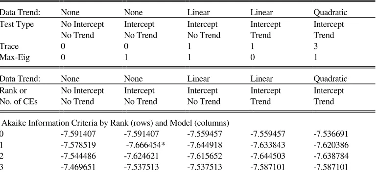
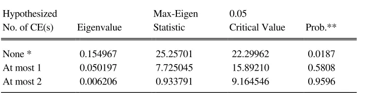
Table 3provides the Johansen Co-integration summary results.The model without intercept and trends is the best assumption chosen by the lowest value of AIC criterion. The minimum requirement for at least one co-integration was confirmed based on the result. Table 4 presents the max-eigenvalue test which provides one cointegrating equation at 0.05 levels. Thus, it may be concluded that there isonecointegrating vectors found in the series of variables at 0.05 confidence level.

Table 3

Johansen Cointegration Test Summary

Selected (0.05 level*) Number of Cointegrating Relations by Model

Data Trend: None None Linear Linear Quadratic

Test Type No Intercept Intercept Intercept Intercept Intercept

No Trend No Trend No Trend Trend Trend

Trace 0 0 1 1 3

Max-Eig 0 1 1 0 1

Data Trend: None None Linear Linear Quadratic

Rank or No Intercept Intercept Intercept Intercept Intercept

No. of CEs No Trend No Trend No Trend Trend Trend

Akaike Information Criteria by Rank (rows) and Model (columns)

0 -7.591407 -7.591407 -7.559457 -7.559457 -7.536691

1 -7.578519 -7.666454* -7.644918 -7.633843 -7.620386

2 -7.544486 -7.624621 -7.615652 -7.644503 -7.638784

Table 4

Johansen Cointegration Test Unrestricted Cointegration Rank Test (Maximum Eigenvalue)

Hypothesized Max-Eigen 0.05

No. of CE(s) Eigenvalue Statistic Critical Value Prob.**

None * 0.154967 25.25701 22.29962 0.0187

At most 1 0.050197 7.725045 15.89210 0.5808

At most 2 0.006206 0.933791 9.164546 0.9596

Max-eigenvalue test indicates 1 cointegratingeqn(s) at the 0.05 level

Table 5 Speed of Adjustment Parameter of the Error Correction Term (ECT)

Standard errors in ( ) & t-statistics in [ ]

Error Correction:

D(LN_BI_RAT

E) D(LN_JCI) D(LN_LQ45)

CointEq1 -0.000833 0.003010 0.019855

(0.00600) (0.00766) (0.00893) [-0.13883] [ 0.39283] [ 2.22363]

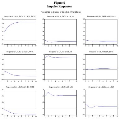
Figure 6

Response of LN_BI_RAT E to LN_BI_RAT E

-.04

Response of LN_BI_RAT E to LN_JCI

-.04

Response of LN_BI_RAT E to LN_LQ45

-.08

Response of LN_JCI to LN_BI_RAT E

-.08

Response of LN_LQ45 to LN_BI_RAT E

-.05

Response to Cholesky One S.D. Innovations

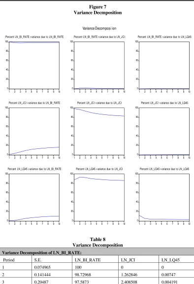
Figure 7

Percent LN_BI_RATE v ariance due to LN_BI_RATE

0

Percent LN_BI_RATE v ariance due to LN_JCI

0

Percent LN_BI_RATE v ariance due to LN_LQ45

0

Percent LN_JCI v ariance due to LN_BI_RATE

0

Percent LN_JCI v ariance due to LN_JCI

0

Percent LN_JCI v ariance due to LN_LQ45

0

Percent LN_LQ45 v ariance due to LN_BI_RATE

0

Percent LN_LQ45 v ariance due to LN_JCI

0

Percent LN_LQ45 v ariance due to LN_LQ45

Variance Decomposi ion

Table 8

Variance Decomposition

Variance Decomposition of LN_BI_RATE:

Period S.E. LN_BI_RATE LN_JCI LN_LQ45

1 0.074965 100 0 0

2 0.141444 98.72968 1.262846 0.00747

4 0.26338 96.8602 3.13702 0.002777

5 0.316776 96.40912 3.586235 0.004645

6 0.365464 96.13138 3.859255 0.009361

7 0.410045 95.95829 4.025496 0.016218

8 0.451116 95.8498 4.125889 0.024306

9 0.48921 95.78143 4.185613 0.032961

10 0.52478 95.73835 4.219972 0.041673

Average 0.324205 96.904555 3.0810834 0.0143602

Variance Decomposition of LN_JCI:

Period S.E. LN_BI_RATE LN_JCI LN_LQ45

1 0.095784 1.695133 98.30487 0

2 0.14836 3.593436 96.40608 0.000482

3 0.19057 5.29633 94.69188 0.011792

4 0.226333 6.68833 93.28129 0.030378

5 0.257787 7.784221 92.15754 0.058239

6 0.285989 8.642386 91.26849 0.089125

7 0.311682 9.316735 90.56161 0.12166

8 0.335363 9.852105 89.99419 0.153704

9 0.357409 10.28221 89.53338 0.18441

10 0.378098 10.6323 89.15456 0.213137

Average 0.2587375 7.3783186 92.535389 0.0862927

Variance Decomposition of LN LQ45:

Period S.E. LN BI RATE LN JCI LN LQ45

1 0.111613 0.424571 86.53372 13.04171

2 0.17369 1.559146 92.33948 6.101375

3 0.217048 2.696856 92.87756 4.42558

4 0.252922 3.682911 92.98074 3.336348

5 0.282976 4.495369 92.81698 2.687655

6 0.309396 5.143824 92.60772 2.248453

7 0.332985 5.661842 92.3943 1.94386

8 0.354488 6.076156 92.19799 1.725851

9 0.374338 6.411111 92.02339 1.565496

10 0.392878 6.684782 91.87029 1.444927

Average 0.2802334 4.2836568 91.864217 3.8521255

values by 92.5353 percent, 7.3783 percent of BI rate, and 0.0862 percent of LQ45. Third is the variance of LQ45 which is mainly affected by its lagged values of 3.8521 percent, followed by 4.2836 percent of BI rate, and 91.8642 percent from JCI.

Conclusions

The paper concludes that monetary policy is effective in achieving the financial markets stability through each indicator. Findings are consistent with the hypothesis that the monetary instruments have a significant effect in achieving the improvement particularly on stock market index. Bank Indonesia had utilized all the monetary instruments effectively through the monetary policy transmission mechanisms. The effectiveness of monetary instruments, that is Bank Indonesia rate generates market expectations toward the credibility of the policy makers. In addition, there is a positive expectation of investors and firms toward the macroeconomic performance. Therefore, Bank Indonesia as the monetary authority played an important role in straightening up the linkage between financial and monetary policy. The paper recommends Bank Indonesia to use the overnight interbank money market rate as the monetary policy operational target. The evidence proved that 1-month BI rate is effective in affecting the JCI by 7.3783 percent.Meanwhile,1-month BI rate is effective in affecting LQ45 by 4.2836 percent.

Moreover, the paper also recommends Bank Indonesia in reducing the lag effect, which is two quarter particularly in the stock market. By reducing the lag effect, it can reduce the overreaction of the investors. Thus, Bank Indonesia would be effective in controlling the stock market movement. Bank Indonesia should encourage investors to invest in real sectors. Buying stocks of real sector companies such as manufacturing can generate high capital inflows toward the industries. Thus, it can lead to high production capacity and aggregate output. The objective of the monetary policy is to control and boost up the foreign investment through stock market.

Thus, it will achieve a steady economic growth. In order to generate a high economic growth through the changes in monetary policy instruments such as money supply and the interest rates, Bank Indonesia should respond carefully, regarding the trade-off phenomenon between price stability and economic growth.

References

 Baltagi, B.H., 2003, “A Companion to Theoritical Econometrics”, Blackwell Publishing

 Baltagi, B.H., 2008,“ Econometric Analysis of Panel Data”, Third Edition, John Wiley & Sons Ltd.

 Bank Indonesia, 2008, Indonesian Economic Report, Bank Indonesia

 Bernanke, B. and Gertler, M., 2000, “Monetary Policy and Assets Price Volatility”, NBER Working Paper No. 7559, February 2000

 Bernanke, B.S., 2008, Macroeconomics, Sixth Edition, Pearson Addison-Wesley

 Blancard, O.J., Ariccia, G.D., and Mauro, P., 2010, “Rethinking Macroeconomic Policy”, IMF Staff Position Notes SPN/10/03

 Cargill, T.F., 1991, Money, The Financial Systems, and Monetary Policy, Fourth Edition, Prentice-Hall International Editions

 Enders, W., 2004, Applied Econometric Time Series, Second Edition, Wiley

 Ferguson Jr, R.W., (2003) “Monetary Stability, Financial Stability and the Business Cycle: Five Views”,

Bank for International Settlements Papers, No.18, Monetary and Economic Department, September 2003, p.7-15

 Fraga, A., Goldfajn, I., and Minella, A., 2003, “Inflation Targeting in Emerging Market Economies”, NBER Macroeconomics Annual, Vol. 18, pp 365-400, The University of Chicago Press

 Greene, W.H.,2003. “Econometric Analysis”, Fifth Edition, Prentice Hall

 Indonesia Stock Exchange Website: www.idx.co.id

 Issing, O., (2003), “Monetary Stability, Financial Stability and the Business Cycle: Five Views”, Bank for International Settlements Papers, No.18, Monetary and Economic Department, September 2003, p.16-23  Johansen, S. and Juselius, K. 1990, “Maximum Likelihood Estimation and Inference on Cointegration with

Application to the Demand for Money”. Oxford Bulletin of Economics and Statistics 52:169-210

 Kasa, K. 1992, “Common Stochastic Trends in International Stock Markets”, Journal of Monetary

Economics, 29: 95-124.

 Lutkepohl, H., 2003, “Vector Autoregressions”, Blackwell Publishing

 Mishkin, F.S., and Eakins, S.G., 2000, Financial Markets and Institutions, Third Edition, Addison-Wesley

 Pesaran, M.H., and Wickens, M., 1995, Handbook of Applied Econometrics, Macroeconomics, Blackwell Publishing.

 Rigobon, R., and Sack, B. 2003, “Measuring the Reaction of Monetary Policy to the Stock Market”, The Quarterly Journal of Economics,Vol 118, No.2, pp. 639-669

 Romer, D., 2006, Advanced Macroeconomics, Third Edition, McGraw-Hill

 Ross, L. 1997, “Financial Development and Economic Growth: Views and Agenda”, Journal of Economic Literature, Vol. 35 (2)

 Serletis, A. and King, M. 1997, “Common Stochastic Trends and Convergence of European Union Stock Markets”, The Manchester School, 65(1): 44-57.

 Stock, J.H., and Watson, M.W., 2001, “Vector Autoregressions”, Journal of Business and Economic Statistics, pp. 1-28.

 Taylor, J.B., 1993, “The Use of the New Macroeconometrics for Policy Formulation”, The American Economic Review, Vol.83, No.2, pp. 300-305

 Thomas, L.B., 1997, Money, Banking, and Financial Markets, Irwin-McGraw-Hill

 Thorbecke, W., 1997, “On Stock Market Returns and Monetary Policy”, The Journal of Finance, Vol.52, No.2, pp. 635-654

 Valadkhani, A., 2003, “History of MacroeconometricModelling: Lessons From Past Experience”,

Discussion Papers in Economics, Finance and International Competitivenes, School of Economics and

Finance, Queensland University of Technology