THE IMPACT OF MONETARY POLICY TOWARD INDONESIAN STOCK MARKET UNDER INFLATION TARGETING REGIME

(1)

240

Lex ET Scientia. Economics Series

THE IMPACT OF MONETARY POLICY TOWARD

INDONESIAN STOCK MARKET UNDER INFLATION

TARGETING REGIME

Maria PRAPTININGSIH*

Abstract

A high volatility in stock market movement can be influenced by current news both domestic and international economic shocks, including the ongoing global financial crisis that affect Indonesian economy in particular. Based on empirical studies and theories, that monetary policy can be an effective tool in order to stabilize the stock market volatility. Monetary policy can have a significant effect on the movement in stock market. Does it really happen on Indonesian macro economy? This paper investigates the relations between monetary policy by its instruments and stock market movement. Our empirical evidence is based on before and after the adoption of Inflation Targeting Framework, including the period of Asian Crisis (1997) and the Global Financial Crisis (2008). This paper uses a Vector Error Correction Model (VECM) in order to examine the dynamic movement and changes on Indonesian Stock Market as an impact of the changes in monetary policy in terms of Inflation Targeting regime. Utilizing an Impulse Response and Variance Decomposition approach, this paper analyzes the effectiveness of monetary policy toward the stock market performance in order to achieve the stability of stock market and to develop market expectations. These objectives are beneficial to strengthen the credibility of the Central Bank as the monetary authority in terms of the implementation of Inflation Targeting Framework. Furthermore, this paper attempt to assess and evaluate the monetary policy and induce the central bank to create an optimal policy in the future.

Keywords: inflation targeting framework, monetary policy, stock market, vector error correction, variance decomposition

1. Introduction

Stock market has become one of the main subjects in terms of macroeconomic stability. Since the monetary policy has, an objective to achieve the price stability in terms macro economy, therefore the stance of the Central Bank whereas the monetary authority is needed to influence the stock market particularly. Movements in the stock market can have a significant impact on the macro-economy.1 Reversely, the change in macroeconomic variables can have a significant impact as well on the movements in the stock market. These relationships will have a significant result in order to provide comprehensive information to the policy makers to respond and create optimal policy in terms of macroeconomic stabilization.

Nevertheless, it is still difficult to identify the monetary policy response to the stock market. However, based on the theory that the monetary policy can influence the stock market by its instruments, such as the interest rates, therefore, we would like to emphasize on the stock market

*

Department of Business Management, Faculty of Economics, Petra Christian University, Surabaya, Indonesia (e-mail: maria_npa@yahoo.com)

1

(2)

response to the change on macroeconomic variables. These variables will represent the stance of monetary policy in terms of inflation targeting framework. The adoption of inflation targeting framework based on the objectives of the Central Bank to achieve the price and macro-economy stabilities, through setting the range of inflation target.

According to the Bank Indonesia Yearly Report2, stated that during the Asian Crisis on 1997 to 2000, the foreign investors tend to implement only hit and run trade strategies. It means that the investors attempt to boost their gain only on a very short time. Meanwhile, the similar situation had happened on money market. This condition pushed the investors more un-sensitive regarding the change of interest rates. In terms of high country risk, the difference between domestic and international interest rates might not be the only main reasons for investors to change their portfolios. In fact, there were several arguments that investors had change their portfolio from Indonesian capital market to other countries.3 First, there was a profit motive, regarding the high interest rate on other capital market particular on United States of America. Second, it was called flight to quality motive. The motive occurred in order to maintain their portfolio because of the downward performance on emerging market particularly. These two particular factors were indirectly became barrier to the portfolio investment and capital inflow to Indonesian financial market.

Increasingly, the central bank started to implement some policies in order to improve the performance of capital market, namely the regulation on stock pricing. However, this particular policy was un-sufficient to boost up the capital market performance. Moreover, the downturn performance of capital market remains until 2002. At the end of 2001, the Composite Index was 5.83% decreased from 416.3 to 392.0 levels. It was mainly affected by the depreciation on rupiah; the increase on Bank Indonesia rate to 17%; and the downgrade of investment rating in Indonesia, from “stable” to “negative” based on Moody’s on March 2001.4 Furthermore, these circumstances even worst when the government raised the tax policy particular on bond return to 0.003%. This policy was contra-productive in terms of improving the capital market performance as one of the financing institution.

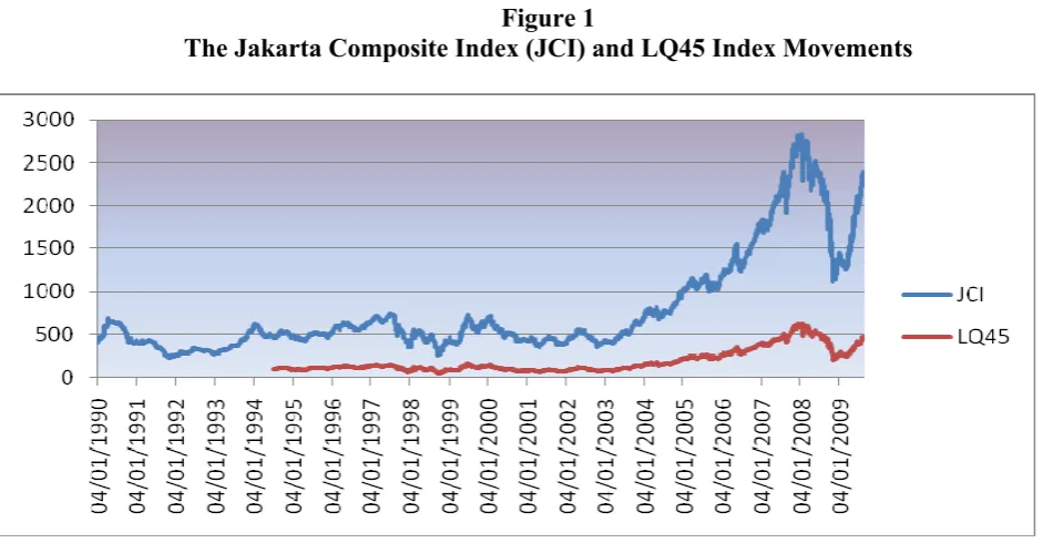
In addition, we can analyze the stock market fluctuation in detail from the following figures.5 There are the movements of Jakarta Composite Index (from 1990 to 2009) as well as the LQ45 index (from 1994 to 2009), given as follows:

2

Indonesian Economic Report 1997, p. 64; 1998, p.70; 1999, p.72; 2000, p.75; Macroeconomic and Monetary Condition

3

Based on the survey of Bank Indonesia and Indonesian Capital Market and Financial Institution Supervisory Agency, 1999

4

Based on the Financial Market Report, Economic Report on Indonesia, Bank Indonesia, 2001

5

(3)

242

Figure 1

The Jakarta Composite Index (JCI) and LQ45 Index Movements

Source: Bloomberg, 2010

According to figure 1 above, we can see that the similar movement are happened on LQ45 Index as on Jakarta Composite Index (JCI). The LQ45 index is the index of forty-five stocks that most liquid and have the highest market capitalization. It means that investors also attempt to invest and re-arrange their financial portfolio on Jakarta Composite Index as well as LQ45 Index.

During 2003, there was an increase on price index, volume of trading in the stock market, bond market, and mutual funds. This was affected by the decline in the interest rate. Several factors had boosting the positive performance of Indonesian capital market.6 There were: (1) relatively low bank interest rate, which enable the investor to gain higher profit on capital market instead of bank deposits; (2) improved foreign investors’ perception on Indonesian capital market as well as the country risk and a significant difference on interest rate that cause high capital inflows to gain short-term profits; (3) relatively stable on macroeconomic indicators. This was reflected by increased Jakarta Composite Index (JCI) in response to increased stock trading both by domestic and foreign investors. The JCI closed at level 691.9 and increased up by 266.9. This increased JCI gained a profit of 62.8% compared the position at end 2002. Positive performance also occurred upon LQ45 index, which increased 59.9 to 151.9 in 2003 compared to previous year. The improved JCI and LQ45 performance was related to several international stock exchanges positive performance and relatively low bank interest rate.

The stock market performance was remained bullish on 2004.7 The continuing trends as on 2003 pushed the composite index above the 1,000 level before year-end. The bullish domestic stock market resulted from continuously improving fundamentals, both in macro and micro contexts, as well as market optimism over the new government. The upward trend continued during 2005. However, the JCI index started to fluctuate, even still a positive gain. Internal factors were driving negative sentiment on the stock market included the upward trend in domestic interest rates in consequence to the tight bias monetary policy stance adopted to reduce inflation

6

(4)

and depreciation on rupiah. The other factors that bearing down on the JCI were the surge in world oil prices to almost $70 per barrel.8 The market had negative projections on the performance the stock markets. Moreover, it also induced by the raised on the domestic interest rates regarding the tight monetary policy stance. Eventually, the fluctuation on stock market continued until year-mid on 2008, when the global financial crisis had happened. The Composite Index closed at 1,355 at the end of 2008, a drop of 50.64% compared to the previous year. At the beginning of 2008, the index was relatively impressive. It was 2,830 level which was the highest level ever recorded since the beginning of Indonesia Stock Exchange.

Furthermore, Bank Indonesia attempted to minimize the negative impact of any economic shocks that can dropped financial markets performance as well as the macro stability. Therefore, the policies of Bank Indonesia, which is represent by the Indonesian Capital Market and Financial Institution Supervisory Agency and the Indonesian Stock Exchange Board are plays an important role in limiting a deeper financial markets decline, particular on Composite Index.

According to the consequence of monetary policy stance toward the financial markets performance through the financial systems mechanisms, then we provide a brief summary of several macroeconomic performances in terms of particular indicators, as follows:

Table 1.

Selected Macreconomic Indicators9

Percent

Description 2003 2004 2005 2006 2007 2008

GDP Growth 4.7 5.0 5.7 5.5 6.3 6.1

CPI Inflation 5.1 6.4 17.1 6.6 6.6 11.0

Core Inflation 6.9 6.7 9.8 6.0 6.3 8.3

Average Exchange Rate (Rp/$) 8,572.0 8,940.0 9,713.0 9,167.0 9,140.0 9,241.0 SBI (1 month)/BI Rate since July

2005 8.3 7.4 12.8 9.8 8.0 8.6

Current Account/GDP 3.4 0.6 0.1 2.9 2.5 0.1

Sources: BPS-Statistic Indonesia; Bank Indonesia

In 2005, CPI inflation rose gradually to 17.1%, following the October hikes in fuel prices. The shocks in this index was primarily driven by fuel prices and other administered prices, in particular transportation tariffs. Higher inflation expectations and rupiah depreciation also raised core inflation while downward pressure from the output gap remained relatively insignificant. Against the backdrop, CPI inflation was above the determined target of 6%+/-1% for 2005. The core inflation rate was high in 2005, peaking at 9.7%, primarily attributable to high inflationary expectations and depreciating exchange rates. Higher inflationary expectations from the public were visible as Q1-2005 closely associated with the government’s plan to adjust domestic fuel prices in line with global oil prices and weaker exchange rates.

The rise in the Bank Indonesia (BI) rate, that is, an anchor for the interest rate determination in Indonesia, and deposit rate was followed by a limited increase in lending rate, whereas the

8

Based on International Economic Evaluation, Economic Report on Indonesia, 2004, p.70

9

(5)

244

volume of credit allocation remained relatively high. The lending rate began to increase during October 2005 to 15.18% from 13.41% at the end of 2004. This verified that the role of banks in financing the economy remains imperative. In brief, the rise in the BI Rate has not negatively affected bank intermediation. In order to reduce inflation and restore monetary stability, Bank Indonesia tightened further its monetary policy, primarily through the implementation of a new Inflation Targeting Framework (ITF) supplemented by exchange rate stabilization packages.10

Eventually therefore, this study will emphasize on two basic research questions, which is based on the background that discussed earlier. The first is to examine whether the monetary policy can have a significant effect in order to achieve its objectives in terms of the inflation-targeting framework. The purpose of this particular problem is to measure the credibility of Bank Indonesia regarding the basic requirements of the inflation-targeting implementation, namely credibility, transparency, and accountability. The second is to investigate whether the monetary policy can have a significant effect on financial markets, particular on stock market. The result will be beneficial to the market players in terms of their decision-making regarding the market perception and expectation. In conclusion, the study will provide a valuable knowledge and experience based on the empirical studies and current research in terms of monetary policy and financial systems.

2. Review of related literature and studies

2.1.The Definitions and Concepts of Inflation Targeting

There are many definitions and concepts within the inflation targeting, which need to be verified before proceeding to the next section. These definitions and concepts arise from the way of conducting inflation targeting policies. Green (1996) define inflation targeting is a framework for conducting monetary policy in which decisions are guided by expectations of future inflation relative to the announced target. In inflation –targeting setup, the authorities announce a target or, more typically, a target range for future inflation. The change in the policy reaction is represent of the change in the projected inflation over one to two-year time horizon in terms of decreasing from the announced band of inflation target. Therefore, later the expected future inflation called an intermediate target as the monetary authorities used it into the monetary policy indicators. Meanwhile, Romer (2006) define that inflation targeting does not mean a single-minded focus on controlling inflation. Instead, there are three basic indicators that inflation targeting working on. First, which is becomes the main part that there is an explicit target for inflation. The target is typically quite low and usually specified as a range or in interval of a few percentage points. Second, central banks in inflation-targeting countries (inflation targeters) appear to have more weight than other central banks on conducting the inflation. Lastly, there is greater emphasis on making the central bank’s policies transparent and central bankers accountable for the policies.

There are two main concepts that are use as a basic reference for this study, which are implicit vs. explicit inflation targeting and strict vs. flexible inflation targeting. The first concept is implicit vs. explicit inflation targeting. Hammour (2005) define an implicit inflation targeting implies that the monetary authority does not have to pre-announce and report publicly its inflation target. As an example on this type is the current monetary policy in the United States. The Central bank of United States (The Fed) controlling and maintain the inflation rate and other macroeconomic indicators, and then reacts at the first sign of inflation or excess demand by changing its instrument such as the interest rate upward. In other condition, explicit inflation targeting requires pre-announcement of inflation targets and reporting periodically to the public

(6)

the developments in the monetary policy and the success or the failure to achieve the targets. Therefore, explicit inflation targeting implies full accountability and transparency of monetary policy. According to this differentiation, the inflation-targeting concept used in this study is meant to be the explicit type.

The second concept that we describe is what Svensson refers to, in many papers (1997a, 1997b, and 1998) and in Rudebusch and Svensson (1998), as strict versus flexible inflation targeting. Ball (1997) describes those two types as narrow versus broad definitions respectively. First, strict inflation targeting is a single-target policy where the central bank’s objective function contains only inflation. In other point of view, the flexible inflation targeting is a multi-target regime where the monetary authority includes more than inflation in its objective function, such as the real output and interest rate. The first type implies that the central bank has to set its instruments in such a way that the target is met every period. This type of policy would lead to more variability and fluctuations in the output and interest rate. Therefore, the adjustment under flexible inflation targeting is slower or gradual as compared to the strict type.

Furthermore, Romer (2006) stated that there are two main views of inflation targeting. The first is that it is merely “conservative window-dressing”. In this view, the important changes in monetary policy are that the central bank has decided to aim for lower inflation than in earlier decades and to put greater emphasis on the behavior of inflation. The other features of inflation targeting, such as the formal targets, inflation reports, and so on, are of little importance. The other view is that inflation targeting matters. This view focuses on credibility, transparency, and accountability. Discussions of credibility argue that the emphasis on hitting the inflation target can affect expected inflation. This can be important in two situations. The first is when inflation targeting is adopted. Typically, this is done when inflation is well above the newly adopted target. Thus, inflation targeting may reduce expected inflation, and hence lower the output costs of the disinflation needed to get inflation down to the target. This idea is appealing and plausible. The second situation is where the disturbances move inflation away from the target. By anchoring expectations at the target level, inflation targeting can reduce the disturbance’s impact on expected inflation. Indeed, there is some evidence that shocks to the price level have little influence on expected inflation under inflation targeting. Since disturbances are both positive and negative, this is not likely to have a large effect on average output. Nevertheless, it can make the economy more stable.

In many literatures, we found that inflation targeting has both several advantages and disadvantages during a certain period of research. Based on these findings, it will provide a reference as a basic argument in order to examine the effectiveness of inflation-targeting framework. Accordingly, this study will describe both advantages and disadvantages of inflation targeting taken from particular research.

The first is the advantages of inflation targeting which as a medium-term strategy for monetary policy (Mishkin, 2001). In contrast to an exchange rate peg, inflation targeting enables monetary policy to focus on domestic considerations and to respond to shocks to the domestic economy. In contrast to monetary targeting, another possible monetary policy strategy, inflation targeting has the advantage that a stable relationship between money and inflation is not critical to its success: the strategy does not depend on such a relationship, but instead uses all available information to determine the best settings for the instruments of monetary policy. Inflation targeting also has the key advantage that it is easily understood by the public and thus highly transparent.

(7)

246

instability. Forth, that it will lower economic growth. Fifth, that inflation targeting can only produce weak central bank accountability because inflation is hard to control and because there are long lags from the monetary policy instruments to the inflation outcome, is an especially serious one for emerging market countries. Sixth, that inflation targeting cannot prevent fiscal dominance. Lastly, that the exchange rate flexibility required by inflation targeting might cause financial instability, are also very relevant in the emerging market country context.

There are many studies discussed inflation targeting. Study of Green (1996) and Smith (2005) focused on the theory of inflation targeting and core inflation as well, and the policy implication to the economy. Green’s findings are inflation targeting can be classified either as a rule or as discretionary. The literature identifies an inherent bias that on average causes inflation to exceed the socially preferred level. This bias is sometimes offered as an explanation for higher than desirable inflation rates. However, in setting the low-inflation target, an apparent inconsistency is introduced: average and expected inflation will exceed the announced inflation target. Meanwhile, Smith (2005) found that both the level of accommodation of the central bank and the inflation expectations of agents affect, which measure is core inflation. From the conditional results, there are no changes in the public’s beliefs about the regimes. Hence, all regimes would be ranked equivalently. Moreover, the gain from inflation targeting lies in the fact that it makes central banks less accommodative but not in making, the public believe that the central bank is less accommodative.

Therefore, in order to deliver the outcomes of inflation targeting, such as control the inflation rate, raise output growth, lower unemployment, and increase external competitiveness, there must exists a strong institutional commitment to make price stability as the primary goal of the central bank.

2.2.The Role of the Central Bank on Inflation Targeting Framework

The Central Bank has a main role to conduct the Inflation Targeting Framework. Mishkin (2001) stated that inflation targeting is a recent monetary policy strategy that encompasses five main elements: (1) the public announcement of medium-term numerical targets for inflation; (2) an institutional commitment to price stability as the primary goal of monetary policy, to which other goals are subordinated; (3) an information inclusive strategy in which many variables, and not just monetary aggregates or the exchange rate, are used for deciding the setting of policy instruments; (4) increased transparency of the monetary policy strategy through communication with the public and the markets about the plans, objectives, and decisions of the monetary authorities; and (5) increased accountability and credibility of the central bank for attaining its inflation objectives. Nevertheless, the crucial point about inflation targeting is much more than a public announcement of numerical targets for inflation for the year ahead. There are at least three major challenges that the monetary authorities, here the central bank and government, faces: (1) building credibility; (2) reducing the level of inflation; and (3) dealing with the fiscal, financial, and external dominance (Fraga, 2003).

The adoption of inflation targeting represents an effort to enhance the credibility of the monetary authority as committed to price stability. The fact is that building credibility takes time. The central bank’s policies not only have to be consistent with the inflation-targeting framework, but they also have to take into account that private agents do not fully trust that the central bank will act accordingly. Moreover, private agents have concerns about the commitment of the central bank to the target itself and to its reaction to shocks.

(8)

and well-defined inflation target can be instrumental in building support for an independent central bank, even in the absence of a rigidly defined and legalistic standard of performance evaluation and punishment (Mishkin, 2001).

As illustrated in Mishkin and Posen (1997), and in Bernanke (1999), inflation-targeting central banks have frequent communications with the government, and their officials take every opportunity to make public speeches on their monetary policy strategy. Inflation-targeting central banks have taken public outreach a step further that is an Inflation Report-type document to clearly present their views about the past and future performance of inflation and monetary policy. Therefore, each central bank and government in such a country that adopts inflation targeting should maintain and cooperate in effective and efficient policies.

Recent empirical studies provide evidence that independent central banks foster lower and less volatile inflation rates but do not appear to produce lower or more volatile output. Based on this evidence, some authors have concluded that central bank independence is a “free lunch” that delivers price stability without apparent real output costs. This approach is questionable given that many countries did not establish independent central banks. Some explanation rests on the existence of a credibility versus flexibility trade-off associated with the setting up of an independent central bank. Study of Lohman (1992) and Cukierman (1994) were developed models where the central bank independence originates a trade-off between the credibility gains associated with central bank independence and the flexibility costs arising from a suboptimal stabilization policy.

In terms of case study research, there are Kannan (1999); Chowdury & Siregar (2004); Fraga, Goldfajn, & Minella (2003); and Johnson (2003) that focused on the implementation of inflation targeting on many countries. Kannan (1999) describe the inflation targeting implementation in India. This study found that in India, stipulated annual variation in broad money is considered as an intermediate target under the monetary targeting framework and its act as a domestic anchor for monetary policy with feedback. In the April 1998, monetary policy a move towards indicators approach was announced, where the RBI takes into account the developments in a host of macroeconomic indicators such as money, credit, prices, etc, in the conduct of its monetary policy.

Study of Chowdury & Siregar (2004) focuses on Indonesia’s monetary dilemma, which is the constraint of inflation targeting. The result stated that the essence of inflation targeting is embedded in the so-called social welfare function that includes both inflation and economic growth. When the relationship is found to be positive in the short run or at the moderate rate of inflation, the society has to weigh the cost of low inflation vis-à-vis cost of lost output. In the context of Indonesian transition, one has to evaluate the risk of a prolonged recession for democratic consolidation and social conflict. It is affected by the danger of higher inflation and its likely negative effect on output.

(9)

248

2.3.Monetary Policy Implication from Inflation Targeting

The single objective of Indonesian monetary policy is to maintain the stability in the rupiah. It means that Bank Indonesia should control the inflation rate, whereas the representation of the value of rupiah in terms of goods and services in consumption activities. The other implication is to maintain the stability in the foreign exchange in terms of rupiah. Therefore, in order to influencing economic activity, Bank Indonesia sets a policy rate known as the Bank Indonesia (BI) Rate, as the primary monetary instrument. However, the transmission of BI Rate decisions to achievement of the inflation target operates through highly complex channels and is subject to time lag. It is called as the monetary policy transmission mechanism. In terms of the framework, it will discuss specifically on third chapter (research framework). This mechanism reflects the actions taken by Bank Indonesia through adjustments in monetary instruments and operational target with effect on a range of economic and financial variables before ultimately influencing inflation as the final objective. This mechanism operates through interaction between the central bank, the banking system and financial sector and the real sector. Changes in the BI Rate influence inflation through various channels, among others the interest rate channel, credit channel, exchange rate channel, asset price channel and expectations channel. Each of these channels will discuss further on third chapter (the research framework).

The monetary policy transmission mechanism works with a time lag. The time lag may vary, depending on the specific channel. The exchange rate channel normally operates faster, given that changes in interest rates have rapid effect on the exchange rate. Conditions in the financial and banking sector are also heavily influenced by the speed of monetary policy transmission. If banks see that the economy faces considerable risk, the bank response to downward movement in the BI Rate will usually be very slow. Furthermore, if banks are undergoing consolidation to improve their capital position, reductions in lending rates and more vigorous credit demand will not necessarily engender an increased lending response. On the demand side, the public may not necessarily respond to lower bank lending rates with increased credit demand if the economic outlook is bleak. In conclusion, the condition of the financial sector, the banking system and the real sector plays a crucial role in the effectiveness or otherwise of the monetary policy transmission process.

2.4.The Role of Financial Markets in the Economy

x The Theory of Efficient Capital Markets

John Muth developed an alternative theory of expectation, called rational expectations, which can be stated as follows: Expectations will be identical to optimal forecasts (the best guess of the future) using all available information (Mishkin & Eakins, 2000). Rational expectations theory makes sense because it is costly for people not to have the best forecast of the future. The theory has two important implications: (a) If there is a change in the way a variable moves, there will be a change in the way a variable are formed, too, and (b) the forecast errors of expectations are unpredictable.

(10)

evaluating behavior in financial markets but may not be generalizable to all behavior in financial markets. Capital Market plays an important role in the economy of a country because it serves two functions all at once. First, Capital Market serves as an alternative for a company's capital resources. The capital gained from the public offering can be used for the company's business development, expansion, and so on. Second, Capital Market serves as an alternative for public investment. People could invest their money according to their preferred returns and risk characteristics of each instrument (Indonesian Stock Exchange Report, 2009). Furthermore, this study will optimize the efficient market theory and its rationale in order to analyze the Indonesian Stock Market performance as an impact of the changes on monetary policy.

Some empirical studies focus on the relations between monetary policy and financial markets particular on stock market. Lee (1992) investigates causal relations and dynamic interactions among assets returns, real activity, and inflation in the postwar United States. Major findings are (1) stock returns appear Granger-causally prior and help explain real activity; (2) stock returns explain little variation in inflation, although interest rates explain a substantial fraction of the variation in inflation; and (3) inflation explains little variation in real activity. All variables were estimated using VAR approach. Based on these findings, many researchers were develop and construct new research and studies in terms of financial markets. Particular on monetary policy effect toward the financial market, there are Thorbecke (1997), Rigobon and Sack (2003), and Gupta (2006). Thorbecke (1997) examining on how stock return data respond to monetary policy shocks. The evidence states that monetary policy exerts large effects on ex-ante and ex-post stock returns. Furthermore, positive monetary shocks increase stock returns indicates that expansionary monetary policy exerts real effects by increasing future cash flows are capitalized. Similarly, Rigobon and Sack (2003) investigates the relations between monetary policy and financial market. In addition, they believe that movements in the stock market can have a significant impact on the macro-economy and are therefore likely to be an important factor in the determination of monetary policy. The results suggest that stock market movements have a significant impact on short-terms interest rates, driving them in the same direction as the change in stock prices. Their findings are consistent with some rough calculation, hypotheses, and empirical studies. Meanwhile, Gupta (2006) found that once the threshold level of financial sector has been achieved, a tight monetary policy is likely to be growth enhancing at moderate levels of financial sector development and growth under the inflation-targeting framework.

Granger (1986) and Johansen and Juselius (1990) proposed to determine the existence of long-term equilibrium among selected variables through co integration analysis, a preferred approach to examining the economic variables-stock market relationship. A set of time-series variables are co integrated if they are have same order and a linear combination is stationary. This linear combination shows that they have a long-term relationship between the variables. The main advantage of co integration analysis is that through an error correction model (ECM), the dynamic co-movement among variables and the adjustment process toward long-term equilibrium can be examined (Maysami, 2004).

(11)

250

factor in the performance of the Egyptian stock market. Vuyyuri (2005) used similar methodology to investigate the co integrating relationship and causality between the financial and the real sectors of the Indian economy using monthly observation from 1992 to 2002. Therefore, this study will extend the literatures through utilizing Johansen’s (1988) VECM to examine the long-run equilibrium relationship between monetary variables and stock market indices particularly.

Furthermore, we would like to emphasize on the research framework including the theoretical and conceptual framework. Based on the framework, then the study will develop a research hypotheses which as the basic tools in order to examine the research objectives.

3. Research hypotheses

The research model and hypotheses that are use in this paper are based on the study of Rigobon and Sack (2003). The first objective is to examine the effect of monetary policy in order to achieve the monetary goals. Hence, the proxies are the Bank Indonesia (BI) Rate and Money Market Rate, where as the representation of monetary policy. Meanwhile, the monetary goals represent by Inflation Rate, Output Growth, and Exchange Rate. We hypothesize that there is a significant effect of monetary instruments toward the monetary goals. The main reason is that the credibility and the effectiveness of these particular monetary instruments are mainly determined through the achievement of monetary objectives, namely price stability and economic growth. Therefore, we expect that the monetary instruments can be effectively achieving its objectives.

Accordingly, the second objective is to analyze the impact of monetary policy toward Indonesian Stock Market. The proxies for monetary policy are similar to the first research question. There are Bank Indonesia (BI) Rate and Money Market Rate. On stock market side, the paper utilizes the Jakarta Composite Index (JCI). We hypothesize that there is a significant effect of monetary instruments toward the financial market performance particular on stock market. The main reason is that the effectiveness of these particular monetary instruments toward the macroeconomic stabilization, which are price stability and economic growth, also determined through the financial systems channels. Based on the monetary policy transmission mechanisms, then the study expect that the monetary instruments can be effectively enhancing the financial stability through the stock market performance.

In order to simplify the models, we do not explicitly write down the four lags that are used in these particular models. According to empirical studies, Rigobon and Sack (2003) utilize five lags in terms of daily databases, Torbecke (1997) and Christiano (1994) used six lags in terms of monthly databases. Based on the Bank Indonesia decision process making, the inflation targeting board are revising new policy in quarterly. Nevertheless, in order to maintain the flexibility, the board will construct new policies depends on the significant changes on markets. Therefore, at the first hypothesis, this study will optimize four lags in terms of examining and evaluating the time lags of any policy adjustment. However, the results will provide the time lags suggestion for every research model in this study. The following are the research models as we stated on above.

JCI

t

=

D

BI

t

+

E

ER

t

+

J

INFL

t

+

G

MM

t

+

T

Q

t

+

H

1t

(1)

(12)

Where,

INFL

t is the Inflation Rate on time t;

Q

t is the Output Growth at time t;

ER

tis the

Exchange Rate at time t;

BI

1t is the Bank Indonesia Rate at time t;

MM

t is the Money Market

Rate at time t;

JCI

t is the Jakarta Composite Index at time t; and

H

1t is the error term.

4. Research methodology

This paper utilize database in quarterly, which is from Q1:1990 to Q3:2009. The data mainly as a secondary data and collected from International Financial Statistic (IFS)-IMF, CEIC Database and Bank Indonesia as well. The variables that are used in this paper are Gross Domestic Product (GDP) Growth, Bank Indonesia (BI) Rate, Exchange Rate, Inflation Rate, Money Market Rate, and Jakarta Composite Index (JCI). Nevertheless, in order to get additional data to sharpen the analysis, this paper also optimizes the Central Bank Annual Reports, The IMF Reports, World Economic Outlook Database by IMF, and other sources of data.

x Vector Autoregression (VAR) Approach

Stock & Watson (2001) define a univariate autoregression is a single equation, single variable linear model in which the current value of a variable is explained by its own lagged values. This is just a multiple time-series generalization of the Autoregressive (AR) model. The VAR model can be estimate by using the Ordinary Least Square method (Maddala, 2000). The uses of Vector Autoregressive Model are forecasting, causality analysis, impulse response analysis, forecast error variance decomposition and policy analysis (Lutkepohl, 2003).

x Impulse Response Analysis

Impulse responses trace out the response of current and future values of each of the variables to a one-unit increase in the current value of one of the VAR errors, assuming that this error returns to zero in subsequent periods and that all others errors are equal to zero. The implied thought experiment of changing one error while holding others constant makes most sense when the errors are uncorrelated across equations, so impulse responses are typically calculated for recursive and structural VARs (Stock & Watson, 2001).

x Variance Decomposition

In practice, forecast error variance decompositions are also popular tools for interpreting VAR models. Stock & Watson (2001) define forecast error decomposition is the percentage of the variance of the error made in forecasting a variable due to a specific shock at a given horizon. Thus, the forecast error decomposition is like a partial R2 for the forecast error, by forecast horizon. According to Enders (2004), the forecast error variance decomposition tells us the proportion of the movements in a sequence due to its “own” shocks versus shocks to the other variable. The impulse analysis and variance decompositions can be useful tools to examine the relationships among economic variables. Therefore, we would like to apply this approach to sharpen our analysis. Recently, study of Lutkepohl also confirmed that VAR model is useful to do the forecasting, causality analysis, impulse response analysis, and policy analysis.

5. Results and analysis

(13)

252

Correction (VEC) Model instead of VAR model. The following are brief summary of unit root test by using ADF test, given as follows:

Table 2

Unit Root Test Summary

LEVEL FIRST DIFFERENCE

Ln BI -1.326869 (5)

[0.6130]

-6.048195 (4) [0.0000]

Ln ER -1.247110 (3)

[0.6499]

-5.658898 (2) [0.0000]

Ln INFL -6.028556 (3)

[0.0000]

-3.387394 (3) [0.0148]

LN JCI -0.399059 (0)

[0.9034]

-8.469266 (0) [0.0000]

Ln MM -1.703046 (0)

[-0.4258]

-7.394779 (0) [0.0000]

Ln Q -9.217619 (0)

[0.0000]

-4.754084 (10) [0.0004]

The number without the parenthesis is the test statistic to be compared with McKinnon one sided p-values following by the optimal lag(s) of the data at first difference level chosen by SIC criterion which is written on the same line. The value in the parenthesis on the second line is the probability. The result in the table 1 shows that most of the variables are stationary at the first difference as the null hypotheses have been rejected except inflation and output growth that already stationary at level. The non-stationary requires the co integration to be the method.

In order to run the co integration method, we should take the appropriate lags in our model based on the Schwarz criterion, which is the lowest is the better result for lags. It will automatically result from Eviews program when we tests the ADF unit root test. Furthermore, in vector error correction model, we can examine the long run relationship between variables. If there is a long run relations, it will be shows the co integrating relations.

(14)

Furthermore, the result of Pairwise Granger Causality Test, we can determine that some variables are have a causally relations to other variables. The following are the results under the 95% confidence level. There are the exchange rate significantly affecting the BI rate; the causally relations between inflation and BI rate; causally relation between money market rate and BI rate; the BI rate significantly affecting JCI; causally relations between money market rate and exchange rate as well as the output growth and money market rate; also the JCI significantly affecting the exchange rate. Under the 90% confidence level, the output growth has a causally relations to BI rate as well as the money market rate and inflation; inflation significantly affecting JCI; also the exchange rate affecting money market rate. The exchange rate is significantly affecting JCI under 99% confidence levels.

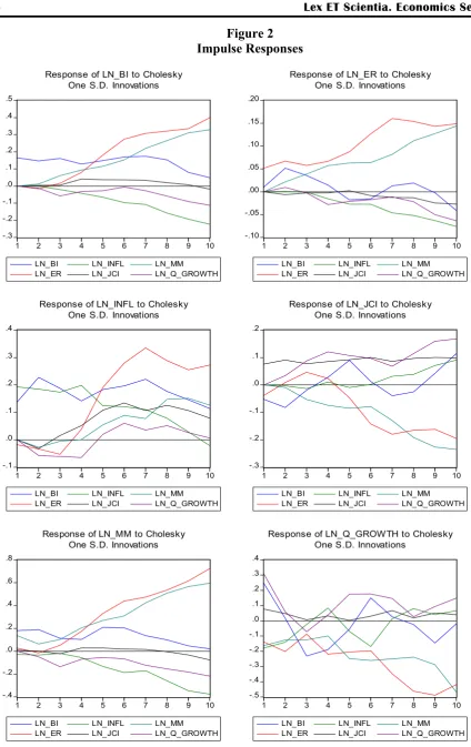
The result confirms that monetary policy in terms BI rate as well as the money market rate are significantly affecting the JCI through the financial system transmission mechanisms. In terms of inflation targeting regime, the central bank plays a role of controlling the inflation target, since it has a significant impact as well to the stock market.

(15)

254

Figure 2 Impulse Responses -.3 -.2 -.1 .0 .1 .2 .3 .4 .5

1 2 3 4 5 6 7 8 9 10

LN_BI LN_ER LN_INFL LN_JCI LN_MM LN_Q_GROWTH

Response of LN_BI to Cholesky One S.D. Innovations

-.10 -.05 .00 .05 .10 .15 .20

1 2 3 4 5 6 7 8 9 10

LN_BI LN_ER LN_INFL LN_JCI LN_MM LN_Q_GROWTH

Response of LN_ER to Cholesky One S.D. Innovations

-.1 .0 .1 .2 .3 .4

1 2 3 4 5 6 7 8 9 10

Response of LN_INFL to Cholesky One S.D. Innovations

-.3 -.2 -.1 .0 .1 .2

1 2 3 4 5 6 7 8 9 10

Response of LN_JCI to Cholesky One S.D. Innovations

-.4 -.2 .0 .2 .4 .6 .8

1 2 3 4 5 6 7 8 9 10

Response of LN_MM to Cholesky One S.D. Innovations

-.5 -.4 -.3 -.2 -.1 .0 .1 .2 .3 .4

1 2 3 4 5 6 7 8 9 10

LN_BI LN_ER LN_INFL LN_JCI LN_MM LN_Q_GROWTH

(16)

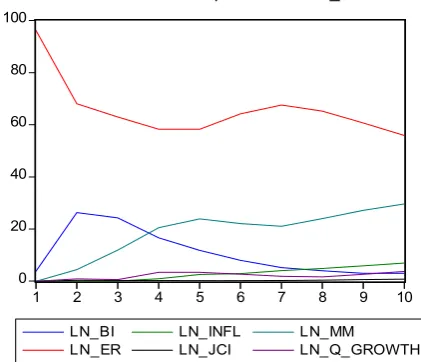
Figure 3 Variance Decomposition 0 20 40 60 80 100

1 2 3 4 5 6 7 8 9 10

Variance Decomposition of LN_BI

0 20 40 60 80 100

1 2 3 4 5 6 7 8 9 10

Variance Decomposition of LN_ER

0 10 20 30 40 50 60 70

1 2 3 4 5 6 7 8 9 10

Variance Decomposition of LN_INFL

0 10 20 30 40 50 60

1 2 3 4 5 6 7 8 9 10

Variance Decomposition of LN_JCI

0 10 20 30 40 50 60 70 80

1 2 3 4 5 6 7 8 9 10

Variance Decomposition of LN_MM

0 10 20 30 40 50

1 2 3 4 5 6 7 8 9 10

(17)

256

Increasingly, from the variance decomposition results (Figure 3) and Table 5 (Appendix), we can investigates that BI rate has most significant influence to the stock market in particular. BI rate has 60% to almost 100% impact on affecting the stock market as well as the other macroeconomic indicators. The exchange rate has 50% to 80 % influence to the stock market performance. The remains are the inflation rate, which has 40% to 70% impact to the stock market. Based on these results, we can determine that the monetary policy has significant effect on the stock market particularly, as well as the macroeconomic stability. In conclusion, the monetary policy is significantly effective to achieve its goals that are the price stability as well as the financial system stability through the stability performance of stock market.

Conclusions and recommendations

Based on the research findings, we conclude that under the inflation-targeting regime, Bank Indonesia significantly has high influence to the macroeconomic stability. Through the monetary policy transmission mechanisms, Bank Indonesia effectively utilizes all the monetary instruments in order to achieve their objectives that are price stability and economic growth. The stance of monetary policy also has a significant impact to the financial system stability. This paper found that the Indonesian stock market are significantly affecting by the monetary policy stance through its instruments such as the Bank Indonesia rate as the single instrument in terms of inflation-targeting framework as well as the money market rate.

(18)

APPENDIX

Table 1

Co-integration Summary

Series: LN_BI LN_ER LN_INFL LN_JCI LN_MM LN_Q_GROWTH Lags interval: 1 to 4

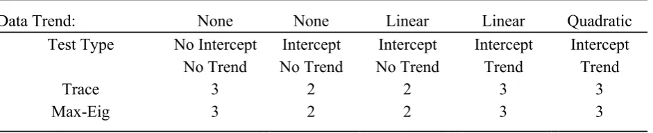
Selected (0.05 level*) Number of Cointegrating Relations by Model

Data Trend: None None Linear Linear Quadratic

Test Type No Intercept Intercept Intercept Intercept Intercept

No Trend No Trend No Trend Trend Trend

Trace 3 2 2 3 3

Max-Eig 3 2 2 3 3

*Critical values based on MacKinnon-Haug-Michelis (1999)

Information Criteria by Rank and Model

Data Trend: None None Linear Linear Quadratic

Rank or No Intercept Intercept Intercept Intercept Intercept

No. of CEs No Trend No Trend No Trend Trend Trend

Log Likelihood by Rank (rows) and Model (columns)

0 242.3670 242.3670 251.0767 251.0767 252.5785

1 275.5736 278.6556 287.3106 292.1720 292.9193

2 300.8015 304.2956 311.4135 316.8723 317.6191

3 314.3332 318.1024 323.1296 336.3877 337.1010

4 320.2289 325.7383 329.2583 347.6872 348.3918

5 321.0073 329.5027 329.7961 353.6467 353.7617

6 321.0090 329.8138 329.8138 354.1598 354.1598

Akaike Information Criteria by Rank (rows) and Model (columns)

0 -4.098624 -4.098624 -4.211529 -4.211529 -4.024102

1 -4.982232 -5.068983 -5.221276 -5.382167 -5.204969

2 -5.533397 -5.595649 -5.725561 -5.869677 -5.734131

3 -5.597218 -5.629265 -5.713734 -6.141155* -6.045875

4 -5.342870 -5.405761 -5.469094 -6.070299 -6.016326

5 -4.875303 -5.020945 -4.991504 -5.776945 -5.740069

6 -4.375375 -4.492240 -4.492240 -5.256657 -5.256657

Schwarz Criteria by Rank (rows) and Model (columns)

(19)

258

1 1.099171 1.051403 1.094028 0.972120* 1.344234

2 1.015806 1.031521 1.057543 0.991393 1.282873

3 1.419786 1.504689 1.537170 1.226698 1.438929

4 2.141934 2.234977 2.249610 1.804338 1.936278

5 3.077302 3.126576 3.195000 2.604476 2.680335

6 4.045029 4.162065 4.162065 3.631548 3.631548

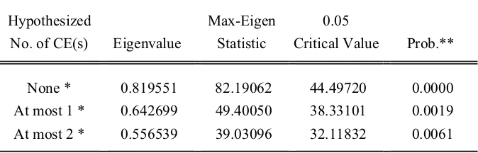
Table 2 Co-integration Test

Trend assumption: Linear deterministic trend (restricted) Series: LN_BI LN_ER LN_INFL LN_JCI LN_MM LN_Q_GROWTH

Lags interval (in first differences): 1 to 4

Unrestricted Cointegration Rank Test (Trace)

Hypothesized Trace 0.05

No. of CE(s) Eigenvalue Statistic Critical Value Prob.**

None * 0.819551 206.1661 117.7082 0.0000

At most 1 * 0.642699 123.9755 88.80380 0.0000

At most 2 * 0.556539 74.57501 63.87610 0.0049

Trace test indicates 3 cointegrating eqn(s) at the 0.05 level * denotes rejection of the hypothesis at the 0.05 level **MacKinnon-Haug-Michelis (1999) p-values

Unrestricted Cointegration Rank Test (Maximum Eigenvalue)

Hypothesized Max-Eigen 0.05

No. of CE(s) Eigenvalue Statistic Critical Value Prob.**

None * 0.819551 82.19062 44.49720 0.0000

At most 1 * 0.642699 49.40050 38.33101 0.0019

At most 2 * 0.556539 39.03096 32.11832 0.0061

Max-eigenvalue test indicates 3 cointegrating eqn(s) at the 0.05 level * denotes rejection of the hypothesis at the 0.05 level

(20)

Unrestricted Cointegrating Coefficients (normalized by b'*S11*b=I):

LN_BI LN_ER LN_INFL LN_JCI LN_MM

LN_Q_GRO

WTH @TREND(2)

10.35325 -9.049707 3.149989 -9.093080 -8.622210 4.829329 0.440746

-22.66537 5.961232 10.05386 3.726592 12.55172 -0.194099 -0.307688

45.52114 -20.84330 -3.821325 -9.786950 -33.35832 -9.164140 0.932197

13.70967 6.218039 -2.876248 2.305123 -12.74163 -2.540873 -0.249530

-4.158835 -3.010891 -4.367122 -2.363666 -0.087369 -2.359213 0.139923

21.56337 -1.997966 -1.211270 0.187089 -17.28400 3.087290 -0.047369

Unrestricted Adjustment Coefficients (alpha):

D(LN_BI) -0.034588 0.004683 -0.031182 0.003658 0.045395 0.002209

D(LN_ER) 0.013699 -0.013940 0.005190 -0.012637 0.008347 1.88E-05

D(LN_INFL) -0.053215 -0.075391 -0.046212 0.049580 0.033444 -0.002540

D(LN_JCI) 0.052760 0.017789 0.011061 0.026492 -0.013210 0.002262

D(LN_MM) -0.092324 -0.016737 -0.011116 -0.011810 0.046285 0.014693

D(LN_Q_GRO

WTH) -0.178801 0.145686 0.092336 0.046959 0.092830 -0.010421

1 Cointegrating Equation(s):

Log

likelihood 292.1720

Normalized cointegrating coefficients (standard error in parentheses)

LN_BI LN_ER LN_INFL LN_JCI LN_MM

LN_Q_GRO

WTH @TREND(2)

1.000000 -0.874093 0.304251 -0.878283 -0.832802 0.466455 0.042571

(0.14779) (0.10058) (0.10143) (0.06077) (0.09594) (0.00710)

Adjustment coefficients (standard error in parentheses)

D(LN_BI) -0.358098

(0.23858)

D(LN_ER) 0.141827

(0.07434)

D(LN_INFL) -0.550943

(0.35070)

D(LN_JCI) 0.546236

(0.14355)

D(LN_MM) -0.955851

(21)

260

D(LN_Q_GRO

WTH) -1.851169

(0.71723)

Log

likelihood 316.8723

LN_Q_GRO

WTH @TREND(2)

1.000000 0.000000 -0.765444 0.142830 -0.433694 -0.188513 0.001096

(0.11016) (0.05293) (0.06751) (0.10631) (0.00156)

0.000000 1.000000 -1.223777 1.168197 0.456597 -0.749312 -0.047450

(0.19819) (0.09523) (0.12146) (0.19127) (0.00281)

D(LN_BI) -0.464237 0.340926

(0.57367) (0.24949)

D(LN_ER) 0.457791 -0.207072

(0.16288) (0.07083)

D(LN_INFL) 1.157822 0.032152

(0.74297) (0.32311)

D(LN_JCI) 0.143041 -0.371417

(0.33233) (0.14453)

D(LN_MM) -0.576502 0.735730

(0.79822) (0.34714)

D(LN_Q_GRO

WTH) -5.153206 2.486565

(1.54298) (0.67103)

Log

likelihood 336.3877

LN_Q_GRO

WTH @TREND(2)

1.000000 0.000000 0.000000 1.261547 -1.002617 -2.437087 -0.013710

(0.19710) (0.24524) (0.38641) (0.00553)

0.000000 1.000000 0.000000 2.956778 -0.452985 -4.344287 -0.071121

(0.35327) (0.43957) (0.69258) (0.00992)

(22)

D(LN_BI) -1.883659 0.990854 0.057284

(1.14385) (0.51781) (0.24703)

D(LN_ER) 0.694057 -0.315254 -0.116837

(0.33431) (0.15134) (0.07220)

D(LN_INFL) -0.945793 0.995360 -0.749006

(1.46041) (0.66111) (0.31539)

D(LN_JCI) 0.646547 -0.601963 0.302774

(0.68121) (0.30837) (0.14712)

D(LN_MM) -1.082534 0.967433 -0.416610

(1.65784) (0.75048) (0.35803)

D(LN_Q_GRO

WTH) -0.949979 0.561984 0.548646

(3.04674) (1.37921) (0.65798)

Log

likelihood 347.6872

LN_Q_GRO

WTH @TREND(2)

1.000000 0.000000 0.000000 0.000000 -0.929843 -0.299282 0.000346

(0.07690) (0.10646) (0.00146)

0.000000 1.000000 0.000000 0.000000 -0.282421 0.666241 -0.038177

(0.18641) (0.25805) (0.00354)

0.000000 0.000000 1.000000 0.000000 -0.658949 -0.460918 -0.003059

(0.15275) (0.21145) (0.00290)

0.000000 0.000000 0.000000 1.000000 -0.057686 -1.694590 -0.011142

(0.18329) (0.25372) (0.00348)

D(LN_BI) -1.833505 1.013602 0.046762 0.645568

(1.18236) (0.53530) (0.25488) (0.30970)

D(LN_ER) 0.520804 -0.393833 -0.080489 -0.256442

(0.31409) (0.14220) (0.06771) (0.08227)

D(LN_INFL) -0.266070 1.303649 -0.891609 0.769493

(1.39991) (0.63380) (0.30177) (0.36669)

D(LN_JCI) 1.009740 -0.437237 0.226578 -0.460644

(23)

262

D(LN_MM) -1.244442 0.894000 -0.382643 0.858708

(1.70938) (0.77391) (0.36848) (0.44775)

D(LN_Q_GRO

WTH) -0.306186 0.853978 0.413580 1.373326

(3.10511) (1.40581) (0.66936) (0.81334)

Log

likelihood 353.6467

LN_Q_GRO

WTH @TREND(2)

1.000000 0.000000 0.000000 0.000000 0.000000 0.606467 0.001925

(0.39345) (0.00545)

0.000000 1.000000 0.000000 0.000000 0.000000 0.941344 -0.037697

(0.24672) (0.00342)

0.000000 0.000000 1.000000 0.000000 0.000000 0.180956 -0.001940

(0.27872) (0.00386)

0.000000 0.000000 0.000000 1.000000 0.000000 -1.638399 -0.011044

(0.24023) (0.00333)

0.000000 0.000000 0.000000 0.000000 1.000000 0.974088 0.001698

(0.46098) (0.00638)

D(LN_BI) -2.022295 0.876922 -0.151483 0.538269 1.346590

(1.06531) (0.48454) (0.24472) (0.28211) (0.76818)

D(LN_ER) 0.486089 -0.418966 -0.116942 -0.276172 -0.305937

(0.30011) (0.13650) (0.06894) (0.07947) (0.21640)

D(LN_INFL) -0.405158 1.202953 -1.037663 0.690443 0.419439

(1.35061) (0.61431) (0.31026) (0.35767) (0.97391)

D(LN_JCI) 1.064679 -0.397462 0.284269 -0.429419 -0.936991

(0.61965) (0.28184) (0.14235) (0.16409) (0.44682)

D(LN_MM) -1.436935 0.754639 -0.584776 0.749305 1.103214

(1.63012) (0.74144) (0.37447) (0.43169) (1.17545)

D(LN_Q_GRO

WTH) -0.692251 0.574476 0.008178 1.153906 -0.316336

(24)

Table 3

Vector Error Correction Estimates

Standard errors in ( ) & t-statistics in [ ]

Cointegrating Eq: CointEq1

LN_BI(-1) 1.000000

LN_ER(-1) -0.058036

(0.03421)

[-1.69654]

LN_INFL(-1) -0.609794

(0.11748)

[-5.19058]

LN_JCI(-1) 0.400955

(0.04936)

[ 8.12346]

LN_MM(-1) -0.550995

(0.07049)

[-7.81609]

LN_Q_GROWTH(-1) -0.759274

(0.11077)

[-6.85466]

C -0.899675

Error Correction: D(LN_BI) D(LN_ER) D(LN_INFL) D(LN_JCI) D(LN_MM)

D(LN_Q_GR OWTH)

CointEq1 0.203848 -0.071771 0.445518 -0.490872 0.846696 1.669149

(0.23643) (0.07548) (0.34197) (0.14323) (0.32896) (0.70039)

[ 0.86219] [-0.95085] [ 1.30278] [-3.42707] [ 2.57387] [ 2.38316]

D(LN_BI(-1)) -0.217087 -0.045523 1.062270 -0.058680 0.558853 -0.213556

(0.44053) (0.14064) (0.63718) (0.26688) (0.61293) (1.30501)

(25)

264

D(LN_BI(-2)) 0.169527 -0.446875 0.509030 0.275451 0.943802 0.889719

(0.58926) (0.18812) (0.85231) (0.35699) (0.81987) (1.74561)

[ 0.28769] [-2.37543] [ 0.59723] [ 0.77160] [ 1.15116] [ 0.50969]

D(LN_BI(-3)) -0.629868 -0.184949 -0.141119 0.551764 -0.676257 -0.117267

(0.70025) (0.22356) (1.01285) (0.42423) (0.97430) (2.07441)

[-0.89948] [-0.82730] [-0.13933] [ 1.30064] [-0.69409] [-0.05653]

D(LN_BI(-4)) -0.428723 -0.111132 -0.318009 0.901665 -0.289989 0.217971

(0.66943) (0.21372) (0.96827) (0.40555) (0.93142) (1.98310)

[-0.64043] [-0.51999] [-0.32843] [ 2.22330] [-0.31134] [ 0.10991]

D(LN_ER(-1)) -0.377615 0.193274 -0.782097 1.229093 -0.815656 -2.751251

(0.77335) (0.24689) (1.11858) (0.46851) (1.07600) (2.29094)

[-0.48829] [ 0.78282] [-0.69919] [ 2.62342] [-0.75804] [-1.20093]

D(LN_ER(-2)) 0.046336 0.109086 -0.166916 0.909954 -0.196198 -1.505673

(0.77678) (0.24799) (1.12354) (0.47059) (1.08078) (2.30111)

[ 0.05965] [ 0.43988] [-0.14856] [ 1.93365] [-0.18153] [-0.65432]

D(LN_ER(-3)) 0.908273 0.020862 1.127799 0.616039 1.184458 -5.287009

(0.63452) (0.20257) (0.91778) (0.38441) (0.88285) (1.87970)

[ 1.43142] [ 0.10298] [ 1.22883] [ 1.60257] [ 1.34163] [-2.81269]

D(LN_ER(-4)) 0.716682 0.036895 0.544772 0.376378 1.114965 -1.988526

(0.85369) (0.27254) (1.23478) (0.51718) (1.18779) (2.52894)

[ 0.83951] [ 0.13537] [ 0.44119] [ 0.72775] [ 0.93869] [-0.78631]

D(LN_INFL(-1)) 0.089072 0.017535 -0.005523 -0.206134 0.235876 0.369709

(0.17601) (0.05619) (0.25458) (0.10663) (0.24489) (0.52141)

[ 0.50606] [ 0.31205] [-0.02169] [-1.93317] [ 0.96318] [ 0.70906]

D(LN_INFL(-2)) -0.096401 0.010390 0.028715 -0.193093 0.031686 0.435568

(0.16459) (0.05255) (0.23806) (0.09971) (0.22900) (0.48758)

[-0.58570] [ 0.19773] [ 0.12062] [-1.93651] [ 0.13837] [ 0.89333]

D(LN_INFL(-3)) 0.021071 -0.089107 0.372959 -0.082716 0.233447 0.982513

(0.16684) (0.05326) (0.24131) (0.10107) (0.23213) (0.49423)

(26)

D(LN_INFL(-4)) 0.019095 -0.077601 0.108241 -0.293269 0.112970 0.383801

(0.13474) (0.04302) (0.19489) (0.08163) (0.18747) (0.39916)

[ 0.14171] [-1.80395] [ 0.55539] [-3.59268] [ 0.60259] [ 0.96153]

D(LN_JCI(-1)) 0.003921 -0.109297 -0.357742 0.270189 -0.218059 -0.162965

(0.27341) (0.08729) (0.39546) (0.16564) (0.38041) (0.80994)

[ 0.01434] [-1.25216] [-0.90462] [ 1.63122] [-0.57322] [-0.20121]

D(LN_JCI(-2)) 0.016509 0.130165 0.306474 0.025535 -0.475988 -0.889240

(0.28488) (0.09095) (0.41205) (0.17259) (0.39637) (0.84392)

[ 0.05795] [ 1.43118] [ 0.74377] [ 0.14796] [-1.20086] [-1.05370]

D(LN_JCI(-3)) 0.331261 0.043106 0.185364 0.236534 0.154038 0.036980

(0.29202) (0.09323) (0.42238) (0.17691) (0.40630) (0.86507)

[ 1.13438] [ 0.46237] [ 0.43886] [ 1.33702] [ 0.37912] [ 0.04275]

D(LN_JCI(-4)) 0.091177 0.023480 0.510628 0.201375 -0.229698 -1.330182

(0.30528) (0.09746) (0.44156) (0.18494) (0.42475) (0.90435)

[ 0.29867] [ 0.24092] [ 1.15641] [ 1.08883] [-0.54078] [-1.47086]

D(LN_MM(-1)) 0.154560 0.156012 -0.178061 -0.206450 -0.252737 0.224512

(0.21429) (0.06841) (0.30995) (0.12982) (0.29815) (0.63480)

[ 0.72127] [ 2.28048] [-0.57449] [-1.59029] [-0.84768] [ 0.35367]

D(LN_MM(-2)) 0.350604 0.203732 -0.048246 -0.450216 -0.225502 -0.450342

(0.27117) (0.08657) (0.39222) (0.16428) (0.37729) (0.80330)

[ 1.29294] [ 2.35334] [-0.12301] [-2.74056] [-0.59769] [-0.56062]

D(LN_MM(-3)) 0.411640 0.215642 -0.491806 -0.339943 0.152559 -0.634931

(0.30370) (0.09696) (0.43927) (0.18399) (0.42255) (0.89966)

[ 1.35543] [ 2.22411] [-1.11960] [-1.84766] [ 0.36104] [-0.70574]

D(LN_MM(-4)) 0.115518 0.156656 -0.045306 -0.257249 -0.044214 -0.857652

(0.27487) (0.08775) (0.39757) (0.16652) (0.38244) (0.81425)

[ 0.42027] [ 1.78521] [-0.11396] [-1.54486] [-0.11561] [-1.05330]

D(LN_Q_GROWTH

(-1)) 0.114801 -0.023565 0.151721 -0.262948 0.483506 0.463191

(0.15865) (0.05065) (0.22947) (0.09611) (0.22074) (0.46998)

(27)

266

D(LN_Q_GROWTH

(-2)) -0.021928 -0.022376 0.163168 -0.150686 0.135826 0.051249

(0.11168) (0.03565) (0.16153) (0.06766) (0.15538) (0.33083)

[-0.19635] [-0.62759] [ 1.01013] [-2.22723] [ 0.87414] [ 0.15491]

D(LN_Q_GROWTH

(-3)) 0.058310 -0.013297 0.103199 -0.091926 0.219655 -0.039201

(0.08697) (0.02777) (0.12580) (0.05269) (0.12101) (0.25765)

[ 0.67043] [-0.47888] [ 0.82035] [-1.74464] [ 1.81515] [-0.15215]

D(LN_Q_GROWTH

(-4)) 0.022898 0.002262 0.131100 -0.012603 0.034756 0.013126

(0.06542) (0.02089) (0.09462) (0.03963) (0.09102) (0.19380)

[ 0.35002] [ 0.10832] [ 1.38550] [-0.31801] [ 0.38185] [ 0.06773]

C -0.039791 -0.003547 -0.049745 0.004253 0.048435 0.166002

(0.04280) (0.01366) (0.06191) (0.02593) (0.05955) (0.12679)

[-0.92969] [-0.25958] [-0.80355] [ 0.16404] [ 0.81333] [ 1.30927]

R-squared 0.436263 0.761059 0.610966 0.760291 0.594376 0.703522

Adj. R-squared -0.204348 0.489534 0.168882 0.487895 0.133439 0.366615

Sum sq. resids 0.597986 0.060948 1.251045 0.219470 1.157625 5.247696

S.E. equation 0.164867 0.052634 0.238465 0.099880 0.229389 0.488397

F-statistic 0.681011 2.802911 1.382013 2.791124 1.289496 2.088179

Log likelihood 37.14028 91.94522 19.42427 61.19668 21.28689 -14.98716

Akaike AIC -0.464178 -2.747717 0.273989 -1.466528 0.196380 1.707799

Schwarz SC 0.549389 -1.734150 1.287556 -0.452961 1.209947 2.721366

Mean dependent -0.001585 0.010661 -0.025929 0.029948 0.020428 -0.006505

S.D. dependent 0.150231 0.073669 0.261574 0.139572 0.246418 0.613676

Determinant resid covariance (dof

adj.) 2.75E-11

Determinant resid covariance 2.55E-13

Log likelihood 287.3106

Akaike information criterion -5.221276

(28)

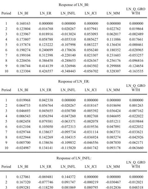
Table 4 Impulse Responses

Response of LN_BI:

Period LN_BI LN_ER LN_INFL LN_JCI LN_MM

LN_Q_GRO WTH

1 0.160163 0.000000 0.000000 0.000000 0.000000 0.000000 2 0.123804 -0.016768 0.020267 0.037941 0.022762 0.019864 3 0.123967 0.018916 -0.013024 0.053093 0.062017 -0.002489 4 0.173807 0.058788 -0.055310 0.085627 0.111886 0.017661 5 0.157874 0.123222 -0.107998 0.083227 0.136434 -0.000461 6 0.190274 0.240699 -0.170636 0.056240 0.180352 -0.028965 7 0.199104 0.312398 -0.220140 0.023307 0.231603 -0.053257 8 0.220436 0.386458 -0.288653 -0.026367 0.256176 -0.096816 9 0.186744 0.414139 -0.326946 -0.043502 0.299888 -0.124654 10 0.123304 0.426557 -0.348443 -0.056702 0.328307 -0.163535

Response of LN_ER:

LN_Q_GRO WTH

1 0.019968 0.042338 0.000000 0.000000 0.000000 0.000000 2 0.064733 0.056764 -0.020267 -0.018167 0.018694 0.001263 3 0.046693 0.045655 -0.030700 -0.005392 0.036424 -0.007162 4 0.006543 0.056394 -0.047260 0.002768 0.046695 -0.022022 5 0.002458 0.079381 -0.063371 -0.002078 0.051211 -0.019844 6 0.012104 0.105050 -0.072313 -0.019536 0.047091 -0.022032 7 0.029744 0.138637 -0.095734 -0.031114 0.063731 -0.033621 8 0.022944 0.142269 -0.104315 -0.036924 0.085274 -0.042926 9 0.005700 0.138636 -0.109832 -0.046556 0.087030 -0.062171

10 -0.024987 0.134141 -0.115820 -0.041742 0.093178 -0.063660

Response of LN_INFL:

LN_Q_GRO WTH

(29)

268

4 0.146653 -0.078772 0.071352 0.122831 0.001112 0.053046 5 0.186895 0.008518 -0.052775 0.164248 0.085802 0.088147 6 0.133853 0.127259 -0.099598 0.132291 0.114310 0.059437 7 0.236380 0.298459 -0.144178 0.015543 0.088525 -0.018553 8 0.213304 0.317802 -0.177028 -0.040336 0.142662 -0.022684 9 0.220682 0.318442 -0.205903 -0.108085 0.138269 -0.083415 10 0.174427 0.244138 -0.193878 -0.090381 0.150786 -0.105948

Response of LN_JCI:

LN_Q_GRO WTH

1 -0.042905 -0.054819 0.002166 0.065172 0.000000 0.000000 2 -0.045060 -0.019375 0.004421 0.053210 -0.012505 0.009509 3 0.048759 0.019091 0.000115 0.002633 -0.054515 0.022840 4 0.064905 -0.004182 0.046393 -0.005143 -0.077056 0.041434 5 0.122103 -0.032890 0.054320 -0.016034 -0.105251 0.037571 6 0.082589 -0.125740 0.108977 0.010299 -0.101354 0.059660 7 0.007729 -0.208414 0.168610 0.028578 -0.157086 0.052693 8 0.015286 -0.246870 0.200378 0.057003 -0.204499 0.092296 9 0.045871 -0.283844 0.248743 0.072750 -0.244156 0.144364 10 0.127514 -0.287951 0.273483 0.072979 -0.269999 0.155745

Response of LN_MM:

LN_Q_GRO WTH

(30)

Response of LN_Q_GROWTH:

LN_Q_GRO WTH

1 0.269433 -0.090345 -0.045216 -0.015000 -0.130273 0.286350

2 0.029384 -0.121644 0.089419 0.068289 -0.098346 0.049432 3 -0.220397 -0.024190 0.174669 0.047969 -0.090307 -0.080380 4 -0.207018 -0.153659 0.135761 -0.050585 -0.088495 -0.030960 5 0.091220 -0.120786 0.069306 -0.088434 -0.221259 0.108420 6 0.146313 -0.184542 0.121115 0.042328 -0.205293 0.118089 7 -0.000431 -0.310345 0.300650 0.104861 -0.188320 0.108897 8 -0.003893 -0.361005 0.281343 0.059687 -0.219787 0.093899 9 -0.034961 -0.342972 0.278592 0.094196 -0.254940 0.185338 10 0.134413 -0.301514 0.328174 0.064006 -0.385533 0.173311

Cholesky Ordering: LN_BI LN_ER LN_INFL LN_JCI LN_MM LN_Q_GROWTH

Table 5

Variance Decomposition

Variance Decomposition of LN_BI:

Pe-riod S.E. LN_BI LN_ER LN_INFL LN_JCI LN_MM

LN_Q_GR OWTH

1 0.160163 100.0000 0.000000 0.000000 0.000000 0.000000 0.000000 2 0.209819 93.08524 0.638696 0.933036 3.269874 1.176876 0.896274 3 0.258051 84.61828 0.959612 0.871563 6.394957 6.553740 0.601846 4 0.351393 70.09944 3.316418 2.947535 9.386713 13.67270 0.577191 5 0.448096 55.52116 9.601448 7.621460 9.222182 17.67869 0.355053 6 0.600479 40.95820 21.41429 12.31915 6.012643 18.86534 0.430384 7 0.776718 31.05094 28.97558 15.39579 3.683681 20.16665 0.727367 8 0.979923 24.56862 33.75758 18.34964 2.386730 19.50431 1.433122 9 1.175113 19.61003 35.89479 20.50097 1.796736 20.07564 2.121821 10 1.355434 15.56698 36.88321 22.01764 1.525476 20.95620 3.050498

Variance Decomposition of LN_ER:

LN_Q_GR OWTH

(31)

270

2 0.103419 42.90589 46.88533 3.840476 3.085861 3.267526 0.014909 3 0.131566 39.10677 41.01186 7.817698 2.074679 9.683438 0.305553 4 0.159497 26.77768 40.40708 14.09917 1.441780 15.16002 2.114280 5 0.196935 17.58000 42.75206 19.60280 0.956850 16.70607 2.402218 6 0.241411 11.95046 47.38607 22.01780 1.291642 14.92253 2.431495 7 0.306120 8.376253 49.98065 23.47348 1.836358 13.61479 2.718465 8 0.368558 6.166097 49.38097 24.20466 2.270571 14.74580 3.231909 9 0.425156 4.651653 47.74166 24.86284 2.905388 15.27142 4.567040 10 0.476726 3.974416 45.88894 25.67717 3.077489 15.96641 5.415576

Variance Decomposition of LN_INFL:

LN_Q_GR OWTH

1 0.204488 38.60885 11.54519 49.84596 0.000000 0.000000 0.000000 2 0.292140 51.71938 12.73881 34.28482 5.61E-05 1.087617 0.169316 3 0.351603 42.74359 20.10138 28.98512 5.280445 0.884133 2.005333 4 0.417529 42.64820 17.81404 23.47484 12.39907 0.627684 3.036164 5 0.504210 42.98454 12.24412 17.19292 19.11392 3.326218 5.138283 6 0.576506 38.27038 14.23840 16.13581 19.88626 6.475836 4.993312 7 0.711704 36.14265 26.92882 14.69159 13.09625 5.796333 3.344363 8 0.840745 32.33623 33.58533 14.96144 9.614794 7.032874 2.469330 9 0.968046 29.58768 36.15400 15.80935 8.498953 7.344934 2.605080 10 1.052074 27.79889 35.99435 16.78083 7.933577 8.272657 3.219696

Variance Decomposition of LN_JCI:

LN_Q_GR OWTH

(32)

Variance Decomposition of LN_MM:

LN_Q_GR OWTH

1 0.232132 59.11700 1.419522 3.849643 0.591756 35.02208 0.000000 2 0.295035 65.50365 0.883323 3.384324 2.570529 27.46894 0.189230 3 0.335971 53.95391 3.645345 3.200138 5.579805 30.26548 3.355324 4 0.472585 37.08797 10.90749 7.813576 6.247631 36.23681 1.706524 5 0.714012 29.31704 18.14948 15.96086 3.876652 31.72620 0.969761 6 0.969466 21.37595 26.00692 19.82640 2.607859 28.85442 1.328452 7 1.232289 14.31371 31.30283 21.07838 1.671340 29.29713 2.336616 8 1.571180 10.63552 35.30700 23.16171 1.182580 26.80129 2.911897 9 1.917741 8.332469 37.15933 24.87003 1.075080 25.20406 3.359022 10 2.243046 6.388744 38.10651 25.45205 1.090085 24.64478 4.317832

Variance Decomposition of LN_Q_GROWTH:

LN_Q_GR OWTH

<