Paper WorldCongress Istanbul Bambang Suprihatin

Delta Method for Deriving the Consistency of Bootstrap Estimator

for Parameter of Autoregressive Model

1_{Bambang Suprihatin,} 2_{Suryo Guritno, and} 3_{Sri Haryatmi} 1_{Mathematics Department, Sriwijaya University, INDONESIA} (Ph.D student of Mathematics Department, Gadjahmada University)

E-mail: suprihatin.b@mail.ugm.ac.id

2,3 _{Mathematics Department, University of Gadjahmada, INDONESIA} E-mail: 2_{suryoguritno@ugm.ac.id}3_{s_kartiko@yahoo.com}

Abstract. Let

{

Xt, t∈T

}

_{be the first order of autoregressive model and let}

X_t

1, Xt2,…, Xtn be the sample that satisfies such model, i.e. the sample follows the relation

X

t

=

θX

t−1

+

ε

t _where

{

εt

}

_{is a zero mean white noise process with}

constant variance σ2 . Let θ^ be the estimator for parameter θ . Brockwell and

Davis (1991) showed that

θ

^

→

p

θ

_and

√

n(θ^−θ)→dN

(

0,σ

2

(

γ^_n(0)

₎

−1

)

_.

Meantime, Central Limit Theorem asserts that the distribution of

√

n

(

X

¯

−

μ

)

converges to Normal distribution with mean 0 and variance σ2 as n→ ∞ _{. In}

bootstrap view, the key of bootstrap terminology says that the population is to the sample as the sample is to the bootstrap samples. Therefore, when we want to investigate the consistency of the bootstrap estimator for sample mean, we

investigate the distribution of

√

n

(

X

¯

¿

− ¯

X

)

contrast to

√

n

(

X

¯

−

μ

)

, where X¯¿ is a bootstrap version of

X

¯

computed from sample bootstrap X¿ . Asymptotic theory of the bootstrap sample mean is useful to study the consistency for many other statistics. Let θ^¿ be the bootstrap estimator for θ^ . In this paper we study the consistency of θ^¿ using delta Method. After all, we construct a measurable map

φ:ℜn→ ℜm _{such that}

√

n

(

_θ^¿

−^θ

)

₌

√

n

(

φ

(

_X¯¿

)

−φ

(

¯_X

)

)

→_dφ'_¯X

(

G

)

conditionally almost surely, by applying the fact that

√

n

(

X

¯

¿

− ¯

X

)

→

_d

G

_{, where}

G is a normal distribution. We also present the Monte Carlo simulations to emphisize the conclusions.

Keywords: Bootstrap, consistency, autoregressive model, delta method, Monte Carlo simulations

Studying of estimation of the unknown parameter θ involves: (1) what estimator

^

θ _{should be used? (2) having choosen to use particular} θ^ _{, is this estimator}

consistent to the population parameter θ _{? (3) how accurate is} θ^ as an

estimator for true parameter θ ? (4) the interesting one is, what is the asymptotic distribution of such estimator? The bootstrap is a general methodology for answering the second and third questions, while the delta method is used to answer the last question. Consistency theory is needed to ensure that the estimator is consistent to the actual parameter as desired.

Consider the parameter θ is the population mean. The consistent estimator

for θ is the sample mean

^

θ= ¯X=1

n

∑

i=1

n

X_i

. The consistency theory is then extended to the consistency of bootstrap estimator for mean. According to the bootstrap terminology, if we want to investigate the consistency of bootstrap

estimator for mean, we investigate the distribution of

√

n

(

X

¯

−

μ

)

and

√

n

(

_X

¯

¿

− ¯

X

)

_{. The consistency of bootstrap under Kolmogorov metric is defined}

as

sup

x

|P_F

(

√

n

(

X¯−μ

)

≤x

)

−P_F n

(√

n

(

¯

X¿

− ¯X

)

≤x

)

|.

(1) Bickel and Freedman (1981) and Singh (1981) showed that (1) converges almost surely to zero as. The consistecy of bootstrap for mean is a worthy tool for studying the consistency and limiting distribution of other statistics. In this paper, we study the

asymptotic distribution of θ^¿ , i.e. bootstrap estimator for parameter of the AR(1) process. Suprihatin, et.al (2013) also studied the advantage of bootstrap for estimating the median, and the results gave a good accuracy.

The consistency of bootstrap estimator for mean is then applied to study the

asymptotic distribution of ^θ¿ , i.e. bootstrap estmate for parameter of the AR(1) process using delta method. We describe the consistency of bootstrap estimates for

consistency of bootstrap estimate for mean under Kolmogorov metric and describe the estimation of autocovariance function. Section 3 deal with asymptotic

distribution of θ^¿ using delta method. Section 4 discuss the results of Monte Carlo simulations involve bootstrap standard errors and density estmation for mean and

^

θ¿

. Section 5, is the last section, briefly describes the conclusions of the paper.

2. Consistency of Bootstrap Estimator For Mean and Estimation of Autocovariance Function

Let

(

X1, X2,…, Xn

)

_{be a random sample of size n from a population with}

common distribution F and let T

(

X1, X2,…, Xn; F

)

_{be the specified random}

variable or statistic of interest, possibly depending upon the unknown distribution F.

Let

F

n _{denote the empirical distribution function of}

(

X1, X2,…, Xn

)

_{, i.e., the}

distribution putting probability 1/n at each of the points

X

1

, X

2

,

…

, X

n _{. The}

bootstrap method is to approximate the distribution of T

(

X1, X2,…, Xn; F

)

_under

F by that of T

(

X1

¿

, X₂¿

,…, X_n¿

; F_n

₎

_under

F

_{n whrere}

₍

X₁¿

, X₂¿

,…, X¿_n

)

_{denotes a}

bootstrapping random sample of size n from

F

n _.

We start with definition of consistency. Let F and G be two distribution

functions on sample space X. Let

ρ

(

F ,G

)

be a metric on the space of distribution

on X. For

X

1

, X

2

,

…

, X

n _{i.i.d from F, and a given functional}

T

₍

X₁, X₂,…, X_n; F

₎

, let

H_n(x)=P_F

₍

T

₍

X₁, X₂,…, X_n; F

₎

≤x

₎

_, H_Boot(x)=P¿

(

T

(

X1¿, X2¿,…, Xn¿; Fn

)

≤x

)

_.

Let functional T is defined as T

(

X1, X2,…, Xn; F

)

=

√

n

(

X¯−μ

)

_where

X

¯

and μ are sample mean and population mean respectively. Bootstrap version of T

is T

(

X1

Mallows metric. The crux result of both papers is that

X

¯

¿

→

_a.s.

¯

X

_{. Suprihatin,}

et.al (2011) emphasized this result by giving nice simulations and agree with their results. Papers of Singh (198) and Bickel and Freedman (1981) have become the foundation for studying other complicated statistics.

Suppose we have the observed values

X

1

, X

2

,

…

, X

n _{from the stationary} AR(1) process. A natural estimators for parameters mean, covariance and correlation

function are μ^n= ¯Xn=

studying the asymptotic properties of the sample autocovariance function γ^n(h) _{, it}

is not a loss of generality to assume that μX = 0. The sample autocovariance

function can be written as

Under some conditions (see, e.g., van der Vaart (2012)), the last three terms in (2) is

of the order

O

p

(

1

/

n

)

_{. Thus, under assumption that} μX = 0, we can write (2) in

simple notation,

^

γ_n(h)=1 n

∑

_t=1

n−h

X_t+hX_t+O_p(1/n) .

The asymptotic behaviour of the sequence

√

n

(

γ

^

n

(

h

)−

γ

X

(

h

)

)

_depends

only on n−1

∑

t=1

n−h

Xt+hXt _{. Note that a change of} n−h _{by n is asymptotically}

negligible, so that, for simplicity of notation, we can equivalently study the average

~_γ

n(h)=

1

n

∑

t=1

n

X_t+hX_t

.

Both γ^n(h) _and ~γn(h) _{are unbiased estimator of} E

(

Xt+hXt

)

=γX(h) _{, under}

the condition that μX=0 _{. Their asymptotic distribution then can be derived by}

applying a central limit theorem to the average

Y

¯

n _{of the variables}

Y

t

=

X

t+h

X

t _.

The asymptotic variance takes the form

∑

g

γ

Y

(

g

)

_{and in general depends on} fourth order moments of the type E

(

Xt+g+hXt+gXt+hXt

)

_{as well as on the}

autocovariance function of the series

X

t _{. Van der Vaart (2012) showed that the}

autocovariance function of the series

Y

t

=

X

t+h

X

t _{can be written as}

V_{h ,h}=κ₄(ε)γ_X(h)2+

∑

g

γ_X(g)2+

∑

g

γ_X(g+h)γ_X(g−h),

(3)

Where

κ₄(ε)=E

(

ε1

4

₎

E

(

ε12

)

2−3,

the fourth cumulant of

ε

t _{. The following theorem}

Theorem 1 If

X

_t

=

μ

+

∑

j=−∞ ∞

ψ

_j

ε

_t−j

holds for an i.i.d. sequence

ε

t _{with mean zero}

and E

(

εt4

)

<∞ _{and numbers}

ψ

j _with

∑

j

|

ψ

j

|<∞

,

_then

√

n

₍

γ

^

_n

(

h

)−

γ

_X

(

h

)

₎

→

_d

N

₍

0,

V

_{h, h}

₎

_.

3. Asymptotic Distribution of Bootstrap Estimate For Parameter of AR(1) Process Using Delta Method

The delta method consists of using a Taylor expansion to approximate a random

vector of the form φ

(

Tn

)

_{by the polynomial} φ(θ)+φ'(θ)

(

Tn−θ

)

+⋯ _in

T

n

−

θ

. This method is useful to deduce the limit law of φ

(

Tn

)

−φ(θ) _{from that of}

T

_n

−

θ

_{, which is guaranteed by the next theorem.}

Theorem 2 Let φ:ℜk→ ℜm be a map defined on a subset of ℜk and

differentiable at θ . Let

T

n _{be random vectors taking their values in the domain}

of

φ

. If rn

(

Tn−θ

)

→dT _{for numbers}

r

n

→∞

_{, then}

r_n

₍

φ

₍

T_n

₎

−φ(θ)

₎

→_dφ_θ'

(T)

. Moreover, the difference between rn

(

φ

(

Tn

)

−φ(θ)

)

and φθ

'

(

r_n

₍

T_n−θ

₎

₎

_{converges to zero in probability.}

Assume that

θ

^

n _{is a statistic, and that}

φ

_{is a given differensiable map. The}

bootstrap estimator for the distribution of

φ

( ^

θ

n

)−

φ

(

θ

)

_is

φ

( ^

θ

n

¿

)−

φ

( ^

θ

_n

)

_{. If the}

bootstrap is consistent for estimating the distribution of

√

n

(

θ^n−θ

)

_{, then it is also}

consistent for estimating the distribution of

√

n

(

φ( ^θn)−φ(θ)

)

_{, as given in the}

Theorem 3 (Delta Method For Bootstrap) Let φ:ℜk→ ℜm be a measurable map

defined and continuously differentiable in a neighborhood of θ . Let

θ

^

n _be

random vectors taking their values in the domain of

φ

that converge almost surely

to θ . If

√

n

(

θ^n−θ

)

→d T _and

√

n

(

θ^n ¿

− ^θ

₎

→_d T _{conditionally almost surely,}

then both

√

n

(

φ

(

θ^n

)

−φ(θ)

)

→dφθ

'

(T) _and

√

n

₍

φ

₍

_θ^

n

¿

)

−φ

₍

_θ^

n

)

)

→d φθ

'

(T)

conditionally almost surely.

Proof. By applying the mean value theorem, the difference

φ

( ^

θ

n

¿

)−

φ

( ^

θ

_n

)

_{can be}

written as φ¯θn

'

(

_θ^

n

¿

−^θ_n

)

_{for a point}

¯

_θ

_n

between

θ

^

n

¿

and

θ

^

n _{, if the latter two}

points are in the ball around θ in which

φ

is continuously differentiable. By the

continuity of the derivative, there exists a constant δ>0 for every

η

>

0

such that ||φθ'

'

−φ_θ'_h

|| _<

_η

_||

_h

_||

_{for every h and every ||θ}'

−θ|| ≤δ _{. If n is}

suffeciently large, δ suffeciently small,

√

n

||^

θ

n

¿

−^

θ

_n

|| ≤

M

_{, and}

||^

θ

_n

−

θ

|| ≤

δ

_{, then}

R

_n

:

=‖

√

n

(

φ

( ^

θ

¿_n

)−

φ

( ^

θ

_n

)

)

−

φ

_θ'

√

n

(

θ

^

_n¿

− ^

θ

_n

)

‖

=|

(

φ¯θn

'

−φ_θ'

₎

_√

n

₍

θ^_n¿_−^θ

n

)

|≤ηM

.

Fix a number ε>0 and a large number M. For η sufficiently small to ensure

that

ηM

<

ε

,

P

₍

R_n>ε| ^P_n

₎

≤P

₍

√

n||^θ_n¿

−^θ_n|| >M or ||^θ_n−θ||>δ| ^P_n

₎

_{. (4)}

Since

θ

^

n

→

a.s.

θ

_{, the right side of (4) converges almost surely to}

P

(

||

T

||≥

M

)

of M. Conclude that the left side of (4) converges to zero almost surely. The theorem follows by an application of Slutsky’s lemma. ■

For the AR(1) process, from Yule-Walker equation we obtain the moment

estimator θ^= ^ρ1 _where ρ^1 _{be the lag 1 sample autocorrelation} demonstrate results of Monte Carlo simulations consist the two of standard errors and give brief comments. In Suprihatin, et.al. (2012) we construct a measurable

function

φ

as follows. Equation (5) can be written as

Brockwell and Davis (1991) have shown that ρ^1 is consistent estimator of

E

₍

X_t−1ε_t

₎

_{= 0. Hence,} 1_n

∑

t=2

n

X_t−1ε_t→_a.s.0

. By applying the Slutsky’s lemma,

the last display is approximated by ~_ρ

x _{. Since}

φ

_{is continous and hence is measurable. Suppose that}

^

ρ

_{is based on a sample from a distribution with finite first four moments of}

ε

_t

.

By central limit theorem and applying Theorem 1 we conclude that

√

n

₍

X

2

−

γ

_X

(

0

)

)

→

_d

N

₍

0,

V

_0,0

₎

_, as follows [see, e.g. Efron dan Tibshirani (1986) and Freedman (1985)]:

^

2. A bootstrap sample

X

1

with replacement from the residuals. Letting X1

¿ 3. Finally, after centering the bootstrap time series

X

1

¿

computed from the sample

X

1

¿

, X

₂¿

,

…

, X

_n¿

.

Analog with the previous discussion, we obtain the bootstrap version for

counterpart of ~ρ1 , that is measurable map

converges to ~ρ1 _{conditionally almost surely.}

By the Glivenko-Cantelli lemma and applying the plug-in principle, we obtain

√

n

₍

X

¿2

_−^

_γ

4. Results of Monte Carlo Simulations

transactions on March and April 2012. Suprihatin, et. al. (2012) has identified that the time series data satisfies the AR(1) procces, such that the data follows the equation

X

_t

=

θX

_t−1

+

ε

_t

, t

=

2, 3,

…

,

50

,

where

ε

t _WN

(

0, σ2

)

_{. The simulation yields the estimator} θ^ ₌ -0.448 with standard error 0.1999. To produce a good approximation, Efron and Tibshirani (1986) and Davison and Hinkley (2006) suggest to use the number of resamples at least B = 50. Bootstrap version of standard errror using bootstrap samples of size B = 25, 50, 100, 1,000 and 2,000 yielding as presented in Table 1.

Table 1 Estimates for Standard Errors of θ^¿ for Various B B

25 50 100 500 1,000 2,000

se_^F

(

_θ^¿

₎

0.2005 0.1981 0.1997 0.1991 0.1972 1.1964

From Table 1 we can see that the values of bootstrap standard errors tend to decrease in term of size of B increase and closed to the value of 0.1999 (actual standard error). These results show that the bootstrap gives a good estimate.

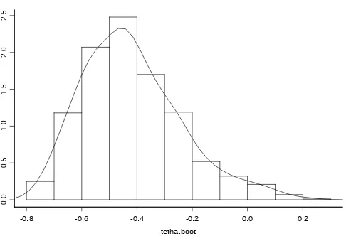
Meantime, the histogram and density estimate of θ^¿ are presented in Figure 1. From Figure 1 we can see that the resulting histogram close related to the normal density. Of course, this result agree to the result of Freedman (1985) and Bose (1988).

-0.8 -0.6 -0.4 -0.2 0.0 0.2

0.

0

0.

5

1.

0

1.

5

2.

0

2.

Figure 1 Histogram and Density Estimate of Bootstrap Estimator θ^¿

5. Conclusions

A number of points arise from the study of Section 2, 3, and 4, amongst which we state as follows.

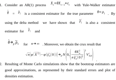
1. Consider an AR(1) process

X

t

=

θX

t−1

+

ε

t _{with Yule-Walker estimator}

^

θ ₌ ρ^_{1 is a consistent estimator for the true parameter} θ=ρ_{1 . By}

using the delta method we have shown that ~ρ1

¿

is also a consistent

estimator for ~ρ1 _and

θ

^

→

p

~

ρ

1 _for n→ ∞ _{. Moreover, we obtain the crux result that}

√

n

(

φ

(

X¿2

₎

_{−φ( ^γ}

n ¿

(0))

)

→_dN

(

0,

(

θXn 2

n^γ_n¿

(0)2

)

2

V_0,0¿

)

_.

2. Resulting of Monte Carlo simulations show that the bootstrap estimators are good approximations, as represented by their standard errors and plot of densities estimation.

REFERENCES

[1] BICKEL, P. J. AND FREEDMAN, D. A. Some asymptotic theory for the bootstrap, Ann. Statist., 9, 1996-1217, 1981.

[2] BOSE, A. Edgeworth correction by bootstrap in autoregressions, Ann. Statist., 16, 1709-1722, 1988.

[3] BROCKWELL, P. J. AND DAVIS, R. A. Time Series: Theory and Methods, Springer, New York, 1991.

[5] EFRON, B. AND TIBSHIRANI, R. Bootstrap methods for standard errors, confidence intervals, and others measures of statistical accuracy, Statistical Science, 1, 54-77, 1986.

[6] FREEDMAN, D. A. On bootstrapping two-stage least-squares estimates in stationary linear models, Ann. Statist., 12, 827-842, 1985.

[7] SINGH, K. On the asymptotic accuracy of Efron’s bootstrap, Ann. Statist., 9, 1187-1195, 1981.

[8] SUPRIHATIN, B., GURITNO, S., AND HARYATMI, S. Consistency of the bootstrap estimator for mean under kolmogorov metric and its implementation on delta method, Proc. of The 6th_{Seams-GMU Conference, 2011.}

[9] VAN DER VAART, A. W. Asymptotic Statistics, Cambridge University Press, Cambridge, 2000.