Normal Moveout Coefficients for Horizontally Layered Triclinic Media

Normal moveout coefficients for horizontally

layered triclinic media

Zvi Koren

1

and Igor Ravve

1

ABSTRACT

Sedimentary layers affected by vertical compaction and strong lateral tectonic stresses are often characterized by low anisotropic symmetry (e.g., tilted orthorhombic [TOR]/monoclinic or even triclinic). Considering all types of pure-mode and converted waves, we derive the normal moveout (NMO) series coefficients of near normal-inci-dence reflected waves in arbitrarily anisotropic horizontally layered media, for a leading error term of order six. The NMO series can be either a function of the invariant hori-zontal slowness (slowness domain) or the surface offset (off-set domain). The NMO series coefficients, referred to also as effective parameters, are associated with the corresponding azimuthally varying NMO velocity functions. We distin-guish between local (single-layer) and global (overburden multilayer) effective parameters, which are related by for-ward and inverse Dix-type transforms. We derive the local effective parameters for an arbitrary anisotropic (triclinic) layer, which is the main contribution of this paper. With some additional geologic constraints, the local effective parameters can then be converted into the interval elastic properties. To demonstrate the applicability of our method, we consider a synthetic layered model in which each layer is characterized with TOR symmetry. The corresponding global effective model loses the symmetries of the individual layers and is characterized by triclinic symmetry.

INTRODUCTION

Triclinic rocks are the most general anisotropic continua, charac-terized by point symmetry only (at each given point, the continuum is symmetric under reflection through the origin of the coordinate frame, located at this point), and its stiffness matrix includes 21

dis-tinct components (e.g.,Slawinski, 2015). Subsurface sedimentary

layers affected by vertical compaction and lateral asymmetric tec-tonic stress typically exhibit considerable azimuthal anisotropy. In many cases, under these conditions, the anisotropic symmetries break down and the layers can only be described by triclinic anisotropy. Overall, symmetries lower than orthorhombic in hori-zontally layered media could be caused by complex fracture sys-tems or stress regimes resulting in considerable azimuthal

anisotropy (e.g.,Grechka and Kachanov, 2006;Lynn and

Michel-ena, 2011;Jones and Davison, 2015). In these cases, transverse isotropy with a tilted axis of symmetry (TTI) is insufficient to ex-plain the azimuthal anisotropy, and, at least, a tilted orthorhombic (TOR) model is needed for these complex geologic structures (Li et al., 2012). The presence of multiple fracture sets may lower the medium symmetry to monoclinic or even triclinic. If multiple fracture sets have their normals confined to the same plane, then that plane is the plane of symmetry, and the medium is monoclinic (Bakulin et al., 2000b); otherwise, it is triclinic (Tsvankin and Grechka, 2011). Note that even in cases in which the individual layers are characterized by different TOR parameters, the global effective model is characterized by general (triclinic) anisotropy, in which the symmetries of the individual layers are completely ruined.

The literature on normal moveout (NMO) approximations in anisotropic layered media is very rich and includes important stud-ies, which have already been extensively implemented in seismic processing and imaging. The forward computation of second-order global NMO velocities (NMO velocity ellipse) in layered ortho-rhombic media as a function of the offset azimuth (source-receiver

azimuth) ψoff has been intensively studied (e.g., Grechka and

Tsvankin, 1998; Bakulin et al., 2000a, 2002). This theory has been extended for depth-varying orientation of the vertical

symmetry planes by Grechka and Tsvankin (1999). Ravve and

Koren (2013, 2015a), Koren et al. (2013), and Koren and Ravve (2014)study the second-order NMO velocity for the same layered orthorhombic model as a function of the slowness

azi-muthψslw.

Manuscript received by the Editor 18 November 2016; revised manuscript received 4 April 2017; published online 27 June 2017.

1_{Paradigm Geophysical, Herzliya, Israel. E-mail: zvi.koren@pdgm.com; igor.ravve@pdgm.com.}

© 2017 Society of Exploration Geophysicists. All rights reserved.

WA119 10.1190/GEO2016-0595.1

For pure-mode waves, Grechka et al. (1997, 1999) derive a general equation for the NMO ellipse in arbitrarily anisotropic, homogeneous media and introduce a 3D generalized Dix-type equa-tion for layered media above the horizontal and dipping reflectors. Grechka and Tsvankin (2002a)further extend the generalized Dix-type procedure to obtain the effective NMO ellipses in laterally heterogeneous, arbitrarily anisotropic media. These results have been used in stacking velocity-driven tomography for interval parameter estimation in transversely isotropic and orthorhombic

media (Grechka et al., 2005). Hao and Stovas (2016)study the

slowness surface approximation for P-waves and acoustic model

in a homogeneous TOR media.Ivanov and Stovas (2016)derive

the second-order NMO velocity formula for a single-layer TOR medium considering pure-mode and converted waves.

Overall, the second-order moveout approximations may provide an acceptable fit to P-wave reflection traveltimes for offset-to-depth

ratio up to one and moderate anisotropy (Grechka and Tsvankin,

1999; Vasconcelos and Grechka, 2007; Tsvankin and Grechka, 2011;Tsvankin, 2012). However, it has been shown that the accu-racy of hyperbolic moveout equations parameterized by second-or-der NMO velocities is not sufficient for analyzing seismic reflection events with longer offsets, (when the offset-to-depth ratio exceeds one), especially in azimuthally anisotropic layered models with low

symmetries and strong anisotropy (e.g.,Koren and Ravve, 2017;

Ravve and Koren, 2017b). In these cases, the use of hyperbolic approximation is questionable and can cause significant errors in the inversion; therefore, higher order terms become essential. Even for pure-mode P-waves and short offsets, in the case of TOR or triclinic layered media, it may be necessary to include nonhyper-bolic terms.

Nonhyperbolic reflection moveout in a layered transversely iso-tropic medium with a horizontal symmetry axis (HTI) has been

stud-ied in the offset-azimuth domain byAl-Dajani and Tsvankin (1998)

and in the slowness-azimuth domain byRavve and Koren (2010)and

Koren et al. (2010).Al-Dajani et al. (1998)andAl-Dajani and Toksoz (2001)derive the offset-azimuth domain fourth-order moveout coef-ficient for a single orthorhombic layer with a horizontal symmetry

plane, which overlies a horizontal reflector.Pech et al. (2003)derive

an exact equation for the quartic moveout coefficient of pure-mode waves in arbitrarily anisotropic, heterogeneous media, and implement their theory for a transversely isotropic layer with a tilted axis of

sym-metry (TTI).Pech and Tsvankin (2004)study the quartic moveout

coefficient for a dipping orthorhombic layer, considering weak anisotropy and assuming that one of the symmetry planes is aligned with the dip plane of the reflector.

Vasconcelos and Tsvankin (2006)demonstrate that the general-ized version of the nonhyperbolic moveout equation proposed by Alkhalifah and Tsvankin (1995) for vertical symmetry axis (VTI) media gives an accurate description of P-wave moveout in layered orthorhombic models with arbitrary orientation of the

ver-tical symmetry planes.Wang and Tsvankin (2009)present a stable

algorithm for interval moveout inversion in layered orthorhombic media based on velocity-independent layer stripping. This method operates with interval traveltimes that can be obtained without knowledge of the velocity model; this is a key advantage of that approach, which leads to enhanced stability. A comprehensive over-view of second- and fourth-order moveout coefficients and move-out-based parameter estimation for practical anisotropic models is

given in the book byTsvankin and Grechka (2011).

Stovas (2015)studies the NMO velocity in multilayer orthorhom-bic media with different azimuths of the orthorhomorthorhom-bic vertical sym-metry planes, and derives approximate expressions for effective anellipticity in the slowness- and offset-azimuth domains, for

P-waves and acoustic model.Sripanich and Fomel (2016)propose

an explicit formula for the fourth-order NMO velocity for horizon-tally layered triclinic media, considering pure-mode waves with symmetric moveout, which was used to estimate the interval param-eters of layered orthorhombic models with depth-varying azimuths

of vertical symmetry planes.Stovas (2017)derives approximations

for three anelliptic parameters for pure-mode and converted waves

in elastic orthorhombic media.Ravve and Koren (2016,2017b) and

Koren and Ravve (2016a, 2017) derive exact fourth-order NMO velocity functions for all types of pure-mode and converted waves in layered orthorhombic media with depth-varying azimuths of the vertical symmetry planes, for the slowness-azimuth and offset-azi-muth domains.

For large offset-to-depth ratios approaching and exceeding two, even the quartic Taylor series for squared traveltime does not suf-fice, and additional information about the asymptotic horizontal velocity is needed. The moveout approximation for this case was

suggested for layered VTI media by Tsvankin and Thomsen

(1994) and, as discussed by Tsvankin and Grechka (2011), it can be extended to azimuthally anisotropic media with low

sym-metries (Ravve and Koren, 2015b). High accuracy of the long-offset

moveout approximation may be achieved by using additional effec-tive parameters related to a ray at a large finite offset, such as in the

generalized moveout approximation by Fomel and Stovas (2010)

and its modifications (Sripanich and Fomel, 2015; Ravve and

Koren, 2017a;Sripanich et al., 2017).

For models without a horizontal symmetry plane, moveouts of converted waves, even in horizontally layered anisotropic media, become asymmetric (the reflection traveltime changes when the source and receiver are swapped), and the moveout series includes odd and even powers of offset. It may not be easy to operate with the additional moveout coefficients and asymmetric traveltime func-tions in velocity analysis. An attractive alternative (PP + PS =

SS method) is suggested byGrechka and Tsvankin (2002b); the

method makes it possible to obtain the moveout of pure SS-waves from PP and PS data.

Koren and Ravve (2016b)derive the coefficients of the moveout series for general anisotropic (triclinic) layered models, and present this work as an extended abstract at the 17th International Workshop on Seismic Anisotropy. The primary objective of this study is to provide a full derivation of the results presented in that abstract. Considering all types of pure-mode and converted waves, we derive the NMO series coefficients of near normal-incidence reflection waves in general anisotropic (triclinic) horizontally layered media, for a leading error term of order six in offset or horizontal slowness. The body of the paper includes two main parts. In the first, we consider events with symmetric moveout when the traveltime is an even function of the offset or horizontal slowness. This case in-cludes pure-mode waves for general anisotropic horizontally lay-ered media and converted waves for horizontally laylay-ered models sharing a common horizontal symmetry plane. We then introduce an additional intuitive set of normalized parameters for symmetric moveout and provide their feasible ranges. We further show that for weak azimuthal anisotropy, the azimuth in the formulas may be considered generic (i.e., the same in the slowness- and

muth domains), and the second- and fourth-order NMO velocity formulas in the offset-azimuth domain reduce to simpler expres-sions in the slowness-azimuth domain. In the second part, we con-sider converted waves in arbitrarily anisotropic media, in which the moveout becomes asymmetric. Thus, in addition to the three sec-ond-order and five fourth-order effective parameters needed for pure-mode waves, 12 new parameters (two first-order, four third-order, and six fifth-order) are required. The six fifth-order param-eters can be ignored in case we restrict the leading error term to order five.

The validity of the derived formulas for pure-mode waves is dem-onstrated using a synthetic layered model composed of strongly anisotropic TOR layers with varying orientation of all three mutu-ally orthogonal symmetry planes, resulting in an effective velocity model with triclinic symmetry. Each layer is characterized by nine

orthorhombic parameters usingTsvankin (1997) notation,

thick-ness, and three additional Euler angles. The validity of the derived formulas for effective parameters is tested by introducing the offset-azimuth domain, second-order NMO velocity, and fourth-order anellipticity parameter into the well-known, azimuthally varying,

nonhyperbolic moveout approximation (e.g., Vasconcelos and

Tsvankin, 2006). We compare the approximate traveltimes with those obtained by exact ray tracing.

BASIC DEFINITIONS Normal incidence ray pair

Normal incidence means that the incidence and reflection phase-velocity directions are normal to the reflection surface. In the case of horizontal reflectors considered in this study, normal incidence means strictly vertical incidence and reflected phase-velocity vec-tors. The group velocities in this case are generally nonvertical (un-less the horizontal reflector coincides with a plane of symmetry). In the case of normal incidence (vertical slowness vectors), the direc-tions of the incidence and reflected tilted ray (group) velocities coincide for pure-mode waves in triclinic media. In this case, the

offset is zero — the source and receiver locations are the same,

although this lateral location does not coincide with the projection of the reflection point onto the surface. For normal-incidence con-verted waves, in which the moveout is asymmetric, the incidence and reflected phase velocities are still vertical (normal to the reflec-tor), and the two ray velocities are tilted, but the

directions of the incidence and reflection ray velocities are different. In this case, the two nor-mal-incidence rays emerging from the subsurface image point arrive at two different surface points, thus producing a nonzero offset of normal inci-dence. In other words, normal incidence means vanishing horizontal slowness. For an asymmet-ric moveout (e.g., converted waves even in a sin-gle triclinic layer), the zero offset does not mean a normal-incidence ray pair. A normal-incidence ray pair leads to a nonzero offset (which is not small unless the anisotropy is weak), and other ray pairs that differ from the normal incidence ray (i.e., with nonzero horizontal slowness of specific magnitude and azimuth) may lead to a zero surface offset.

Interval, local effective, and global effective parameters We distinguish between three different types of parameters: in-terval parameters, local effective parameters, and global effective parameters. The interval parameters are the physical elastic param-eters of the individual layers. Although not essential, in this study, they are assumed to be constant within each layer, with discontinu-ities across the interfaces. For example, for a TOR layer, these are

the velocity of P-waves propagating in the direction ofx3, the

veloc-ity of S-waves propagating in the direction ofx3, and polarized in

the direction of x1 (where x1; x2; x3 are the intersections of the

orthorhombic symmetry planes constituting the axes of the local

frame), seven Tsvankin’s (1997) orthorhombic parameters, three

Euler orientation angles for the planes of symmetry with respect to the global frame, and the layer thickness. For a fully triclinic layer, these may be 21 density-normalized stiffness coefficients and the layer thickness. The local effective parameters are different

— they are the moveout coefficient parameters of a single layer

(referred to also as interval moveout parameters). Applying forward

“Dix-type”summation over the local effective parameters, we

ob-tain the global effective parameters for the entire medium above the reflector. Note that local and global effective parameters for layered

isotropic media (e.g.,Dix, 1955) have been widely used for interval

velocity parameters estimation and seismic imaging.

In the case of symmetric moveout, for each triclinic layer, there are three second-order and five fourth-order local effective param-eters, all of which are independent. The corresponding overburden layered model is also characterized by eight independent parameters (global effective parameters). Moveout series expansion coeffi-cients are azimuthally dependent functions that include the global effective parameters. Each local effective parameter depends on the derivatives of the vertical slowness (slowness surface) of the corre-sponding order with respect to the horizontal-slowness components and on the layer thickness. For each wave type, the derivatives, computed in this work for the normal-incidence ray with vanishing horizontal slowness, depend only on the stiffness coefficients.

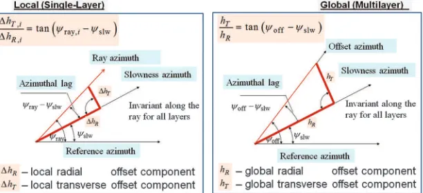
Radial and transverse offset components

It is convenient to split the offset vectorh into the radial

com-ponenthRalong the slowness-azimuthψslwand the transverse

com-ponent hT in the normal direction, ψslwþπ∕2 (as shown in

Figure1, whereh2_¼h2

Rþh2T). A right triangle is shown in red,

Figure 1. Cartoon of the local and global radial (lengthwise) and transverse offset com-ponents, with an azimuthal lag between the offset azimuth and the slowness azimuth.

whose legs arehR andhT. LeghRis in line with the

slowness-azi-muthψslw, and the hypotenusehis in line with the offset-azimuth

ψoff. The acute angle adjacent to leg hR is the azimuthal lag

ψoff−ψslw.

METHOD

We start with the simpler case, assuming a symmetric moveout with only even powers of the offset or horizontal slowness. The moveout is symmetric for pure-mode waves in any media, including the horizontally layered triclinic model treated here. Note that for converted waves, the moveout symmetry holds only for horizontally layered models sharing a horizontal symmetry plane, such as mono-clinic and its particular cases: orthorhombic or transverse isotropy with a VTI or HTI. For the symmetric moveout, the odd-power co-efficients of the NMO series vanish, and the remaining coco-efficients are the zero-offset time and azimuthally varying second-order (three effective parameters) and fourth-order (five effective parameters) NMO velocity functions (for a leading error term of order six). The quartic coefficient can be calculated from the second- and fourth-order NMO velocities. We then extend the theory to cases in which the moveout symmetry no longer holds, i.e., for converted waves in horizontally layered media without a horizontal symmetry plane, such as transverse isotropy with TTI, TOR, tilted monoclinic, and triclinic. In this case, to maintain an error of order six in offset or horizontal slowness, all odd- and even-power coefficients of the NMO series to the fifth order are required. This result in an addi-tional 12 effective parameters: two first-order, four third-order, and six fifth-order. We note that the last six fifth-order parameters can in some cases be optional. By neglecting them, the accuracy of the NMO series will reduce to the fourth order with a leading error term of order five.

Our derivation starts with the so-called local kinematic compo-nents: two offset components and traveltime within a given layer, as series expansions of the short (invariant) horizontal-slowness vec-tor. Its magnitude is small compared with the critical horizontal slowness, in which the latter yields a zero vertical slowness for a given wave type and slowness azimuth. We then invert the series expansion to obtain the traveltime series directly versus the short horizontal-offset vector (small offset-to-depth ratio). The two vec-tors (horizontal slowness and horizontal offset) are then presented in polar frames (with the magnitude and azimuth instead of two Car-tesian components), to obtain azimuthally varying NMO velocities. The latter characterize azimuthally varying moveouts, which are the series expansions in the magnitude of horizontal slowness or hori-zontal offset. We consider the two commonly used azimuthal do-mains: slowness azimuth, in which the moveout is a function of the azimuth and magnitude of the horizontal-slowness vector, and off-set azimuth, in which the moveout is a function of the azimuth and magnitude of the source-receiver offset vector. We note that the same effective parameters are used to approximate the moveouts in the slowness- and offset-azimuth domains, but the explicit ex-pressions of the azimuthally varying NMO velocities are domain dependent. Finally, we provide the two-way relationships between the offset azimuth and slowness azimuth.

The choice of the given azimuth domain depends on the appli-cation and the type of prestack seismic data used. Obviously, when recorded seismic data, such as common shot or common midpoint time gathers, are directly used, offset-azimuth domain NMO veloc-ities are required. However, many applications and workflows,

especially those involved in the velocity analysis for azimuthally anisotropic media, are implemented directly in the migrated domain, using different types of common-image gathers (CIG). The most common CIG types used are those generated by Kirch-hoff-based migration, in which the recorded seismic events are migrated (mapped) down to the subsurface image points and are binned either into offset-azimuth/offset tiles or into slowness-azimuth/horizontal-slowness tiles. The latter are associated with

mi-gration in the local angle domain (e.g.,Koren and Ravve, 2011;

Ravve and Koren, 2011) and have been proven to provide superior image quality, especially for anisotropic velocity-model building and amplitude inversion. General workflows for estimating azimu-thally anisotropic model parameters in the migrated domain, using the concept of effective model parameters, are discussed in a sep-arate section.

SLOWNESS-AZIMUTH ONE-WAY LOCAL KINEMATIC COMPONENTS

Consider a ray emerging from a subsurface point with a given

slowness vector p¼ fp1; p2; p3gand traveling up to the surface

through a set of homogeneous horizontal arbitrarily anisotropic (triclinic) layers. The components of the horizontal slowness

vector ph¼ fp1; p2gare preserved along the entire raypath, and

therefore represent invariant ray parameters. The vertical slowness

p3¼qðphÞ, however, changes from layer to layer. For convenience,

we split the 3D ray-velocity vector into a 2D horizontal ray-velocity

vectorvray;h¼ fvray;1; vray;2gand a scalar vertical ray-velocity

com-ponentvray;3. The ray velocity can be obtained by (Grechka et al.,

1997,1999)

taining the derivatives of the vertical slowness with respect to the horizontal slowness components. Hence, for a general

azimu-thally anisotropic layer with a thickness Δz and with

density-normalized stiffness parametersCij; i; j¼1; : : : ;6, and for a given

horizontal-slowness vectorph, the local kinematic components —

one-way local offset vectorΔhone-way_{and one-way local traveltime}

Δtone−way

Note that the local offset and traveltime,Δhone-way_andΔtone-way_{, can}

also be obtained without the knowledge of the ray-velocity

compo-nents, by using the local intercept timeΔτone-way. Equation set2can

then be written as

For example,Hake (1986),Chapman (2004), andStovas and Fomel

(2012)apply equation3in a scalar form for azimuthally isotropic

layered media. The vertical slownessqðphÞmay be written as a sixth-order polynomial equation using the Christoffel equation

(see AppendixA), where the six roots correspond to three upgoing

and three downgoing wave modes. The vertical slowness values for upgoing and downgoing waves of the same type do not necessarily have opposite signs, but their corresponding vertical components of the ray velocities do. The explicit expressions for the coefficients of

the six-order polynomial equation are given in AppendixB.

Equa-tions1and2are valid for the whole range of horizontal slowness

(whose upper limit corresponds to vanishing vertical slowness for a given wave type). However, our goal is to approximate the local kinematic components (or ray velocity components) by a Taylor series for a small magnitude of horizontal-slowness vector, with

a leading error term of order six. The vertical slownessqðp1; p2Þ

may be expanded into the series in the proximity of the normal incidence:

where the normal-incidence slownessqois related to the local

one-way normal-incidence timeΔtone-wayo , qo¼Δtone-wayo ∕Δz, and qn

are symmetric tensors of then-th derivative of the vertical slowness

with respect to the horizontal slowness components for the normal-incidence ray. The tensor derivatives, together with the symbolic

scalar productqn·pnh, are given by

The number of distinct parameters for each symmetric tensor derivative exceeds its order by one. For example, the second tensor

derivativeq2has three distinct componentsfq;11; q;12; q;22g, and the

symmetric tensor of the fourth derivativesq4has five distinct

com-ponents fq;1111; q;1112; q;1122; q;1222; q;2222g. The near

normal-incidence symmetric tensor derivatives for triclinic media are given

in AppendixC. They depend on the tensor derivatives of the

coef-ficients of the polynomial equation. We emphasize that the

travel-time expression in equation 5 does not contain the linear term

q1·ph. This is because the linear terms in the series expansions

of qðp_hÞ and ph·∇phqðphÞ are equal and cancel each other out

in equation2.

PART 1: PURE-MODE WAVES

In this part, we consider pure-mode waves that have symmetric moveouts.

Slowness-azimuth two-way local kinematic components Considering a two-way path for pure-mode waves, the slowness surface and its derivatives are the same for the incidence and re-flected rays. Further considering that both rays emerge from a sub-surface reflection point, we define

pre_{h ¼}ph; pinh ¼−ph; (7)

where superscripts“in”and “re”are related to the incidence and

reflection rays, accordingly. Thus, the slowness azimuths of the

in-cidence and reflection rays differ byπ. Note that equation7is valid

not only for pure-mode waves but also for converted waves; however, for converted waves, the normal-incidence

vertical-slowness qo and the derivative tensors of the vertical slowness

q1;q2; : : : ;q5are different for the two different wave types (inci-dent and reflected). For pure-mode waves,

Δhre

To obtain the local two-way offsetΔh, we subtract the local incident

and reflected offset vectors (because both rays emerge from the

re-flection point). To obtain the two-way local traveltimeΔt, the local

incident and reflected traveltimes are added. This leads to an odd series for local two-way offsets and an even series for local two-way traveltimes (for pure-mode waves only),

Δh

As we see in equation 8, the fifth-order derivative tensor q5 is required only for converted waves. For two-way pure-mode waves,

q5 is canceled, along with the other odd derivatives q1 and q3

(equation9).

Slowness-azimuth two-way global kinematic components

As mentioned, becausephis constant along the raypath (for all

layers), the two-way global kinematic components can be obtained by a straightforward summation of the local kinematic components of the overburden layers

where indexiis the running number of a layer in the summation.

Next, we introduce two global tensors representing the weighted stacks over the corresponding local tensors, where the weights are the layer thicknesses:

For continuous vertically varying medium properties with pos-sible discontinuities at the interfaces between the layers, the sums can be replaced by integrals. The global offset and traveltime become

wheretois the global two-way normal-incidence time (which is also

the zero-offset time for pure-mode waves). The normal-incidence two-way traveltime, corresponding to a vanishing horizontal slow-ness, is an extreme value (minimum for positive-definite matrix

−Q2, which is typically the case). We will later show (equation71)

that this property holds not only for a symmetric moveout, but for an asymmetric moveout as well.

The invariant horizontal-slowness vector may also be presented

in a polar coordinate system by its magnitudephand azimuthψslw

p_h¼a_slwph; aslw¼ fcosψslw;sinψslwg: (13)

The local-offset vector in the rotated system,Δh¼ fΔhR;ΔhTg,

contains the local radial offsetΔhR (collinear with the direction

of the slowness-azimuth) and the local transverse offset ΔhT

(perpendicular to the radial component of the offset vector) (see

Figure1),

where^zis a vertical unit vector. Hence, the series expansion of the

near normal-incidence local kinematic components in the slowness-azimuth domain, can be explicitly written as

Δh_ðψslw;phÞ ¼−2q2·aslwΔzph−

Similarly, the near normal-incidence global kinematic components in the slowness-azimuth domain can be written as

h_ðψ_slw; p_{hÞ ¼}−2Q₂·a_slwp_h−1

Taking into account that the second- and fourth-order NMO veloc-ities in the slowness-azimuth domain are defined by

t_ðψ_slw;phÞ ¼toþ

We obtain the global slowness-azimuth domain second- and

fourth-order NMO velocitiesV2andV4, as

Similarly, the local slowness-azimuth domain second- and

fourth-order NMO velocities v2andv4in the slowness-azimuth domain

are written as

whereΔtois the local two-way normal-incidence time andqois the

slowness of the normal-incidence ray for the given wave type.

Traveltime series in the offset-azimuth domain

To obtain the traveltime series approximation with respect to the

offset components, we start with equation12, where the offset

vec-tor and traveltime are the series expansions in the

horizontal-slowness vector of small magnitude: h¼hðphÞ; t¼tðphÞ. We

invert the first equation of this series from“offset versus horizontal

slowness”to“horizontal slowness versus offset”, hðphÞ→phðhÞ.

When the moveout is symmetric,hðphÞandphðhÞare odd func-tions. The inversion is sought in the form

p_h¼H₂·h_þH₄·h3_þOðh5_{Þ; (20)}

whereH₂andH₄are the unknown symmetric second- and

fourth-order tensors of dimension two. We substitute the trial form,

equa-tion20, into the first equation of set12

h_¼−2Q₂·ðH₂ ·h_þH₄ ·h3_Þ

−1

3Q4·ðH2·hþH4·h

3_Þ3_þOðp5_{hÞ: (21)}

We expand the series and ignore the high-order terms. This leads to

h_¼−2Q2·H2·h−2Q2·H4·h3

−1

3Q4·ðH2 ·hÞ

3_þOðp5_{hÞ: (22)}

Balancing the terms with identical offset powers, we conclude that for any offset The inverted horizontal-slowness series becomes

ph¼−

We introduce this result into the second equation of set12(series for

traveltime versus the slowness),

We expand the series ignoring the high-order terms. The result is

t_ðh_Þ−t_o¼−1

Offset-azimuth domain fourth-order NMO velocity Consider the moveout series approximation for a ray pair with a small deviation from the normal incidence, in azimuthally isotropic

media, with offsethas the small parameter,

t2_ðh_{Þ ¼}t2oþ

This approximation for the traveltime squared is equivalent to the following approximation for the traveltime itself:

t_ðh_Þ−to¼

The second- and fourth-order NMO velocities and the quartic

co-efficient A4are related by

V4

4¼V42ð1−4A4Þ: (29)

To our knowledge, the concept of the fourth-order NMO velocity was first introduced for layered azimuthally isotropic (VTI) media byGerea et al. (2000), whereV2andV4were related to the quartic

coefficientA4using equation29. We keep the same relationship for

azimuthally anisotropic layered media. The traveltime approxima-tion becomes

Comparing this result with equation26, we obtain

V2

As in the case of the slowness-azimuth domain, the offset vectorh

may be presented as

h_{¼ f}h₁; h_{2g ¼}a_offh; a_{¼ f}cosψ_off;sinψ_offg; (32)

wherehis the offset magnitude,ψoffis the offset azimuth, andaoff

is the unit vector in the direction of the offset azimuth. Combining

equations31and32, we obtain the global second- and fourth-order

NMO velocities,V2_{2ðψoffÞandV}4_{4ðψoffÞ, in the following final form:}

Note that unlike the slowness-azimuth domain fourth-order NMO

velocity function, which depends only onQ4(equation18), the

off-set-azimuth fourth-order NMO velocity is a function ofQ2andQ4

(equation 33). In other words, it depends on second- and

fourth-order effective parameters.

Relationships between the azimuths

The relationships between the slowness azimuth and the offset azimuth are given by

aslw¼−

To derive these relationships, we compute the square root of the scalar product for the offset vector with itself using the offset vector

series versus the slowness vector (equation12). This provides the

series for the offset magnitude versus horizontal slowness. Next, we divide the offset vector series by the offset magnitude series, leading to the offset azimuth vector versus slowness magnitude and

azi-muth, as in equation34. In a similar way, we apply equation24

to obtain the inverse relationship for the slowness azimuth versus offset magnitude and azimuth. The latter can then be converted into the series of slowness magnitude and offset azimuth, as in

equa-tion35. We skip the proof because it is too lengthy for this paper.

Local and global effective parameters

Equation15 yields local kinematic components: the radial and

transverse offset components and traveltime

ΔhR¼ ðu2þw2xcos 2ψslwþw2ysin 2ψslwÞph

w44x; w44ygare the fourth-order local effective parameters. The local second- and fourth-order NMO velocities in the slowness-azimuth

domain (equation set19) can be explicitly written as

v2_2ðψ_slwÞΔt_o¼u_2þw₂x cos 2ψslwþw2y sin 2ψslw;

v4_{4ðψslwÞΔt}

o¼2ðu4þw42x cos 2ψslwþw42y sin 2ψslw

þw44x cos 4ψslwþw44y sin 4ψslwÞ: (37)

The local effective parameters are linearly related to the second- and fourth-order derivatives of the vertical slowness

u₂

The inverse relations are given by

q;11¼−

Equation16yields the global kinematic components:

hRðψslw;phÞ ¼ ðU2þW2xcos 2ψslwþW2ysin 2ψslwÞph

The global slowness-azimuth domain, second- and fourth-order

NMO velocities (equation set33) are similarly written in the form

of

V2_2ðψ_slwÞt_{o ¼}U_2þW₂x cos 2ψslwþW2y sin 2ψslw;

V4_4ðψ_slwÞto ¼2ðU4þW42x cos 2ψslwþW42y sin 2ψslw

þW44xcos 4ψslwþW44y sin 4ψslwÞ; (41)

where the global effective parameters can be obtained by a straight-forward Dix-type summation over the local effective parameters:

U2;n¼

Subtracting the eight global effective parameters for the top and bot-tom horizons of a layer, we obtain the local effective parameters of that layer. This operation may be termed the generalized Dix inver-sion:

It follows from equations18and41 that

Q_2¼−1

We emphasize that tensorQ4 is symmetric; it contains only five

distinct components.

As mentioned, the method is also valid for converted waves for layered monoclinic media, if all layers share a horizontal symmetry plane. In this case, we compute the local effective parameters twice: first for the incidence wave and then for the reflection wave. The global effective parameters become an average of the two wave modes, leading to

The eight local and global effective parameters can be respec-tively classified into two parameter subsets: azimuthally isotropic,

fu2; u4g and fU2; U4g, and azimuthally anisotropic, fw2x; w2y;

w42x; w42y; w44x; w44yg and fW2x; W2y; W42x; W42y; W44x; W44yg. This set of parameters is attractive for computation of forward and inverse generalized Dix-type transforms. In this section, we propose an additional set of normalized parameters, dependent on the above parameters, which provides more intuitive and con-venient interpretation values, preferable when trying to estimate

them from seismic data. The alternative eight parameters are

numer-ated with closed brackets [1], [2], : : : [8].

Second-order effective parameters

For the second-order coefficients, we propose the following three alternative effective parameters:

The parameterV¯2is the azimuthally isotropic second-order NMO

velocity,E2is the effective elliptic parameter, andΨ2;H;Ψ2;Lare the

azimuths of the high and low second-order NMO velocities, respec-tively. Hence, the high and low NMO velocities in the directions of

Ψ2;Hand perpendicular to it, respectively, are given by

V2_2;H¼U2þW2

With this set of parameters, the global second-order NMO velocity function in the slowness-azimuth domain, is given by

V2_2ðψ_{slwÞ ¼}V2_2;Hcos2_ðψ

slw−Ψ2;HÞ þV22;Lsin2ðψslw−Ψ2;HÞ;

¼V¯2_2½1_þE2cos 2ðψslw−Ψ2;Hފ; (49)

and the global second-order NMO velocity function in the

offset-azimuth domain is given by (Grechka and Tsvankin, 1998,1999)

1

which typically represents an ellipse.

Fourth-order effective parameters

For the five fourth-order effective parameters, we propose the fol-lowing alternative set. The azimuthally isotropic fourth-order NMO velocity is defined by:

¯

V4_4¼2U4 to

; (51)

and leads to the normalized azimuthally isotropic effective anellipticity

For the azimuths of the high and low second-order NMO

velocities Ψ2;H and Ψ2;L¼Ψ2;Hþπ∕2, the relationships for the

fourth-order NMO velocities can be simplified and become

domain-We note that the fourth-order NMO velocitiesV4;HandV4;L

corre-sponding to the azimuths of the high and low second-order NMO velocities (i.e., to the axes of the NMO ellipse in the offset-azimuth domain) are identical in slowness- and offset-azimuth domains. The corresponding azimuthally anisotropic effective anellipticities are then given by

Next, we introduce the high- and low-residual anellipticities

½5ŠE_4;H¼ηeff;H−η¯eff;

½6_ŠE4;L¼ηeff;L−η¯eff; (55)

where“high”and“low”mean that they are related to the azimuths

of the high and low second-order NMO velocities. The last two

ef-fective parameters are the additional azimuths related to2ψand4ψ,

cos 2Ψ42 ¼

The signs ofW42 andW44 are chosen in such a way that

fourth-order azimuthsΨ42andΨ44are the closest to the second-order

azi-muth Ψ2;H (in particular, for a single orthorhombic layer,Ψ42¼

Ψ44¼Ψ2;H). Thus, it is convenient to define the last two effective

azimuth parameters as

½7_ŠΔΨ42 ¼Ψ42−Ψ2;H;

½8_{ŠΔΨ44 ¼Ψ44}−Ψ2;H: (57)

With this set of fourth-order parameters, the global fourth-order NMO velocity function in the slowness-azimuth domain is given by

V4_4ðψ_{slwÞ ¼}V¯4_4þV

and the corresponding effective anellipticity for smallE2 may be

approximated by

The global fourth-order NMO velocity in the offset-azimuth domain

is more complicated. With the use of the second equation of set33,

it can be presented as

V4_4ðψ_{offÞ ¼}K_2ðψ_offÞK_4ðψoffÞ; (60)

where the factorK_2ðψoffÞincludes only second-order global

effec-tive parameters and the kernel K4ðψoffÞ includes second- and

fourth-order effective parameters (see Appendix D).

To obtain the inverse relationships (from the normalized effective parameters to the standard effective parameters), we introduce

equa-tions48,56, and57into equation53, and this leads to

and equation 53 is then applied to find W42x; W42y; W44x; W44y.

Note that in the case of a single orthorhombic layer, due to vertical symmetry planes, there are no additional azimuths, and the cosines

in the denominators of equation62are equal to unity. For a single

orthorhombic layer, equations 61and62simplify to

u4−w42þw44¼

provided the coordinate frame is aligned with the planes of symmetry.

We emphasize thatV2;HandV2;Lare the highest and lowest

sec-ond-order NMO velocities, whereas this is not true forV4;H and

V4;L, which are simply the fourth-order NMO velocities in the

di-rectionsΨ2;HandΨ2;L, respectively. Moreover, it is not necessarily

true thatV4;H> V4;L, andV4;HandV4;Lare not the extreme values

of functionV4ðψÞ.

Overall, the strength of the anisotropy of the effective model is

governed by four effective parameters,η¯eff; E2; E4;H; E4;L, and the

nonhyperbolic traveltime is affected by all of them. The azimuthal variation of the traveltime is governed by the second-order elliptic

parameterE2, the residual effective anellipticitiesE4;LandE4;H, the

effective azimuthΨ2;H, and two effective residual azimuthsΔΨ42

andΔΨ44.

The feasible range of the normalized effective parameters can be

roughly estimated. The elliptic parameterE2that involves the low

and high second-order NMO velocities and the azimuthally

iso-tropic NMO velocity (equation48) is positive by definition, and

we assume its values are within the range of0≤E2≤0.5, where

the lower and upper limits correspond to V2;H¼V2;L and

V2;H∕V2;L¼

ffiffiffi

3 p

, respectively. The effective azimuthally isotropic

anellipticity may be in the range of−0.2≤η¯eff≤0.6, where the

negative values are less likely (due to induced anellipticity caused by depth-varying velocity). The low and high residual anellipticities have no induced component because they are defined as residual

(difference) values in equation55. Therefore, negative and positive

values are equally possible, and their range should be symmetric.

We assumejE4;L;Hj≤0.4, but for typical subsurface formations, the

range should be smaller. The effective azimuthΨ2;Happears in all

relationships with a multiplier ofω2¼2, and therefore its range is

0≤Ψ2;H<π. The effective residual azimuthsΔΨ42andΔΨ44

ap-pear with multipliers of ω42¼2 and ω44¼4; in addition, we

choose the signs ofW42 andW44to minimize the absolute values

of the residual azimuths. From this, we conclude that the residual azimuths may be of any sign, and the range of their absolute values

isjΔΨ42j<π∕4¼45°_andjΔΨ

44j<π∕8¼22.5°.

In AppendixE, we show that for weak azimuthal anisotropy, the

second- and fourth-order NMO velocity functions in the offset-azi-muth domain reduce to simpler expressions in the slowness-azioffset-azi-muth domain.

PART 2: CONVERTED WAVES

In this part, we consider converted waves, for which the moveout is no longer symmetric.

Slowness-azimuth two-way local kinematic components The one-way kinematic components (horizontal-offset

compo-nents and traveltime) are based on the slowness surfaceq

(equa-tion 4). For near normal-incidence directions, the slowness

surfaceqmay be approximated by a series in a short

horizontal-slowness vector ph. Recall that the incidence and reflection rays

are assumed to emerge from the reflection point, and equation7

holds for pure-mode and converted waves. However, the slowness surfaces are different for the two wave modes (e.g., P and S), and the

one-way kinematic components in equation5become

Δhin

Superscripts in and re are related to the incidence and reflection waves, respectively. For the rays emerging from the reflection point, the local two-way kinematic components read

Δh_¼Δhre_−Δhin_{; Δt¼Δt}in_þΔtre_{: (66)}

Combining equations65and66, we obtain

Δh

As we see from equation67, the even-order derivatives of the

ver-tical slowness are added, whereas the odd-order derivatives are sub-tracted. Therefore, for pure-mode waves, only even-order derivatives remain. Introducing the following notations:

Δqk¼qrek −qink;Σqk¼qrek þqink; (68)

the kinematic components simplify to

Δh

The parameter−Δq1that appears in the first equation of set 69 is

the local nonzero normal-incidence offset (per unit thickness). It is related to the ray-velocity components of the normal-incidence ray pair.

Slowness-azimuth two-way global kinematic components

For converted waves, the global tensor derivatives are obtained by a weighted summation over the local tensor derivatives of the individual layers in the following form:

Qj ¼

Xn

k¼1

½qre_{j;kþ ð}−1_Þj_qin

j;kŠΔzk; j¼1;2; : : : ;5; (70)

wherekis the layer number,nis the total number of layers,jis the

order of the derivative tensor for the vertical slowness, andΔzkis

the layer thickness. The derivative tensors of the vertical slowness for the incidence and reflection waves are subtracted for the odd order derivatives and added for the even orders. Next, we add the local kinematic components to obtain the corresponding global components

The offset series shows that vector ho¼−Q1 is the global

normal-incidence offset, nonzero for an asymmetric moveout.

The traveltime series does not include the linear term Q1·ph,

and consequently, the traveltime has an extremum for the normal

incidence ray pair (minimum for positive-definite matrix −Q2).

In this forward computation problem, all tensorsQjhave known

components. They depend on the individual layer properties and are scaled by their thickness.

TRAVELTIME SERIES IN THE OFFSET-AZIMUTH DOMAIN

The normal-incidence offset for mode conversions is not neces-sarily small; therefore, even for near-vertical rays (rays whose slow-ness vector is nearly vertical), the offset may not be small. However,

the differenceh−hobetween the nearly normal-incidence and the

normal-incidence rays may be considered small. We define a small incremental offset as

h_d¼h−h_o¼h_þQ₁: (72)

With this notation, the first equation of set71becomes

hd¼−Q2·ph− Representing the inverted series in a tensor form

p_h¼C₂·h_dþC₃·h2

dþC4·h3dþC5 ·h4dþOðh5dÞ; (74)

we introduce the trial equation74into expansion 73:

h_d¼−Q₂·ðC₂·h_dþC₃·h2_dþC₄·h3_dþC₅·h4_dÞ

We then balance the terms to obtain the unknown coefficients. The

results are vectorsC2·hd;C3·h2d;C4·h3d;C5·h4d, rather than

ten-Next, we introduce the inverted horizontal slowness in equation74

into the traveltime versus slowness series (second equation of set

71). This will lead to a direct series for traveltime versus offset

(ver-sus differencehd¼h−hobetween the offset and normal-incidence

offset):

We ignore the high-order terms, and the above equation yields: We present the incremental offset vector in the polar form:

h_d¼a_dh_d; a_{d¼ f}cosψhd;sinψhdg; (80)

whereψhd is the azimuth of the incremental offset vector. We

re-placehdbyadhdin equation sets 76 and 79. The traveltime in

equa-TheV2in equation84has units of velocity, and the scalar

param-eters S3; S4; S5 are dimensionless. Taking into account the

fifth-order term in the traveltime series, we achieve the same accuracy for pure-mode and converted waves: In both cases, the leading error term is of order six.

LOCAL AND GLOBAL EFFECTIVE PARAMETERS

The radial and transverse local-offset components are given in

equation 14. Combining it with equations68 and 69, we obtain

these components for converted waves

ΔhR¼ ðw1xcosψslwþw1ysinψslwÞ

The local two-way time is

Δt−_Δto¼þ 1

2ðu2þw2xcos 2ψslwþw2ysin 2ψslwÞp 2 h

þ2

3ðw31xcosψslwþw31ysinψslw þw₃₃xcos 3ψslwþw33ysin 3ψslwÞp3h

þ3₄ðu4þw42xcos 2ψslwþw42ysin 2ψphs

þw₄₄xcos 4ψslwþw44ysin 4ψslwÞp4h

þ4

5ðw51xcosψslwþw51ysinψslw þw53xcos 3ψslwþw53ysin 3ψslw

þw₅₅xcos 5ψslwþw55ysin 5ψslwÞp5hþOðp6hÞ:(86)

The local effective parameters are related to the derivatives of the vertical slowness of the incidence and reflection wave types

w₁x

Δz¼−Δq;1; w_1y

Δz ¼−Δq;2; (87.1)

u₂

Δz¼−

1

2ðΣq;11þΣq;22Þ; w₂x

Δz ¼−

1

2ðΣq;11−Σq;22Þ; w2y

Δz ¼−Σq;12; (87.2)

w31x

Δz ¼−

3

8ðΔq;111þΔq;122Þ; w₃₁y

Δz ¼−

3

8ðΔq;112þΔq;222Þ; w33x

Δz ¼−

1

8ðΔq;111−3Δq;122Þ; w33y

Δz ¼−

1

8ð3Δq;112−Δq;222Þ; (87.3)

u4

Δz¼−

1

16ðΣq;1111þ2Σq;1122þΣq;2222Þ; w₄₂x

Δz ¼−

1

12ðΣq;1111−Σq;2222Þ; w42y

Δz ¼−

1

6ðΣq;1112þΣq;1222Þ; w₄₄x

Δz ¼−

1

48ðΣq;1111−6q;1122þΣq;2222Þ; w44y

Δz ¼−

1

12ðΣq;1112−Σq;1222Þ; (87.4)

w51x

Δz ¼−

5

192ðΔq;11111þ2Δq;11122þΔq;12222Þ; w₅₁y

Δz ¼−

5

192ðΔq;11112þ2Δq;11222þΔq;22222Þ; w₅₃x

Δz ¼−

5

384ðΔq;11111−2Δq;11122−3Δq;12222Þ; w53y

Δz ¼−

5

384ð3Δq;11112þ2Δq;11222−Δq;22222Þ; w_55x

Δz ¼−

1

384ðΔq;11111−10Δq;11122þ5Δq;12222Þ; w55y

Δz ¼−

1

384ð5Δq;11112−10Δq;11222þΔq;22222Þ: (87.5)

As in the case of pure-mode waves (equation42), the global

effec-tive parameters can be obtained by a straightforward Dix-type sum-mation (stacking) over the local effective parameters.

SYNTHETIC EXAMPLE

We test the derived formulas for the second- and fourth-order NMO velocities by implementing the widely used traveltime approximation for P-waves:

Table 1. Interval parameters of a layered TOR model.

Numbers δ1 δ2 δ3 ε1 ε2 γ1 γ2 f VP Δz Tilt Azimuth Twist

1 0.12 0.16 0.08 0.25 0.18 0.12 −0.10 0.74 2.0 0.35 28 36 47

2 −0.10 0.15 −0.06 0.19 0.08 0.07 −0.11 0.73 2.2 0.31 14 139 35

3 0.15 −0.13 0.09 0.29 0.12 −0.05 0.08 0.70 2.4 0.27 23 83 19

4 0.14 0.11 −0.10 0.15 −0.06 −0.06 0.07 0.72 2.6 0.19 19 74 −56

5 −0.11 0.15 0.08 −0.07 −0.16 −0.11 −0.16 0.71 2.9 0.32 15 55 −28

6 −0.08 −0.19 0.07 0.08 0.28 0.09 −0.15 0.76 3.3 0.29 18 23 31

7 −0.17 0.12 −0.04 0.24 0.16 0.10 0.12 0.78 3.6 0.36 24 −26 62

8 0.11 −0.16 −0.06 −0.20 −0.12 −0.08 −0.06 0.79 3.4 0.28 29 −96 45

9 0.19 0.14 0.05 −0.13 −0.22 0.12 −0.13 0.80 3.2 0.40 11 −84 39

10 −0.18 0.12 0.04 −0.11 0.19 0.04 0.10 0.69 3.0 0.45 30 97 79

t2_ðψ; h_Þ−t2o t2

o ¼

h2 V2_2ðψÞt2

o

− 1

V2_2ðψÞt2 o

· 2ηeffðψÞh

4

V2_2ðψ_Þt2oþ ½1þ2ηðψފh2

; (88)

where the azimuth stands forψ¼ψoff(offset domain) and the

ef-fective anellipticity reads,

ηeffðψÞ ¼V 4

4ðψÞ−V42ðψÞ 8V4_2ðψÞ ¼−

A_4ðψ_Þ

2 : (89)

The quartic coefficientA4in this equation is normalized

(dimen-sionless). Equation88was initially suggested for P-waves in

lay-ered VTI media byAlkhalifah and Tsvankin (1995). Its extension

to azimuthally anisotropic (orthorhombic) media was developed by Al-Dajani et al. (1998), Xu et al. (2005), and Vasconcelos and Tsvankin (2006), who invoke different approximations for

ηeffðψoffÞand compared them with exact solutions. Our goal is to

test the correctness of our newly derived exact expression for ηeffðψoffÞby substituting it into equation88to model reflection

trav-eltimes. We apply it to P-waves in a 10-layer effectively triclinic medium, and we compare the traveltimes computed from

equa-tion88with those obtained by exact ray tracing.

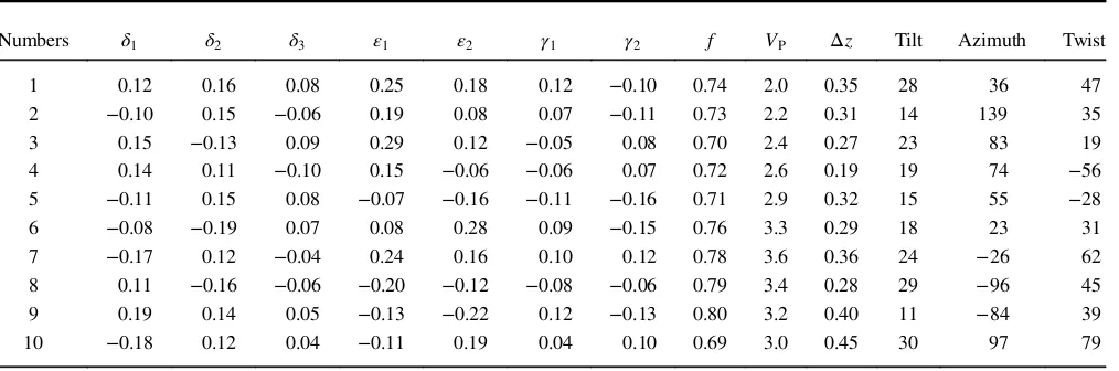
To determine the 21 interval stiffness matrix components, we

de-fine the layers as TOR, whose properties are presented in Table1. We

then transform (rotate) the local orthorhombic stiffness matrices into

the global frame (Bond, 1943). The data for each layer include the

layer thickness, nine orthorhombic elastic parameters, and the three Euler orientation angles: tilt, azimuth, and twist. The tilted frame is obtained from the global frame by three sequential rotations with

re-spect to theZY0_Z0 0_{axes, where the rotation angles are azimuth, tilt,}

and twist, respectively. The elastic properties include the

compres-sional velocityVPalong the tilted (local“vertical”) axisx3, the shear

parameterf¼1−V2S;x1∕V

2

P, whereVS;x1 is the velocity of S-waves

propagating along the local axisx3and polarized along the local axis

x1, and seven anisotropy parametersðδ1;δ2;δ3;ε1;ε2;γ1;γ2Þ

intro-duced by Tsvankin (1997), which are extensions of Thomsen’s

(1986)parameters for transverse isotropy.

The compressional velocity is in kilometers per second, the layer thickness is in kilometers, and the orientation angles (tilt, azimuth, and twist) are in degrees. For all layers, the tilt angle of the local vertical axis does not exceed 30°.

In Figure2, we plot the normalized second- and fourth-order

NMO velocities and the effective anellipticity versus slowness azi-muth and offset aziazi-muth. The NMO velocities are normalized by the average normal-incidence velocity. Note that the graphs of the fourth-order NMO velocities plotted for both azimuthal domains

show identical values at the azimuthsΨ2;LandΨ2;H, respectively.

For the second-order NMO velocities, these azimuths are common maximum and minimum points, whereas for the fourth-order velocities, these are just common points for the two domains.

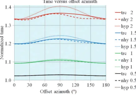
Figures3, 4, and5demonstrate the accuracy of the traveltime

approximation in the offset-azimuth domain. In Figure3, the

trav-eltime is plotted. For each plot, the offset is kept fixed, whereas the offset-azimuth runs from zero to 180°. The offsets are normalized,

¯

h_¼h∕z, wherezis the total thickness of the multilayer model. The

traveltimes are also normalized,¯t¼t∕to, wheretis the two-way

time andtois the two-way normal-incidence time (in this case, also

zero-offset time). Offsetsh¯ ≤2are considered.

Figure 2. Normalized second- and fourth-order global NMO veloc-ities (subplot a) and global effective anellipticity (subplot b) of the

multilayer TOR model from Table1in two azimuthal domains. The

labels“slw”and“off”denote slowness- and offset-azimuth domains,

respectively.

Figure 3. Ray-traced traveltime (solid lines) versus the hyperbolic (dotted lines) and nonhyperbolic (dashed lines) moveout approxi-mations in the offset-azimuth domain. Fixed offsets and varying off-set azimuth. Numbers in the legend show offoff-set-to-depth ratios.

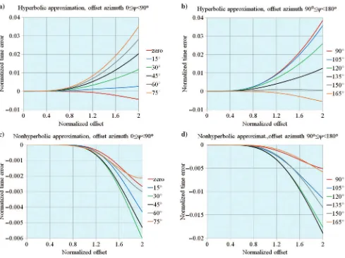
Figure4shows the absolute normalized traveltime errors in the offset-azimuth domain. The two-way traveltime error is divided by two-way normal incidence time. The offsets are kept fixed, whereas the offset-azimuth is changing. We show the errors of

the hyperbolic and nonhyperbolic approximations, for short and moderate offsets. For the maximum normalized offset considered,

¯

h¼2, the absolute normalized error of the hyperbolic

approxima-tion is approximately 0.039; for the nonhyperbolic approximaapproxima-tion,

Figure 5. Accuracy of the hyperbolic (subplots a and b) and nonhyperbolic (subplots c and d) moveout approximations in the offset-azimuth domain. Fixed offset azimuths and varying offset. Numbers in the legend show offset azimuths.

Figure 4. Accuracy of the hyperbolic (subplot a) and nonhyperbolic (subplot b) moveout approximations in the offset-azimuth domain. Fixed offsets and varying offset azimuth. Numbers in the legend show offset-to-depth ratios.

the maximum error is approximately 0.019. For shorter offsets, the

errors are much smaller. Figure5shows the same errors (hyperbolic

and nonhyperbolic approximations), but now we keep the offset-azimuth fixed, whereas the offset magnitude is changing. For mod-erate offsets, the nonhyperbolic term that depends on the fourth-or-der NMO velocity is crucial in achieving a reasonably accurate approximation.

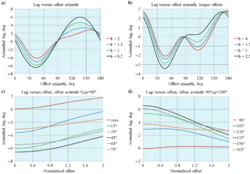
Figure6shows computed azimuthal lags (differences between

the offset-azimuth and slowness-azimuth) in the offset-azimuth

do-main,ΔΨðψoff; hÞ ¼ψoff−ψslw. In Figure6aand6b, the offset is

kept fixed, and the offset azimuth is changing. In Figure 6c

and6d, the offset azimuth is kept fixed, and the offset is changing.

The lags depend on the magnitude and azimuth of the offset vector, and they do not vanish even for zero-offset ray pair.

DISCUSSION OF GENERAL WORKFLOWS FOR ESTIMATING PARAMETERS OF AZIMUTHALLY

ANISOTROPIC MEDIA

Estimation of parameters of azimuthally anisotropic models is often performed as an iterative process in the depth-migrated domain (migration velocity analysis). Seismic migration is typically

performed with background velocity models, which are at first azi-muthally isotropic, e.g., VTI, and in later iterations, with azimu-thally anisotropic models. The latter include TTI and, possibly, other models of lower anisotropic symmetries, such as orthorhom-bic, TOR, monoclinic, tilted monoclinic, and triclinic. Due to azimuthally anisotropic effects, which are not included in the back-ground (migration) velocity models, reflection events in CIGs can show periodic azimuthally varying residual moveouts (RMO). The RMO can be estimated either by automatic event picking performed trace by trace, or by direct multiparameter search using explicit for-mulas for describing the RMO versus the perturbations of the global effective parameters (residual effective parameters). The RMO is obtained by taking the full differential of the NMO formula with respect to depth (or vertical time) and to the changes in the effective model parameters.

Furthermore, the coefficients of the RMO series expansions con-tain the global effective parameters of the background anisotropic velocity models, and therefore need to be directly calculated (for-ward Dix-type summation). Note that this is the main topic of this study. Both RMO representations (trace-by-trace and parametric) can be used as input for ray-based seismic tomography, which is the most commonly used method for globally updating the interval

Figure 6. Lags between offset and slowness azimuths in the offset-azimuth domain (computed exactly). Subplots a and b show fixed offsets and varying offset azimuth. Subplots c and d show fixed offset azimuths and varying offset. Numbers in the legends of the upper and lower subplots show offset-to-depth ratios and offset azimuths, respectively.

model parameters. In many cases, however, an intermediate approximate method is also used, which is based on the general Dix-type approach for local 1D models. In this case, first the updated local effective parameters at each layer are obtained from the updated global effective parameters, and then the local effective parameters are converted to interval parameters using some geo-logic and geophysical constraints.

A similar workflow for updating orthorhombic layered models

with only second-order RMO formula was proposed by Koren

and Ravve (2014).

CONCLUSION

We derive explicit expressions for slowness- and offset-azimuth domain NMO series coefficients of pure and converted modes in horizontally layered triclinic media. The accuracy of the NMO series expansions holds for leading error terms of order six. For pure-mode waves, the effective moveout parameters include the zero-offset time, three second-order, and five fourth-order coefficients. Alternatively, we propose an intuitive set of normalized parameters for pure modes with feasible ranges. This set includes the zero-offset time, two parameters describing the azimuthally invariant components of the moveout (second-order NMO velocity and effective anellipticity), and six residual parameters characterizing the azimuthal moveout variations. We further show that for weak azimuthal anisotropy, the second- and fourth-order NMO velocity functions in the off-set-azimuth domain reduce to simpler expressions in the slowness-azimuth domain. For converted waves, the odd (first-, third-, and fifth-order) coefficients of the NMO series are also required.

Forward computation of the local effective parameters requires explicit expressions for the near normal-incidence slowness surface and the derivatives of the vertical slowness with respect to the hori-zontal-slowness vector. We explicitly obtained all local effective parameters for each wave type as functions of the 21 stiffness co-efficients.

To check the validity of the analytic results, the nonhyperbolic traveltime approximation has been computed with the derived off-set-azimuth domain second-order NMO velocity and effective anel-lipticity. Comparison of this approximation and traveltimes computed for P-waves by numerical ray tracing in a horizontal, 10-layer TOR model shows a reasonable match for short and mod-erate offsets.

ACKNOWLEDGMENTS

The authors are grateful to Paradigm Geophysical for the finan-cial and technical support of this study and for permission to publish

its results. Gratitude is extended to the associate editor of G

EOPHYS-ICSI. Tsvankin and to the reviewers Y. Sripanich and R. Felicio Fuck

for constructive remarks and suggestions that helped to improve this paper.

APPENDIX A

NEAR NORMAL-INCIDENCE SLOWNESS SURFACE IN A TRICLINIC LAYER

In this section, we explicitly derive the general slowness surface expression in a triclinic layer in the proximity of the normal-incidence direction. We start with a general formulation for any

horizontal-slowness values; we then provide a series expansion sol-ution for small horizontal slowness (near normal-incidence rays).

The vertical slownessp3¼qðp1; p2Þcan be obtained by solving

the Christoffel equation

det_ðΓ−I_{Þ ¼}0; (A-1)

whereIis the identity tensor of order two and dimension three, and

Γ¼pCpis the second-order symmetric tensor with the given

co-efficients (e.g.,Slawinski, 2015)

Γ11¼C11p21þC66p22þC55p23

þ2_ðC16p1p2þC56p2p3þC15p1p3Þ; Γ_22¼C₆₆p2_1þC₂₂p2_2þC₄₄p2₃

þ2_ðC26p1p2þC24p2p3þC46p1p3Þ; Γ33¼C55p21þC44p22þC33p23

þ2ðC₄₅p₁p_2þC₃₄p₂p_3þC₃₅p₁p_3Þ; Γ12¼C16p21þC26p22þC45p23þ ðC12þC66Þp1p2

þ ðC_25þC_46Þp₂p_{3þ ð}C_14þC_56Þp₁p₃; Γ13¼C15p21þC46p22þC35p23þ ðC14þC56Þp1p2

þ ðC_36þC_45Þp₂p_{3þ ð}C_13þC_55Þp₁p₃; Γ23¼C56p21þC24p22þC34p23þ ðC25þC46Þp1p2

þ ðC23þC44Þp2p3þ ðC36þC45Þp1p3: (A-2)

The vanishing determinant in equation A-1results in 950

mono-mials (items). However, we collect them into 50 coefficients

corresponding to the specific combinations of powers pi

1p j 2pk3.

EquationA-1may be arranged as a sixth-order polynomial equation

that makes it possible to obtain the vertical-slowness component

p3¼qðp1; p2Þfrom the horizontal componentsp1andp2

A6q6þA5q5þA4q4þA3q3þA2q2þA1qþA0¼0; (A-3)

where Ak are the polynomials of degree6−kversusp1and p2.

Their coefficients, in turn, depend only on the density normalized

stiffness matrix components Cij; i; j¼1; : : : ;6. Hence, A6 is a

constant, A5 is a linear polynomial of the horizontal slowness,

A4 is a quadratic polynomial, etc. The coefficients of

equa-tionA-3, A0: : : A6, are explicitly listed in AppendixB. Because

they are polynomials ofp1andp2, their derivatives with respect

to p1 and p2 can be easily obtained. The six roots of

equa-tionA-3can be split into three pairs, in which each pair corresponds

to P-, fast S-, and slow S-waves. The two roots of each pair corre-spond to the downgoing and upgoing modes. In this paper, for the sake of symmetry, both rays of the incidence-reflection ray pair are considered to emerge up from the reflection point; thus, we deal only with upgoing rays. The positive vertical direction is assumed

upward. Because the slowness surface presented by equationA-3is

implicit, we have to first solve the sixth-order polynomial equation and only then select the proper root. We approximate the vertical

slowness by an explicit functionp3¼qðp1; p2Þfor small

horizon-tal-slowness components. For the vertical slowness vector, we

troducep1¼p2¼0into equationA-2, and the Christoffel matrix of a triclinic medium simplifies to

Γ¼

and its eigenvalues are the vertical phase velocity squared, vver_phs¼q−1

o . The subscript zero refers to the normal-incidence

direc-tion (zero horizontal slowness). We can also compute the

coeffi-cients Ao₀: : : Ao₆ corresponding to the normal-incidence ray (see

AppendixB). Now consider a ray in the vicinity of the

normal-in-cidence direction, in which the horizontal slownessphis finite but

small. The polynomial coefficients change slightly

A6¼Ao6;

m;n denotes a symmetric tensor of ordernand dimension

two for thenth derivatives of the coefficientAm, with respect top1

andp2, computed for the normal-incidence direction. All

compo-nents of these tensors can be obtained in a straightforward manner

from the relationships listed in AppendixB. The dot sign means a

full scalar product; for example,

Ao_0;4·p4_{h ¼} ∂

Following equation1, computation of the ray-velocity components

includes a differential operator that reduces the polynomial degree, and thus the accuracy of the approximation. Therefore, to achieve the fourth-order accuracy for the ray-velocity components that af-fects one-way kinematic parameters, we need the fifth-order accu-racy for the slowness surface.

Similarly to the polynomial coefficientsAo₀: : : Ao₆ (equation set

A-5), the vertical slownessqðp1; p2Þ may also be expanded into

a series in the proximity of the normal-incidence ray (see equation4,

in which all derivatives correspond to the normal-incidence

direc-tion). Unlike the derivatives of the polynomial coefficientsAom;n, the

tensor derivatives of the vertical slownessqnare unknown and have

to be found. For this, we substitute equations 4andA-5into the

Christoffel-based polynomial equation A-3. We ignore the higher

order termsO_ðp6_{hÞ, and we then balance the terms with the same}

powers of horizontal slowness. All the derivative tensors may be presented as

where q¯n is a symmetric tensor of order n and dimension two,

whose components are proportional toqn. We callq¯nthe

normal-ized derivative tensors (although they are not dimensionless). The

denominator in equationA-7is a scalar (just a scaling factor). It

follows from Appendix Bthat for the normal-incidence ray only

even-order coefficients of the polynomial are nonzero for the

nor-mal-incidence direction, and equationA-7simplifies to

qn¼−

Given the two componentsp1andp2of the horizontal-slowness

vector, the vertical slownessqðp1; p2Þmay be obtained from the

Christoffel equation, expressed by the six-order polynomial

equa-tionA-3. The coefficients read

A_6¼2C₃₄C₃₅C_45þC₃₃C₄₄C₅₅