Long-term record of atmospheric CO
2and stable isotopic ratios
at Waliguan Observatory:
Background features and possible drivers, 1991–2002
Lingxi Zhou,1 Thomas J. Conway,2 James W. C. White,3 Hitoshi Mukai,4 Xiaochun Zhang,1 Yupu Wen,1 Jinlon Li,5 and Kenneth MacClune3
Received 8 December 2004; revised 28 June 2005; accepted 10 July 2005; published 14 September 2005.
[1] This paper describes background characteristics of atmospheric CO2 and stable
isotopic ratios (d13C and d18O) as well as their possible drivers at Waliguan Baseline Observatory (WLG) (36170N, 100540E, 3816 m above sea level) in the inland plateau
of western China. The study is based on observational CO2 data (NOAA Climate
Monitoring and Diagnostics Laboratory discrete and WLG continuous measurements) obtained at WLG for the period from May 1991 to December 2002. Over this period the change in monthly means is +16 ppm for CO2,0.2% for d13C, and 0.5%
ford18O. The overall increase of CO
2 and subsequent decline ofd13C, with a
Dd13C/DCO2ratio (0.011 ± 0.105)% ppm1at WLG, reflect the persistent worldwide
influence of fossil fuel emissions. The negative secular trend ofd18O at WLG is probably due to vigorous18O exchange with soils in the Northern Hemisphere (NH) and
conversion from C3 to C4 plants via land use change. The CO2,d13C, andd18O mean
annual cycles with peak-to-peak annual amplitudes of10.5 ppm, 0.499 %, and
0.819%, respectively, at WLG show typical middle-to-high NH continental features
that correspond to the seasonal cycle of the terrestrial biosphere. The significant CO2and d13C interannual variability at WLG is very likely caused by worldwide climate
anomalies and associated regional fluctuation in biospheric CO2uptake in the Asian
inland plateau as well as long-range air mass transport. The results of this study help to provide a basic understanding of the individual sources and sinks of carbon in this area and help us to better address the role of the Asian inland terrestrial biosphere in the global carbon cycle.
Citation: Zhou, L., T. J. Conway, J. W. C. White, H. Mukai, X. Zhang, Y. Wen, J. Li, and K. MacClune (2005), Long-term record of atmospheric CO2and stable isotopic ratios at Waliguan Observatory: Background features and possible drivers, 1991 – 2002,
Global Biogeochem. Cycles,19, GB3021, doi:10.1029/2004GB002430.
1. Introduction
[2] CO2 fluxes at the Earth’s surface include respiration
and photosynthesis of the terrestrial biosphere, exchange with the oceans, and anthropogenic sources such as fossil fuel combustion and land use changes. Since the eighteenth century, increasing emissions of anthropogenic CO2 have
been distributed among the reservoirs of CO2. About half of
the CO2 released into the atmosphere by human activity
remains there, with the other half absorbed either by the land biosphere or the oceans [Andres et al., 1996;Pearman and Hyson, 1986; World Meteorlogical Organization
(WMO), 2003]. Long-term observation of the atmospheric CO2 mixing ratio and d13C from a globally distributed in
situ and discrete air sampling network can enable the determination of source/sink variability and allow quantita-tive partitioning of fluxes into terrestrial and oceanic reser-voirs because these exchange paths influence CO2isotopes
in different ways [Ciais et al., 1995a, 1995b;Francey et al., 1995; Nakazawa et al., 1993, 1997a, 1997b; Tans et al., 1990;Trolier et al., 1996]. Additionally,d18
O measurements allow the separation of terrestrial net ecosystem production (NEP) into its photosynthetic and respiratory components on the basis of their contrasting effects on the d18O of atmospheric CO2[Ciais et al., 1997a, 1997b; Flanagan et al., 1997; Ishizawa et al., 2002; Miller et al., 1999]. The CO2 mixing ratio and isotope measurements can also be
used in studies of natural variability in the carbon cycle and 1Key Laboratory for Atmospheric Chemistry, Centre for Atmosphere
Watch and Services, Chinese Academy of Meteorological Sciences, China Meteorological Administration, Beijing, China.
2
Climate Monitoring and Diagnostics Laboratory, NOAA, Boulder, Colorado, USA.
3
Institute for Arctic and Alpine Research, University of Colorado, Boulder, Colorado, USA.
4
Center for Global Environmental Research, National Institute for Environmental Studies, Tsukuba, Japan.
5
School for Environmental Sciences, Peking University, Beijing, China.
in calibrating global carbon budget models [Heimann and Maier-Reimer, 1996; Keeling et al., 1989a, 1989b, 1995;
Tans et al., 1989, 1996].
[3] The measurements from various global monitoring
networks together with modeling studies have identified the northern midlatitude terrestrial biosphere as a major component of the ‘‘missing sink.’’ However, spatial cov-erage of the existing networks is still too sparse to be able to reach satisfactory conclusions with respect to specific fluxes, especially in midcontinental regions where it is likely that important carbon sources and sinks are located [Bakwin et al., 1998; Francey et al., 1998; Houghton et al., 1998;Levin et al., 1995;Miller et al., 2003;Morimoto et al., 2000]. Waliguan Baseline Observatory (WLG)
(36170N, 100540E, 3816 m above sea level), situated in
remote western China, is one of the World Meteorological Organization’s (WMO) 22 Global Atmosphere Watch (GAW) baseline stations scattered around the globe. The locations of the GAW baseline stations are mostly coastal (http://www.wmo.ch/web/gcos/gif/gaw.gif) [WMO, 1993, 2001, 2003; World Data Center for Greenhouse Gases
(WDCGG), 2003]. Funded by the United Nations and the Chinese Government, WLG was officially opened in 1994 by the China Meteorological Administration as China’s first long-term research station for the continuous moni-toring of greenhouse gases, ozone, aerosols, and meteo-rology [Wen et al., 1994;Zhou et al., 2003]. Because of its unique location the measurements from WLG provide essential information on sources and sinks from within the Eurasian continent, and they have received attention in recent years [Climate Monitoring and Diagnostic Laboratory (CMDL), 2004; Masarie and Tans, 1995;
Miller et al., 2003; WMO, 2003; WDCGG, 2003] (see also http://www.cmdl.noaa.gov/ccgg/globalview).
[4] In this study, the monthly mean time series, secular
trend, annual cycle, and interannual variability of atmo-spheric CO2and stable isotopic ratios observed at WLG are
presented and characterized. The results from WLG show specific features that will provide additional constraints for atmospheric models to help improve the understanding of atmospheric CO2and the global carbon cycle, particularly
over the Asian inland plateau.
2. Site and Experiment
2.1. Sampling Site
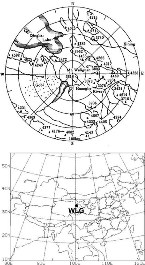
[5] Figure 1 shows the geographical location and
topog-raphy of the area (100 km radius) around Mount Waliguan (WLG). Located at the edge of the northeastern part of the Tibetan Plateau, the area surrounding the WLG station is essentially untouched, maintaining its natural environment of sparse vegetation along with arid and semiarid grassland and some desert regions. Yak and sheep grazing is the main activity during summer (June, July, and August), with small agricultural regions located in the lower valley area. The population density is less than 6 people km2
, and the station is relatively isolated from industrial and populated centers.
2.2. Discrete Measurements
[6] In 1991 the National Oceanic and Atmospheric
Administration Climate Monitoring and Diagnostic Labo-ratory (NOAA CMDL) began a weekly air sampling program at WLG. Two samples are collected in series from 5 m above ground using glass flasks and a portable battery-powered sampling apparatus (flushing and then pressurizing glass flasks with a pump). The discrete air samples collected at WLG are measured for CO2 (and other trace
gas species) by a nondispersive infrared (NDIR) analyzer at the NOAA CMDL Carbon Cycle Greenhouse Gases group in Boulder, Colorado, USA. Measurement precision for CO2determined from repeated analysis of the same air
is0.1 ppm. The isotopic measurements of the discrete air samples are performed at the Stable Isotope Laboratory of
the Institute for Arctic and Alpine Research of the Uni-versity of Colorado. A Micromass Optima dual inlet isotope ratio mass spectrometer achieves overall reproduc-ibility of ±0.01% for d13
C and ±0.03% for d18
O. The monthly means from the discrete samples are produced by first averaging all valid measurement results with a unique sample date and time, then extracting values at weekly intervals from a smooth curve fitted to the averaged data and averaging these values for each month to give the monthly means (http://www.cmdl.noaa.gov/ccgg/iadv/). Descriptions of the sampling, measurement, standards, calibration procedures, curve fitting, analysis, and inter-pretation of the CO2and isotopes (d13C and d18O) data are
given in other works [Conway et al., 1994;Thoning et al., 1989; Trolier et al., 1996].
2.3. In Situ Continuous Measurements
[7] The main building housing the WLG in situ CO2
measurement systems and an 89-m triangular steel tower for ambient air sampling (80 m) is located at the top of Mount Waliguan. The atmospheric CO2 mixing ratios were
mea-sured using a Licor6251 NDIR analyzer and a HP5890 gas chromatograph (GC) equipped with a flame ionization detector (FID). The NDIR system began in November 1994 with an ambient analysis frequency of one per minute. The GC-FID system began in July 1994 with 64 ambient injections per day (CO2 converted to CH4 by a nickel
catalyst tube heated to 350). The overall precision of the NDIR and the GC-FID analyses is below 0.02% and 0.05%, respectively, from repeated analysis [Wen et al., 1994;Zhou et al., 1998]. The standard scale employed by the WLG in situ CO2measurements is tied to the NOAA CMDL CO2
measurement scale and compared through periodic inter-comparison experiments (see http://www.cmdl.noaa.gov/ ccgg/globalview). The CO2monthly means from the in situ
NDIR and GC-FID measurements are integrated (to reduce data gaps) from the selected hourly data representative of background atmospheric conditions. The system configura-tions and routines, CO2 standard gases and reference
scale, intercomparison experiments, calibration and quality control, impact of local winds and long-range transport on the continuous CO2 record, background data filtering and
merging methodology, etc., are described in previous studies [Zhou, 2001; Zhou et al., 2003].
2.4. Measurement Scale and Observational Data
[8] In this paper, the CO2 mixing ratios are reported on
the NOAA CMDL measurement scale [CMDL, 2004] (see also http://www.cmdl.noaa.gov/ccgg/globalview) in units of mmol mol1
(106
mol CO2 per mol of dry air). The
isotopic ratios are expressed in per mil (%) relative to the
standard isotopic ratio Vienna Peedee belemnite CO2
[Trolier et al., 1996] for both d13C andd18O.
[9] A total of 118 monthly mean CO2values (May 1991
to December 2002, NOAA CMDL network) were derived from the discrete samples. A total of 84 monthly mean CO2
values (August 1994 to December 2002, WLG in situ measurements) were extracted using continuous data. A comparison of the overlapping (62 months) discrete and continuous monthly mean CO2 data resulted in a mean
difference (±2s, discrete minus continuous) of (0.59 ± 0.23) ppm. One possible reason for this difference is the different air sampling heights (5 m above ground for discrete and 80 m for continuous measurement). The CO2 monthly means at WLG over the entire period from
May 1991 to December 2002 (140 months in total) used in this study are merged from all of the continuous and discrete air sample measurements. The monthly means of the d13
C (120 months) and d18
O (110 months) at WLG over the entire period were derived from the discrete samples. The CO2 and isotope data from the discrete
samples from November 1994 to June 1996 are rejected because a sampling malfunction contaminated the samples.
3. Results and Discussion
3.1. Atmospheric CO2,D13C, andD18O
Monthly Mean Time Series
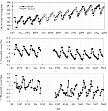
[10] Monthly mean atmospheric CO2mixing ratios,d13C,
and d18
O at WLG from May 1991 to December 2002 are shown in Figure 2. The CO2 andd13C monthly data vary
seasonally. The CO2 data showed typical spring maxima
and summer minima. The d13
C data showed an opposite annual cycle that is almost a mirror image to that of the CO2. The d18O monthly data exhibited relatively large
scatter with annual maxima that occurred mostly in June (early summer at WLG).
[11] The overall change of the mean mixing ratio is
+16 ppm for CO2,0.2% ford13C, and0.5% for d18
O. It is well known that the secular increase of atmo-spheric CO2 mixing ratio and decline of d13C are mainly
driven by fossil fuel combustion and terrestrial deforesta-tion, which add carbon with low isotopic ratios to the atmosphere. The CO2andd13C trends are also affected by
uptake and release of CO2from the oceans and terrestrial
biosphere. Though less addressed than d13
C, the d18
O of atmospheric CO2contains information about both plant and
soil respiration in addition to plant photosynthesis. Gillon and Yakir[2001] suggested that the recent observed decline ofd18
O in atmospheric CO2(0.02%yr1) is partly due to
the conversion of C3 forest to C4 grasslands via land use
change. Ciais et al. [1997b] suggested that vigorous 18O exchange with soils is primarily responsible for the persis-tent depletion ind18
O over the high latitudes of the Northern Hemisphere (NH), while leaf isotopic exchange opposes this effect in the NH.Ishizawa et al.[2002] speculated that the recent d18
O downward trend (0.5% yr1
from Northern Hemisphere to Southern Hemisphere for the period from 1993 to 1997) is mainly caused by enhanced photosynthetic activity in the NH. The observed decline of
d18
O in atmospheric CO2 at WLG (0.5% from May
1991 to December 2002) is consistent with the above mentioned viewpoints and is likely caused by active 18O exchange with soils in this region of the NH.
3.2. Atmospheric CO2andD13C Annual Means,
Growth Rates, and Interannual Variability 3.2.1. Annual Means and Growth Rates
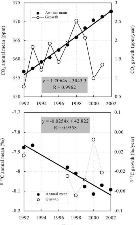
[12] Annual means (derived from monthly means within
rates (estimated incremental value in each year) of the atmospheric CO2 mixing ratio and d13C at WLG from
1992 to 2002 are shown in Figure 3. The d13C annual means and growth rates in 1994, 1995, and 1996 are missing because of large data gaps (no data available from November 1994 to June 1996 due to sampling malfunction). Thed18O annual means (growth rates as well as interannual fluctuations) have not been computed and discussed because of frequent data gaps within most of the years and the large scatter of the monthly data.
[13] The CO2 annual means vary from 356.65 ppm
(minimum in 1992) to 372.65 ppm (maximum in 2002) and increase approximately linearly with a 10-year average (±2s) mean growth rate of 1.60 ± 0.38 ppm yr1
from 1992 to 2002. The d13C annual means vary from 7.867%
(heaviest in 1993) to 8.115% (lightest in 2000) and
decrease almost linearly with a 10-year average (±2s) mean decrease rate of 0.017 ± 0.040% yr1
. The 10-year average (±2 s) mean ratio of the secular trends from 1992 to 2002 (Dd13
C/DCO2) is calculated to be (0.011 ±
0.105)% ppm1
. The ratio observed at WLG is much higher than the Dd13
C/DCO2 ratios of 0.030 to
0.020% ppm1 [Keeling et al., 1979; Mook et al., 1983; Nakazawa et al., 1993, 1997a, 1997b] observed from other background tropospheric measurements during previous time spans. Additionally, the ratio at WLG is higher than the global average ratio of 0.021%ppm1
estimated a decade ago by using a two-dimensional (2-D) transport model [Pearman and Hyson, 1986] and is close to ratios of 0.015 to 0.011% ppm1
at La Jolla, Mauna Loa, Fanning-Christmas Islands, and the South Pole deduced from a 3-D transport model [Keeling et al., 1989a]. On the basis of other studies [Ciais et al., 1995a, 1995b, 1999; Miller et al., 2003; Nakazawa et al., 1993, 1997a, 1997b;Still et al., 2003] the averageDd13C/ DCO2 ratio at WLG is much higher than the rate of
0.05% ppm1
expected for the short-term fossil fuel combustion sources or discrimination by C3 plants. It is,
however, lower than the 0.005% ppm1
expected from short-term oceanic CO2 sources and close to the
Figure 2. Monthly mean atmospheric CO2mixing ratios,d13C, and d18O at WLG from May 1991 to
December 2002. The solid circles represent CO2,d13C, andd18O monthly means, respectively, from the
0.01% ppm1
from short-term discrimination by terres-trial C4 plants. We postulate that the average changing
ratio at WLG is due to the initial CO2 released into the
atmosphere by fossil fuel combustion and deforestation exchanging and equilibrating between the atmosphere-biosphere and the atmosphere-oceans over a 10-year timescale, during which the isotopic signal is diluted faster than that of the original CO2emitted into the atmosphere.
The fast equilibration during short-term CO2 exchange
along with isotopic disequilibrium could affect the final isotopic value of the atmosphere that is measured and the interannual variations.
3.2.2. Interannual Variability
[14] The CO2growth rates from 1992 to 2002 vary from
0.77 ppm yr1
(minimum in 1992 and a notable low value 0.99 ppm yr1
in 2000) to 2.52 ppm yr1
(maximum in
1998), showing significant interannual variability. Thed13
C growth rates from 1992 to 2002 vary from 0.069%yr1
in 1998 to 0.044% yr1
in 2000, showing significant interannual changes.
[15] On the basis of numerous other studies [Andres et al.,
1996; Ciais et al., 1999; Conway et al., 1994; Francey et al., 1990, 1995, 1998;Keeling et al., 1989a, 1989b, 1995;
Morimoto et al., 2000; Nakazawa et al., 1993, 1997a, 1997b;Trolier et al., 1996; Watanabe et al., 2000; WMO, 2003; Zahn et al., 2000] we summarized that the atmo-spheric CO2 mixing ratio is highest in northern high and
midlatitudes reflecting strong net sources in these areas, with a North Pole minus South Pole gradient of 3 ppm. The high global growth rates in 1983, 1987/1988, 1994/ 1995, and 1997/1998 are associated with warm El Nin˜o – Southern Oscillation (ENSO) events. The anomalously strong El Nin˜o event in 1997/1998 brought about a record high growth rate in 1998. The exceptionally low growth rate in 1992 was caused by the low global air temperatures following the eruption of Mount Pinatubo in 1991. The observed trend in globally averaged CO2is1.6 ppm yr
1
during last the 2 decades. The North Pole minus South Pole
d13C gradient is0.3%, driven primarily by isotopically
light excess fossil fuel CO2being preferentially released in
the Northern Hemisphere. The rate of decrease in thed13C is enhanced in the years corresponding to larger increases in CO2. The observed trend ind
13
C during the last 2 decades averaged0.025%yr1
, and a more persistent flattening was observed globally beginning in 1988 – 1992, most likely as a result of increased net uptake by the terrestrial biosphere.
[16] Biospheric model studies predict that plant
respira-tion and soil decomposirespira-tion are enhanced in ENSO years by above-average temperatures and precipitation, which leads to a reduction in net CO2 uptake by the terrestrial
biosphere [Kindermann et al., 1996; Ito and Oikawa, 2000]. A recent model calculation [Cao et al., 2003] on the interannual variations and trends in terrestrial carbon uptake caused by climate variability in China during the period of 1981 – 1998 indicated that both temperature and precipitation reached the highest value in 1998, a record for the twentieth century, and resulted in the largest soil heterotrophic respiration (HR) in arid northwest China where WLG is located. In 1992, however, both tempera-ture and precipitation reached the lowest values.Cao et al.
[2003] also suggested that in arid northwest China, HR varied with changes in temperature, but its correlation with precipitation was not significant. For instance, in another warm but dry year, 1997 the HR increased significantly in northeast and southwest China, but it had no increase in arid northwest China.
[17] It is well known that CO2 exchange between the
atmosphere and oceans or between the atmosphere and terrestrial C4 plants produces only minor change in
atmo-sphericd13C. The interannual variation of atmospheric CO2
andd13
C trends observed at WLG is very likely caused by worldwide climate variability (e.g., El Nin˜o) and associated variability in biospheric uptake (including changing C3/C4
composition caused by land use activities). The maximum CO2 increase along with a maximum d13C decrease
Figure 3. Annual means (solid circles) and growth rates (open circles and thin lines) of the atmospheric CO2mixing
observed at WLG in 1998 represented the least amount of carbon entering the biosphere during the period from 1992 to 2002. The lower CO2 and d
13
C trends at WLG since 1999 indicate that more carbon has been entering the biosphere since then. The exceptional rises in the d13C in atmospheric CO2during the periods 1992 to 1993 and
2000 to 2001 observed at WLG indicate large land sinks for carbon during those years.
3.3. Atmospheric CO2,D13C, andD18O Mean Annual
Cycles and Year-to-Year Changes
3.3.1. Constructing Detrended Monthly Data
[18] A monthly mean time series of the atmospheric CO2
mixing ratio or isotopes, which is often produced by removing local effects with very short term variation, is an integration of variation on different timescales, such as annual cycle, secular trend, and interannual variation. According to several studies [Denning et al., 1995; Levin et al., 1995; Randerson et al., 1997, 2002; Trolier et al., 1996; WMO, 2003], to investigate mean annual cycle features or the relationship between seasonal changes of
the atmospheric CO2 and isotope ratios, secular trends
should first be removed. In this paper, all the detrended monthly data have been constructed by simply subtracting a linear secular trend from each of the monthly mean time series.
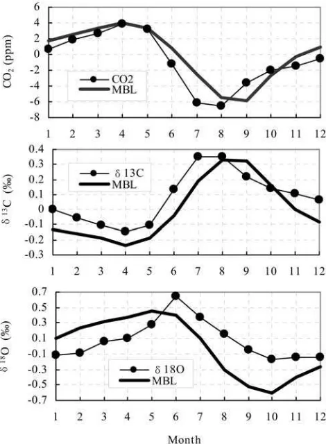
3.3.2. CO2,D13C, andD18O Mean Annual Cycles [19] The atmospheric CO2,d13C, andd18O mean annual
cycles at WLG for the period from May 1991 to December 2002 are shown in Figure 4. Each of the mean annual cycles was constructed by separately averaging all avail-able data in the detrended monthly mean time series to get a mean value for each month. Also shown are the annual cycles for the marine boundary layer (MBL) reference (see http://www.cmdl.noaa.gov/ccgg/globalview) for the same latitude.
[20] The CO2mean annual cycle at WLG has a maximum
in April and minimum in August, declining rapidly during the May – July growing season and climbing slowly during September – November. The peak-to-peak annual amplitude is10.5 ppm. The CO2minimum in the mean annual cycle
occurred almost a month earlier than in the MBL reference (MBL maximum in April and minimum in September, peak-to-peak amplitude of 9.8 ppm). The phasing of the
d13
C mean annual cycle is opposite to that of CO2. The
lowestd13C values occurred at the beginning of the growing season in April, and the highest occurred at the end of the growing season in August. This reflects the seasonality of terrestrial vegetation growth in the middle to high latitudes of the NH. The peak-to-peak annual amplitude is0.499%.
The d13
C maximum and minimum occurred in the same months as in the MBL reference (MBL peak-to-peak amplitude 0.570%). A similar relationship between the
phase of the seasonal cycles of d13C and CO2 has been
observed at other locations in the NH troposphere. These studies [Nakazawa et al., 1993, 1997a, 1997b;Friedli et al., 1987;Mook et al., 1983;Keeling et al., 1984, 1989a;Trolier et al., 1996] indicated that the strong seasonality of atmo-spheric CO2andd13C in the NH is mainly due to exchange
of CO2 between vegetation and the atmosphere, i.e.,
pho-tosynthesis and respiration of the terrestrial biosphere throughout the year, in which photosynthesis is dominant in the warm season and respiration exceeds photosynthesis in the cold season.
[21] The d18O mean annual cycle at WLG is maximum
in June, then decreases sharply during July – September to reach a minimum in October. The peak-to-peak annual amplitude is 0.819%. The d18O maximum in the mean annual cycle at WLG occurred nearly a month later than the MBL reference (MBL maximum in May and minimum in October, peak-to-peak amplitude of 1.05%). The lag
of the d18O in the mean annual cycle versus CO2
maxi-mum and minimaxi-mum at WLG is 2 months, comparable to the results obtained at Barrow, Alaska (BRW) (71N, 63W) from observations [Trolier et al., 1996] and model simulation [Ciais et al., 1997b]. An interpretation of the seasonal d18O variation is much more difficult than for the d13C and the CO2mixing ratio. This is due to complicated
combinations of different seasonally varying fluxes of biospheric CO2in the atmosphere and the various
weather-dependent factors (e.g., solar radiation, temperature,
pre-Figure 4. Atmospheric CO2,d13C, andd18O mean annual
cycles at WLG from May 1991 to December 2002. The circles and thin lines are derived from the detrended CO2, d13
C, andd18
cipitation, etc.) governing the d18
O composition in CO2
[Nakazawa et al., 1997b]. Ciais et al. [1997b] indicated that in the NH the influence of soil respiration explains the observed phase lag of d18O versus CO2. The October –
November minimum in d18
O at the high-latitude NH site BRW is due to isotopic exchange with soils as the dominant component of the seasonal cycle. However, canopy exchange contributes proportionally more to the seasonality of d18
O at the lower-latitude NH site Mauna Loa, Hawaii (MLO) (20N, 155W) than at BRW because leaf isotopic exchange causes an increase in d18
O during July – August at MLO, so that d18O at MLO reaches maximum in June – July and minimum in September – October. The lag of the d18O versus CO2 minimum at
MLO is less than a month. On the basis of the above statements the measured d18O seasonal cycle in atmo-spheric CO2at the middle- to high-latitude NH site WLG
was mainly caused by the latitudinal-dependent d18O of precipitation and thus soil water.
3.3.3. CO2andD 13
C Annual Cycle Amplitude Variations
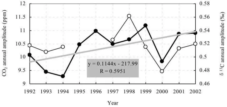
[22] Interannual variations in the seasonal cycle of
atmo-spheric CO2andd13C at WLG for the period of 1992 – 2002
are shown in Figure 5. The CO2 and d13C annual cycle
amplitudes are derived from detrended monthly data points within each year (maximum minus minimum, i.e., peak to peak). The d18
O annual cycle amplitude interannual varia-tion has not been computed and discussed because of large data gaps and scatter within most of the years.
[23] During the period from 1992 to 2002 the CO2annual
cycle amplitude reached the highest value, 11.2 ppm, in 1999 and the lowest value, 9.3 ppm, in 1994. The 11-year average (±2s) mean annual amplitude is calculated to be (10.4 ± 0.4) ppm. Except for the year 2000 the amplitudes for 1995 – 2002 are all larger than for 1992 – 1994. Thed13
C annual cycle amplitude reached a maximum of 0.562% in
1998 and a minimum of 0.479% in 2000. There are no
annual amplitude data for the years 1995 and 1996. The
interannual variations in d13
C tend to track those of CO2.
The period of 1998 – 1999 is an exception, with an amplitude increase in CO2 and a decrease in d13C. The
period of 1993 – 1994 is another exception, with an amplitude decrease in CO2 and an increase in d13C. The
9-year average (±2s, 1992 – 1994 and 1997 – 2002) annual amplitude is (0.517 ± 0.016)%.
[24] The interannual variability in the CO2 and d13C
seasonal cycles is due to variations in the seasonal balance between photosynthesis and respiration, as well as seasonal oceanic fluxes and atmospheric transport. In the NH middle and high latitudes, interannual variations in the seasonal cycles are at least an order of magnitude smaller than their seasonal variations [Randerson et al., 1997; Zahn et al., 2000]. A study of the secular trend of the CO2 seasonal
amplitude from longer atmospheric CO2monitoring records
found that the seasonal amplitude in the NH had increased [Bacastow et al., 1985]. Other studies have shown that at stations north of 55N the atmospheric CO2 seasonal
amplitude increased at a mean rate of 0.66% yr1
from 1981 to 1995 [Randerson et al., 1997] and that the CO2
amplitude increased 20% at MLO (20N) from 1958 to 1994 and 40% at BRW (71N) from 1961 to 1994 [Keeling et al., 1996]. A similar trend was observed at Alert, Nunavut, Canada (ALT) (82N) during the 1980s [Conway et al., 1994]. Previous studies [Keeling et al., 1989a; Randerson et al., 1997] also speculated that the seasonal cycle of atmospheric CO2 at surface sites in
the NH is driven primarily by NEP, so the increase in the seasonal cycle amplitude suggests that NH terrestrial ecosystems are experiencing greater CO2 uptake during
the growing season and greater CO2 release during
periods outside the growing season. An increasing trend in the seasonal cycle amplitude is observed in the WLG atmospheric CO2 record for the period of 1992 – 2002
(0.1 ppm yr1
by a linear fit to the data shown in Figure 5) in agreement with results from NH sites. The year 2000 is an exception. The observed lower CO2 and
Figure 5. Year-to-year fluctuations of the annual cycle amplitudes for the atmospheric CO2mixing ratio
(solid circles and thick lines) and d13
d13
C annual cycle amplitudes are probably due to climate perturbations and associated variability in biospheric uptake.
4. Conclusions
[25] The WLG continuous in situ and NOAA CMDL
discrete air sample measurements of CO2mixing ratios at
WLG are in good agreement with a mean difference (0.59 ± 0.23) ppm for the overlapping monthly means. The in situ CO2 annual means vary from 356.65 to 372.65 ppm and
increase approximately linearly with a mean growth rate of (1.60 ± 0.38) ppm yr1
from 1992 to 2002. Thed13C annual means vary from7.867 to8.115%and decrease almost
linearly with a mean decline rate of (0.017 ± 0.040)%
icant interannual variability that is very likely caused by worldwide climate anomalies and associated changes in biospheric uptake. The maximum CO2increase along with
a maximumd13
C decrease at WLG in 1998 reflects the least amount of carbon entering the biosphere during this period. The minimum CO2increase and an abnormald13C increase
at WLG in 2000 suggest that more carbon is entering the biosphere.
[26] The mean CO2 seasonal cycle at WLG has a
maximum in April and a minimum in August. The CO2 minimum in the mean annual cycle occurred almost
1 month earlier than in the MBL reference at the same latitude. The peak-to-peak annual amplitudes vary irregu-larly from year to year but appear to have been increasing since 1995, except for the year 2000. The 11-year average mean annual amplitude is (10.4 ± 0.4) ppm. The phasing of thed13C mean annual cycle is opposite to that of CO2.
The d13
C maximum and minimum occurred in the same months as in the MBL reference. The d13C peak-to-peak amplitudes also vary from year to year. The 9-year average annual amplitude is (0.517 ± 0.016)%. The d18O mean annual cycle has a maximum in June and a minimum in October with peak-to-peak amplitude of 0.819%. The d18
O maximum in the mean annual cycle at WLG occurred nearly a month later than the MBL reference. The study presents an 11-year record of atmospheric CO2and stable
isotopes observed in this particular region. The results will contribute to a better understanding of the global carbon cycle, especially in the inland plateau of the Eurasian continent.
[27] Acknowledgments. This work is supported by a Key Project sponsored by the Scientific Research Foundation for the Returned Overseas Chinese Scholars (State Personnel Ministry [2004]99), a Climate Change Research Foundation (China Meteorological Administration CCSF2005-3-DH04), a Japan Society for Promotion of Science Post-doctoral Fellowship (PB01736), and a United Nations GEF Fund (GLO/91/G32). We thank the staff of Waliguan Station for their efforts in operating the continuous CO2 observing systems and collecting the flask air samples. We appreciate NOAA CMDL and CU-INSTAAR for cooperation on the Waliguan NDIR and flask air-sampling programs. MSC Canada is appreciated for the cooperation on the Waliguan GC-FID program. We also appreciate the WMO AREP Environment Division for the coordination of the GAW program. Helpful comments and suggestions of two anonymous reviewers are gratefully acknowledged. The authors would like to especially thank one of the reviewers: The annotated manuscript contributed to a significant
improvement in the resubmission and the further revised version of this paper.
References
Andres, R. J., G. Marland, I. Fung, and E. Matthews (1996), A 11
distribution of carbon dioxide emissions from fossil fuel consumption and cement manufacture, 1950 – 1990,Global Biogeochem. Cycles,10, 419 – 429.
Bacastow, R. B., C. D. Keeling, and T. P. Whorf (1985), Seasonal amplitude increase in atmospheric CO2concentration at Mauna Loa, Hawaii, 1959 – 1982,J. Geophys. Res.,90, 10,529 – 10,540.
Bakwin, P. S., P. P. Tans, J. W. C. White, and R. J. Andres (1998), Deter-mination of the isotopic (13C/12C) discrimination by terrestrial biology from a global network of observations,Global Biogeochem. Cycles,
12, 555 – 562.
Cao, M. K., S. D. Prince, K. R. Li, B. Tao, J. Small, and X. M. Shao (2003), Response of terrestrial carbon uptake to climate interannual variability in China,Global Change Biol.,9, 536 – 546.
Ciais, P., P. P. Tans, J. W. C. White, M. Trolier, R. J. Francey, J. A. Berry, D. R. Randall, P. J. Sellers, J. G. Collatz, and D. S. Schimel (1995a), Partitioning of ocean and land uptake of CO2 as inferred by d13C measurements from the NOAA Climate Monitoring and Diagnostics Laboratory Global Air Sampling Network, J. Geophys. Res., 100, 5051 – 5070.
Ciais, P., P. P. Tans, M. Trolier, J. W. C. White, and R. J. Francey (1995b), A large Northern Hemisphere terrestrial CO2sink indicated by13C/12C of atmospheric CO2,Science,269, 1098 – 1102.
Ciais, P., et al. (1997a), A three-dimensional synthesis study ofd18 O in atmospheric CO2: 1. Surface fluxes,J. Geophys. Res.,102, 5857 – 5872. Ciais, P., et al. (1997b), A three-dimensional synthesis study ofd18
O in atmospheric CO2: 2. Simulations with the TM2 transport model,J.
Geo-phys. Res.,102, 5873 – 5883.
Ciais, P., P. Friedlingstein, D. S. Schimel, and P. P. Tans (1999), A global calculation of the d13
C of soil respired carbon: Implications for the biospheric uptake of anthropogenic CO2, Global Biogeochem. Cycles,
13, 519 – 530.
Climate Monitoring and Diagnostic Laboratory (CMDL) (2004), Summary report no. 27, pp. 32 – 57, NOAA, Boulder, Colo.
Conway, T. J., P. P. Tans, L. S. Waterman, K. W. Thoning, D. R. Kitzis, K. A. Masarie, and N. Zhang (1994), Evidence for international varia-bility of the carbon cycle from the NOAA/CMDL Global Air Sampling Network,J. Geophys. Res.,99, 22,831 – 22,855.
Denning, A. S., I. Y. Fung, and D. Randall (1995), Latitudinal gradient of atmospheric CO2due to seasonal exchange with land biota,Nature,376, 240 – 243.
Flanagan, L. B., J. R. Brooks, G. T. Varney, and J. R. Ehleringer (1997), Discrimination against C18O16O during photosynthesis and the oxygen isotope ratio of respired CO2in boreal forest ecosystems,Global
Biogeo-chem. Cycles,11, 83 – 98.
Francey, R. J., F. J. Robbins, C. E. Allison, and N. G. Richards (1990), The CSIRO global survey of CO2stable isotopes, inBaseline Atmospheric
Program (Australia) 1988, edited by S. R. Wilson and G. P. Ayers, report, pp. 16 – 27, CSIRO Mar. and Atmos. Res., Hobart, Tasmania, Australia.
Francey, R. J., P. P. Tans, C. E. Allison, I. G. Enting, J. W. C. White, and M. Trolier (1995), Changes in oceanic and terrestrial carbon uptake since 1982,Nature,373, 326 – 330.
Francey, R. J., et al. (1998), Atmospheric carbon dioxide and its stable isotope ratios, methane, carbon monoxide, nitrous oxide and hydrogen from Shetland Isles,Atmos. Environ.,32(19), 3331 – 3338.
Friedli, H., U. Siegenthaler, D. Rauber, and H. Oeschger (1987), Measure-ments of concentration,13C/12C and18O/16O ratios of tropospheric car-bon dioxide over Switzerland,Tellus, Ser. B,39, 80 – 88.
Gillon, J., and D. Yakir (2001), Influence of carbon anhydrase activity in terrestrial vegetation on the18O content of atmospheric CO
2,Science,
291, 2584 – 2587.
Heimann, M., and E. Maier-Reimer (1996), On the relations between the oceanic uptake of CO2 and its carbon isotopes, Global Biogeochem.
Cycles,10, 89 – 110.
Houghton, R. A., E. A. Davidson, and G. M. Woodwell (1998), Missing sinks, feedbacks, and understanding the role of terrestrial ecosystems in the global carbon balance,Global Biogeochem. Cycles,12, 25 – 34. Ishizawa, M., T. Nakazawa, and K. Higuchi (2002), A multi-box model
study of the role of the biospheric metabolism in the recent decline of
d18
O in atmospheric CO2,Tellus, Ser. B,54, 307 – 324.
Keeling, C. D., W. G. Mook, and P. P. Tans (1979), Recent trends in the 13
C/12C ratio of atmospheric carbon dioxide,Nature,277, 121 – 123. Keeling, C. D., A. F. Carter, and W. G. Mook (1984), Seasonal, latitudinal,
and secular variations in the abundance and isotopic ratios of carbon dioxide: 2. Results from oceanographic cruises in the tropical Pacific Ocean,J. Geophys. Res.,89, 4615 – 4628.
Keeling, C. D., R. B. Bacastow, A. F. Carter, S. C. Piper, T. P. Whorf, M. Heimann, W. G. Mook, and H. Roeloffzen (1989a), A three-dimensional model of atmospheric CO2 transport based on ob-served winds: 1. Analysis of observational data, inAspects of Climate Variability in the Pacific and the Western Americas,Geophys. Monogr. Ser., vol. 55, edited by D. H. Peterson, pp. 165 – 236, AGU, Washington, D. C.
Keeling, C. D., S. C. Piper, and M. Heimann (1989b), A three-dimensional model of atmospheric CO2transport based on observed winds: 4. Mean annual gradients and interannual variations, inAspects of Climate Varia-bility in the Pacific and the Western Americas,Geophys. Monogr. Ser., vol. 55, edited by D. H. Peterson, pp. 305 – 363, AGU, Washington, D. C. Keeling, C. D., T. P. Wholf, M. Wahlen, and J. Plicht (1995), Interannual extremes in the rate of rise of atmospheric carbon dioxide since 1980,
Nature,375, 666 – 670.
Keeling, C. D., J. F. S. Chin, and T. P. Whorf (1996), Increased activity of northern vegetation inferred from atmospheric CO2measurements,
Nat-ure,382, 146 – 149.
Kindermann, J., G. Wurth, G. H. Kohlmaier, and F. W. Badeck (1996), Interannual variation of carbon exchange fluxes in terrestrial ecosystems,
Global Biogeochem. Cycles,10, 737 – 755.
Levin, I., R. Graul, and N. B. A. Trivett (1995), Long-term observations of atmospheric CO2 and carbon isotopes at continental sites in Germany,
Tellus, Ser. B,47, 23 – 34.
Masarie, K. A., and P. P. Tans (1995), Extension and integration of atmo-spheric carbon dioxide data into a globally consistent measurement re-cord,J. Geophys. Res.,100, 11,593 – 11,610.
Miller, J. B., D. Yakir, J. W. C. White, and P. P. Tans (1999), Measurement of18O/16O in the soil-atmosphere CO2flux,Global Biogeochem. Cycles,
13, 761 – 774.
Miller, J. B., P. P. Tans, J. W. C. White, T. J. Conway, and B. Vaughn (2003), The atmospheric signal of terrestrial carbon isotopic discrimina-tion and its implicadiscrimina-tion for partidiscrimina-tioning carbon fluxes,Tellus, Ser. B,55, 197 – 206.
Mook, W. G., M. Koopmans, A. F. Carter, and C. D. Keeling (1983), Seasonal, latitudinal, and secular variations in the abundance and isotopic ratios of atmospheric carbon dioxide: 1. Results from land stations,
J. Geophys. Res., 88, 10,915 – 10,933.
Morimoto, S., T. Nakazawa, K. Higuchi, and S. Aoki (2000), Latitudinal distribution of atmospheric CO2sources and sinks inferred byd13C mea-surements from 1985 to 1991,J. Geophys. Res.,105, 24,315 – 24,326. Nakazawa, T., S. Morimoto, S. Aoki, and M. Tanaka (1993), Time and
space variations of the carbon isotopic ratio of tropospheric carbon dioxide over Japan,Tellus, Ser. B, 45, 258 – 274.
Nakazawa, T., S. Morimoto, S. Aoki, and M. Tanaka (1997a), Temporal and spatial variations of the carbon isotopic ratio of atmospheric CO2in the western Pacific region,J. Geophys. Res.,102, 1271 – 1285.
Nakazawa, T., S. Murayama, M. Toi, M. Ishizawa, K. Otonashi, S. Aoki, and S. Yamamoto (1997b), Temporal variations of the CO2concentration and its carbon and oxygen isotopic ratios in a temperate forest in the central part of the main island of Japan,Tellus, Ser. B,49, 364 – 381. Pearman, G. I., and P. Hyson (1986), Global transport and inter-reservoir
exchange of carbon dioxide with particular reference to stable isotopic distributions,J. Atmos. Chem.,4, 81 – 124.
Randerson, J. T., M. V. Thompson, T. J. Conway, I. Y. Fung, and C. B. Field (1997), The contribution of terrestrial sources and sinks to trends in the seasonal cycle of atmospheric carbon dioxide,Global Biogeochem. Cycles,11, 535 – 560.
Randerson, J. T., et al. (2002), Carbon isotope discrimination of arctic and boreal biomes inferred from remote atmospheric measurements and a biosphere-atmosphere model,Global Biogeochem. Cycles,16(3), 1028, doi:10.1029/2001GB001435.
Still, C. J., J. A. Berry, G. J. Collatz, and R. S. DeFries (2003), Global distribution of C3and C4vegetation: Carbon cycle implications,Global
Biogeochem. Cycles,17(1), 1006, doi:10.1029/2001GB001807.
Tans, P. P., T. J. Conway, and T. Nakazawa (1989), Latitudinal distribution of the sources and sinks of atmospheric carbon dioxide from surface observations and an atmospheric transport model,J. Geophys. Res.,94, 5151 – 5172.
Tans, P. P., I. Y. Fung, and T. Takahashi (1990), Observational con-straints on the global atmospheric CO2 budget, Science,247, 1431 – 1438.
Tans, P. P., P. S. Bakwin, and D. W. Guenther (1996), A feasible global carbon cycle observing system: A plan to decipher today’s carbon cycle based on observations,Global Change Biol.,2, 309 – 318.
Thoning, K., P. P. Tans, and W. D. Komhyr (1989), Atmospheric carbon dioxide at Mauna Loa observatory: 2. Analysis of the NOAA GMCC data, 1974 – 1985,J. Geophys. Res.,94, 8549 – 8565.
Trolier, M., J. W. C. White, P. P. Tans, K. A. Masarie, and P. A. Gemery (1996), Monitoring the isotopic composition of atmospheric CO2: Mea-surements from the NOAA Global Air Sampling Network,J. Geophys. Res.,101, 25,897 – 25,916.
Watanabe, F., O. Uchino, Y. Joo, M. Aono, K. Higashijima, Y. Hirano, K. Tsuboi, and K. Suda (2000), Interannual variation of growth rate of atmospheric carbon dioxide concentration observed at the JMA’s three monitoring stations: Large increase in concentration of atmospheric carbon dioxide in 1998,J. Meteorol. Soc. Jpn., 78, 673 – 682. Wen, Y. P., Z. Q. Shao, X. B. Xu, B. F. Ji, and Q. B. Zhu (1994),
Observa-tion and investigaObserva-tion of variability of baseline CO2concentration over Waliguan Mountain in Qinghai Province of China,Acta Meteorol. Sin.,8, 255 – 262.
World Data Center for Greenhouse Gases (WDCGG) (2003), WMO WDCGG data summary,WDCGG Rep. 27, Tokyo.
World Meteorological Organization (WMO) (1993), Global Atmosphere Watch measurements guide,WMO Tech. Doc. 1073, Geneva, Switzer-land.
World Meteorological Organization (WMO) (2001), Strategy for the implementation of the Global Atmosphere Watch Programme (2001 – 2007), a contribution to the implementation of the WMO long-term plan,WMO Tech. Doc. 1077, Geneva, Switzerland.
World Meteorological Organization (WMO) (2003), Report of the eleventh WMO/IAEA meeting of experts on carbon dioxide concentration and related tracer measurement techniques, edited by S. Toru and S. Kazuto,
WMO Tech. Doc. 1138, Geneva, Switzerland.
Zahn, A., R. Neubert, and U. Platt (2000), Fate of long-lived trace species near the Northern Hemispheric tropopause: 2. Isotopic composition of carbon dioxided13
Zhou, L. X. (2001), Study on the background characteristics of major greenhouse gases over continental China, Doctor of Natural Sciences, 139 pp., Peking Univ., Beijing.
Zhou, L. X., J. Tang, X. C. Zhang, J. Ji, Z. B. Wang, D. Worthy, M. Emst, and N. B. A. Trivett (1998), In situ gas chromatographic measurement of atmospheric methane and carbon dioxide, Acta Sci. Circumstantiae,
18(4), 356 – 361.
Zhou, L. X., J. Tang, Y. P. Wen, J. L. Li, P. Yan, and X. C. Zhang (2003), The impact of local winds and long-range transport on the continuous carbon dioxide record at Mount Waliguan, China,Tellus, Ser. B, 55, 145 – 158.
T. J. Conway, Climate Monitoring and Diagnostics Laboratory, NOAA, 325 Broadway, Boulder, CO 80305, USA.
J. Li, School for Environmental Sciences, Peking University, Beijing 100871, China.
K. MacClune and J. W. C. White, Institute for Arctic and Alpine Research, University of Colorado, Boulder, CO 80309, USA.
H. Mukai, Center for Global Environmental Research, National Institute for Environmental Studies, 16-2 Onogawa Isulcuba Ibaraki 305, Tsukuba, Ibaraki 305-8506, Japan.