Parallel Computational Fluid Dynamics: Implementation and Results,edited by Horst D. Simon, 1992
The High Performance Fortran Handbook,Charles H. Koelbel, David B. Loveman, Robert S. Schreiber, Guy L. Steele Jr., and Mary E. Zosel, 1994
PVM: Parallel Virtual Machine–A Users’ Guide and Tutorial for Network Parallel Computing, Al Geist, Adam Beguelin, Jack Dongarra, Weicheng Jiang, Bob Manchek, and Vaidy Sunderam, 1994
Practical Parallel Programming,Gregory V. Wilson, 1995
Enabling Technologies for Petaflops Computing,Thomas Sterling, Paul Messina, and Paul H. Smith, 1995
An Introduction to High-Performance Scientific Computing,Lloyd D. Fosdick, Elizabeth R. Jessup, Carolyn J. C. Schauble, and Gitta Domik, 1995
Parallel Programming Using C++,edited by Gregory V. Wilson and Paul Lu, 1996 Using PLAPACK: Parallel Linear Algebra Package,Robert A. van de Geijn, 1997
Fortran 95 Handbook,Jeanne C. Adams, Walter S. Brainerd, Jeanne T. Martin, Brian T. Smith, and Jerrold L. Wagener, 1997
MPI—The Complete Reference: Volume 1, The MPI Core,Marc Snir, Steve Otto, Steven Huss-Lederman, David Walker, and Jack Dongarra, 1998
MPI—The Complete Reference: Volume 2, The MPI-2 Extensions,William Gropp, Steven Huss-Lederman, Andrew Lumsdaine, Ewing Lusk, Bill Nitzberg, William Saphir, and Marc Snir, 1998
A Programmer’s Guide to ZPL,Lawrence Snyder, 1999
How to Build a Beowulf,Thomas L. Sterling, John Salmon, Donald J. Becker, and Daniel F. Savarese, 1999
Using MPI: Portable Parallel Programming with the Message-Passing Interface,second edition,William Gropp, Ewing Lusk, and Anthony Skjellum, 1999
Using MPI-2: Advanced Features of the Message-Passing Interface,William Gropp, Ewing Lusk, and Rajeev Thakur, 1999
Beowulf Cluster Computing with Linux, second edition,William Gropp, Ewing Lusk, and Thomas Sterling, 2003
Beowulf Cluster Computing with Windows,Thomas Sterling, 2001 Scalable Input/Output: Achieving System Balance,Daniel A. Reed, 2003
Zdzislaw Meglicki
The MIT Press
MIT Press books may be purchased at special quantity discounts for business or sales promotional use. For information, please email special [email protected] or write to Special Sales Department, The MIT Press, 55 Hayward Street, Cambridge, MA 02142. This book was set in LATEX by the author and was printed and bound in the United States of
America.
Library of Congress Cataloging-in-Publication Data Meglicki, Zdzislaw, 1953–
Quantum computing without magic : devices / Zdzislaw Meglicki. p. cm. — (Scientific and engineering computation)
Includes bibliographical references and index. ISBN 978-0-262-13506-1 (pbk. : alk. paper) 1. Quantum computers. I. Title.
QA76.889.M44 2008 004.1—dc22
Series Foreword xi
Preface xiii
1
Bits and Registers
11.1 Physical Embodiments of a Bit 1
1.2 Registers 4
1.3 Fluctuating Registers 8
1.4 Mixtures and Pure States 13
1.5 Basis States 19
1.6 Functions and Measurements on Mixtures 21
1.7 Forms and Vectors 28
1.8 Transformations of Mixtures 32
1.9 Composite Systems 37
2
The Qubit
412.1 The Evil Quanta 41
2.2 The Fiducial Vector of a Qubit 47
2.3 The Stern-Gerlach Experiment 49
2.4 Polarized States 55
2.5 Mixtures of Qubit States 59
2.6 The Measurement 62
2.7 Pauli Vectors and Pauli Forms 65
2.8 The Hamiltonian Form 69
2.9 Qubit Evolution 72
2.10 Larmor Precession 75
2.11 Rabi Oscillations 78
2.11.1 Solution at Resonance 80
2.11.2 Solution off Resonance 85
3
Quaternions
953.1 Continuing Development of Quantum Mechanics 95
3.2 Hamilton Quaternions 96
3.3 Pauli Quaternions 97
3.4 From Fiducial Vectors to Quaternions 99
3.5 Expectation Values 100
3.6 Mixtures 103
3.7 Qubit Evolution 104
3.8 Why Does It Work? 107
4
The Unitary Formalism
1114.1 Unpacking Pauli Quaternions 111
4.2 Pauli Matrices 111
4.3 The Basis Vectors and the Hilbert Space 117
4.4 The Superstition of Superposition 121
4.5 Probability Amplitudes 130
4.6 Spinors 134
4.7 Operators and Operands 142
4.8 Properties of the Density Operator 148
4.9 Schr¨odinger Equation 151
4.9.1 General Solution of the Schr¨odinger Equation 153
4.9.2 Larmor Precession Revisited 160
4.10 Single Qubit Gates 162
4.11 Taking Qubits for a Ride 168
4.11.1 Dragging a Qubit along an Arbitrary Trajectory 169
4.11.2 Closed Trajectory Case 174
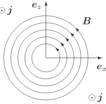
4.11.3 A Qubit in the Rotating Magnetic Field 177
4.11.4 Observing the Berry Phase Experimentally 183
5.1 Entangled States 191
5.2 Pauli Exclusion Principle 204
5.3 A Superconducting Biqubit 206
5.4 An Atom and a Photon 216
5.5 A Biqubit in a Rotated Frame 219
5.6 Bell Inequality 224
5.7 Nonlocality 230
5.8 Single-Qubit Expectation Values 233
5.9 Classification of Biqubit States 236
5.10 Separability 247
5.11 Impure Quantum Mechanics 259
5.11.1 Nonunitary Evolution 262
5.11.2 Depolarization 266
5.11.3 Dephasing 270
5.11.4 Spontaneous Emission 273
5.12 Schr¨odinger’s Cat 277
5.12.1 The Haroche-Ramsey Experiment 279
6
The Controlled
not
Gate
2896.1 The Quintessence of Quantum Computing 289
6.2 Universal Gates 292
6.2.1 TheABCDecomposition and Controlled-U 292
6.2.2 General Biqubit Unitary Gates 296
6.2.3 Triqubit Gates 303
6.2.4 Universality of the Deutsch Gate 306
6.3 The Cirac-Zoller Gate 322
7
Yes, It Can Be Done with Cogwheels
3437.1 The Deutsch Oracle 343
7.2 NMR Computing 352
7.3 Brassard Teleportation Circuit 362
7.4 The Grover Search Algorithm 371
7.5 Cogwheels 376
7.6 The Crossroad 387
A
Quaternions and Pauli Matrices
393A.1 Hamilton Quaternions 393
A.2 Pauli Quaternions 393
A.3 Pauli Matrices 395
B
Biqubit Probability Matrices
397C
Tensor Products of Pauli Matrices
399References 403
The Scientific and Engineering Series from MIT Press presents accessible accounts of computing research areas normally presented in research papers and specialized conferences. Elements of modern computing that have appeared thus far in the Series include parallelism, language design and implementation, systems software, and numerical libraries. The scope of the Series continues to expand with the spread of ideas from computing into new aspects of science.
One of the most revolutionary developments in computing is the discovery of algorithms for machines based not on operations on bits but on quantum states. These algorithms make possible efficient solutions to problems, such as factoring large numbers, currently thought to be intractable on conventional computers. But how do these machines work, and how might they be built?
This book presents in a down-to-earth way the concepts of quantum computing and describes a long-term plan to enlist the amazing—and almost unbelievable— concepts of quantum physics in the design and construction of a class of computer of unprecedented power. The engineering required to build such computers is in an early stage, but in this book the reader will find an engaging account of the necessary theory and the experiments that confirm the theory. Along the way the reader will be introduced to many of the most interesting results of modern physics.
This book arose from my occasional discussions on matters related to quantum computing with my students and, even more so, with some of my quite distinguished colleagues, who, having arrived at this juncture from various directions, would at times reveal an almost disarming lack of understanding of quantum physics fundamentals, while certainly possessing a formidable aptitude for skillfully juggling mathematics of quantum mechanics and therefore also of quantum computing— a dangerous combination. This lack of understanding sometimes led to perhaps unrealistic expectations and, on other occasions, even to research suggestions that were, well, unphysical.
Yet, as I discovered in due course, their occasionally pointed questions were very good questions indeed, and their occasional disbelief was well enough founded, and so, in looking for the right answers to them I was myself forced to revise my often canonical views on these matters.
From the perspective of a natural scientist, the most rewarding aspect of quantum computing is that it has reopened many of the issues that had been swept under the carpet and relegated to the dustbin of history back in the days when quantum mechanics had finally solidified and troublemakers such as Einstein, Schr¨odinger, and Bohm were told in no uncertain terms to “put up or shut up.” And so, the currently celebrated Einstein Podolsky Rosen paradox [38] lingered in the dustbin, not even mentioned in the Feynman’s Lectures on Physics [42] (which used to be my personal bible for years and years), until John Stewart Bell showed that it could be examined experimentally [7].
Look what the cat dragged in!
When Aspect measurements [4] eventually confirmed that quantum physics was indeed “nonlocal,” and not just on a microscopic scale, but over large macroscopic distances even, some called it the “greatest crisis in the history of modern physics.” Why should it be so? Newtonian theory of gravity is nonlocal, too, and we have been living with it happily since its conception in 1687. On the other hand, others spotted an opportunity in the crisis. “This looks like fun,” they said. “What can we do with it?” And this is how quantum computing was born. An avalanche of ideas and money that has since tumbled into physics laboratories has paid for many wonderful experiments and much insightful theoretical work.
this text were compared to texts covering classical computing, it would be a text about the most basic classical computing devices: diodes, transistors, gates. Such books are well known to people who are calledelectronic device engineers. Quantum Computing without Magicis a primer for futurequantum device engineers.
In classical digital computing everything, however complex or sophisticated, can be ultimately reduced to Boolean logic andnandor norgates. So, once we know
how to build anandor anorgate, all else is a matter of just connecting enough of
these gates to form such circuitry as is required. This, of course, is a simplification that omits power conditioning and managing issues, and mechanical issues—after all, disk drives rotate, have bearings and motors, as do cooling fans; and then we have keyboards, mice, displays, cameras, and so on. But the very heart of it all is Boolean logic and simple gates. Yet, the gates are no longer this simple when their functioning is scrutinized in more detail. One could write volumes about gates alone.
Quantum computing, on the other hand, has barely progressed beyond a single gate concept in practical terms. Although numerous learned papers exist that con-template large and nontrivial algorithms, the most advanced quantum computers of 2003 comprised mere two “qubits” and performed a single gate computation. And, as of early 2007, there hasn’t been much progress. Quantum computing is extremely hard to do. Why? This is one of the questions this book seeks to answer. Although Quantum Computing without Magicis a simple and basic text about qubits and quantum gates, it is not a “kindergarten” text. The readers are assumed to have mathematical skills befitting electronic engineers, chemists, and, certainly, mathematicians. The readers are also assumed to know enough basic quantum physics to not be surprised by concepts such as energy levels, Josephson junctions, and tunneling. After all, even entry-level students nowadays possess considerable reservoirs of common knowledge—if not always very detailed—about a great many things, including the world of quantum physics and enough mathematics to get by. On the other hand, the text attempts to explain everything in sufficient detail to avoid unnecessary magic—including detailed derivations of various formulas, that may appear tedious to a professional physicist but that should help a less experienced reader understand how they come about. In the spirit of stripping quantum computing of magic, we do not leave such results to exercises.
the density operator theory at this early stage, as well as a good understanding of what is actually being measured in quantum physics and how, can serve students well in their future careers.
Quantum mechanics is a probability theory. Although this fact is well known to physicists, it is often swept under the carpet or treated as somehow incidental. I have even heard it asked, “Where do quantum probabilities come from?”—as if this question could be answered by unitary manipulations similar to those invoked to explain decoherence. In the days of my youth a common opinion prevailed that quantum phenomena could not be described in terms of probabilities alone and that quantum mechanics itself could not be formulated in a way that would not require use of complex numbers. Like other lore surrounding quantum mechanics this opinion also proved untrue, although it did not become clear until 2000, when Stefan Weigert showed that every quantum system and its dynamics could be characterized fully in terms of nonredundant probabilities [145]. Even this important theoretical discovery was not paid much attention until Lucien Hardy showed a year later that quantum mechanics of discrete systems could be derived from “five reasonable axioms” all expressed in terms of pure theory of probability [60].
Why should it matter? Isn’t it just a question of semantics? I think it matters if one is to understand where the power of quantum mechanics as a theory derives from. It also matters in terms of expectations. Clearly, one cannot reasonably expect that a theory of probability can explain the source of probability, if such exists at all—which is by no means certain in quantum physics, where probabilities may be fundamental.
This book takes probability as a starting point. In Chapter 1 we discuss classical bits and classical registers. We look at how they are implemented in present-day computers. Then we look at randomly fluctuating classical registers and use this example to develop the basic formalism of probability theory. It is here that we introduce concepts of fiducial states, mixed and pure states, linear forms repre-senting measurements, combined systems, dimensionality, and degrees of freedom. Hardy’s theorem that combines the last two concepts is discussed as well, as it ex-presses most succinctly the difference between classical and quantum physics. This chapter also serves as a place where we introduce basic linear algebra, taking care to distinguish between vectors and forms, and introducing the concept of tensor product.
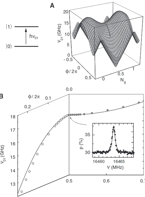
dif-ference between fully polarized and mixed states and demonstrate how an act of measurement breaks an initial pure state of the beam, converting it to a mixture. Eventually we arrive at the Bloch ball representation of qubit states. Then we introduce new concepts of Pauli vectors and forms. These will eventually map onto Pauli matrices two chapters later. But at this stage they will help us formulate laws of qubit dynamics in terms of pure probabilities—following Hardy, we call this simple calculus the fiducial formalism. It is valuable because it expresses qubit dynamics entirely in terms of directly measurable quantities. Here we discuss in detail Larmor precession, Rabi oscillations, and Ramsey fringes—these being fun-damental to the manipulation of qubits and quantum computing in general. We close this chapter with a detailed discussion of quantronium, a superconducting circuit presented in 2002 by Vion, Aassime, Cottet, Joyez, Pothier, Urbina, Esteve, and Devoret, that implemented and demonstrated the qubit [142].
Chapter 3 is short but pivotal to our exposition. Here we introduce quater-nions and demonstrate a simple and natural mapping between the qubit’s fiducial representation and quaternions. In this chapter we encounter the von Neumann equation, as well as the legendarytrace formula, which turns out to be the same as taking the arithmetic mean over the statistical ensemble of the qubit. We learn to manipulate quaternions by the means of commutation relations and discover the sole source of their power: they capture simultaneously in a single formula the cross and the dot products of two vectors. The quaternion formalism is, in a nutshell, the density operator theory. It appears here well before thewave function and follows naturally from the qubit’s probabilistic description.
Chapter 4 continues the story, beginning with a search for a simplest matrix representation of quaternions, which yields Pauli matrices. We then build the Hilbert space, which the quaternions, represented by Pauli matrices, act on and discover within it the images of the basis states of the qubit we saw in Chapter 2. We discover the notion of state superposition andderivethe probabilistic interpretation of transition amplitudes. We also look at the transformation properties of spinors, something that will come handy when we get to contemplate Bell inequalities in Chapter 5. We rephrase the properties of the density operator in the unitary language and then seek the unitary equivalent of the quaternion von Neumann equation, which is how we arrive at the Schr¨odinger equation. We study its general solution and revisit and reinterpret the phenomenon of Larmor precession. We investigate single qubit gates, a topic that leads to the discussion of Berry phase [12], which is further illustrated by the beautiful 1988 experiment of Richardson, Kilvington, Green, and Lamoreaux [119].
experimental examples. We strike while the iron is hot; otherwise who would believe such weirdness to be possible? We begin by showing a Josephson junction biqubit made by Berkley, Ramos, Gubrud, Strauch, Johnson, Anderson, Dragt, Lobb, and Wellstood in 2003 [11]. Then we show an even more sophisticated Josephson junc-tion biqubit made in 2006 by Steffen, Ansmann, Bialczak, Katz, Lucero, cDermott, Neeley, Weig, Cleland, and Martinis [134]. In case the reader is still not convinced by the functioning of these quantum microelectronic devices, we discuss a very clean example of entanglement between an ion and a photon that was demonstrated by Blinov, Moehring, Duan, and Monroe in 2004 [13]. Having (we hope) convinced the reader that an entangled biqubit is not the stuff of fairy tales, we discuss its representation in a rotated frame and arrive at Bell inequalities. We discuss their philosophical implications and possible ontological solutions to the puzzle at some length before investigating yet another feature of a biqubit—its single qubit expec-tation values, which are produced by partial traces. This topic is followed by a quite detailed classification of biqubit states, based on Englert and Metwally [39], and discussion of biqubit separability that is based on the Peres-Horodeckis criterion [113, 66].
Mathematics of biqubits is a natural place to discuss nonunitary evolution and to present simple models of important nonunitary phenomena such as depolarization, dephasing, and spontaneous emission. To a future quantum device engineer, these are of fundamental importance, inasmuch as every classical device engineer must have a firm grasp of thermodynamics. One cannot possibly design a working engine, or a working computer, while ignoring the fundamental issue of heat generation and dissipation. Similarly, one cannot possibly contemplate designing working quantum devices while ignoring the inevitable loss of unitarity in every realistic quantum process.
We close this chapter with the discussion of the Schr¨odinger cat paradox and a beautiful 1996 experiment of Brune, Hagley, Dreyer, Maitre, Maali, Wunderlich, Raimond, and Haroche [18]. This experiment clarifies the muddled notion of what constitutes a quantum measurement and, at the same time, is strikingly “quantum computational” in its concepts and methodology.
The last major chapter of the book, Chapter 6. puts together all the physics and mathematics developed in the previous chapters to strike at the heart of quantum computing: the controlled-notgate. We discuss here the notion of quantum gate
universality and demonstrate, following Deutsch [29], Khaneja and Glaser [78], and Vidal and Dawson [140], that the controlled-not gate is universal for quantum
elegant 2003 implementation by Schmidt-Kaler, H¨affner, Riebe, Gulde, Lancaster, Deuschle, Bechner, Roos, Eschner, and Blatt [125]. On this occasion we also discuss the functioning of the linear Paul trap, electron shelving technique, laser cooling, and side-band transitions, which are all crucial in this experiment. We also look at the 2007 superconducting controlled-notgate developed by Plantenberg, de Groot,
Harmans, and Mooij [114] and at the 2003 all-optical controlled-notgate
demon-strated by O’Brien, Pryde, White, Ralph, and Branning [101].
In the closing chapter of the book we outline a roadmap for readers who wish to learn more about quantum computing and, more generally, about quantum infor-mation theory. Various quantum computing algorithms as well as error correction procedures are discussed in numerous texts that have been published as far back as 2000, many of them “classic.” The device physics background provided by this book should be sufficient to let its readers follow the subject and even read professional publications in technical journals.
But there is another aspect of the story we draw the reader’s attention to in this chapter. How “quantum” is quantum computing? Is “quantum” really so unique and different that it cannot be faked at all by classical systems? When compar-isons are made between quantum and classical algorithms and statements are made along the lines that “no classical algorithm can possibly do this,” the authors, rather narrow-mindedly, restrict themselves to comparisons with classical digital algorithms. But the principle of superposition, which makes it possible for quan-tum algorithms to attain exponential speedup, is not limited to quanquan-tum physics only. The famous Grover search algorithm can be implemented on a classical analog computer, as Grover himself demonstrated together with Sengupta in 2002 [57]. It turns out that a great many features of quantum computers can be implemented by using classical analog systems, even entanglement [24, 133, 103, 104, 105]. For a device engineer this is a profound revelation. Classical analog systems are far easier to construct and operate than are quantum systems. If similar computa-tional efficiencies can be attained this way, may not this be an equally profitable endeavor? We don’t know the full answer to this question, perhaps because it has not been pursued with as much vigor as has quantum computing itself. But it is an interesting fundamental question in its own right, even from a natural scientist’s point of view.
state is needed, the whole statistical ensemble that represents the state must be explored. After all, what is a “quantum state” if not an abstraction that refers to the vector of probabilities that characterize it [60]? And there is but one way to arrive at this characterization. One has to measure and record sometimes hundreds of thousands of detections in order to estimate the probabilities with such error as the context requires.
And don’t you ever forget it!
This, of course, does have some bearing on the cost and efficiency of quantum computation, even if we were to overlook quantum computation’s energetic ineffi-ciency [49], need for extraordinary cooling and isolation techniques, great complex-ity and slowness of multiqubit gates, and numerous other problems that all derive from . . .physics. This is where quantum computing gets stripped of its magic and dressed in the cloak of reality. But this is not a drab cloak. It has all the coarseness and rich texture of wholemeal bread, and wholemeal bread is good for you.
Acknowledgments
This book owes its existence to many people who contributed to it in various ways, often unknowingly, over the years. But in the first place I would like to thank the editors for their forbearance and encouragement, and to Gail Pieper, who patiently read the whole text herself and through unquestionable magic of her craft made it readable for others.
To Mike McRobbie of Indiana University I owe the very idea that a book could be made of my early lecture notes, and the means and opportunity to do so. Eventually, little of my early notes made it into the book, which is perhaps for the better.
I owe much inspiration, insights and help to my professional colleagues, Zhenghan Wang, Lucien Hardy, Steven Girvin, and Mohammad Amin, whose comments, sug-gestions, ideas, and questions helped me steer this text into what it has eventually become.
My interest in the foundations of quantum mechanics was awoken many years ago by Asher Peres, who visited my alma mater briefly and talked about the field, and by two of my professors Bogdan Mielnik and Iwo Birula-Bialynicki. Although I understood little of it at the time, I learned that the matter was profound and by no means fully resolved. It was also immensely interesting.
sense that, ultimately, helped me navigate through the murky waters of quantum computing and quantum device engineering.
“If you want to amount to anything as a witch, Magrat Garlick, you got to learn three things. What’s real, what’s not real, and what’s the difference—”
1.1
Physical Embodiments of a Bit
Information technology devices, such as desktop computers, laptops, palmtops, Bits and bytes cellular phones, and DVD players, have pervaded our everyday life to such extent
that it is difficult to find a person who would not have at least some idea about what bits and bytes are. I shall assume therefore that the reader knows about both, enough to understand that a bit is the “smallest indivisible chunk of information” and that a byte is a string of eight bits.
Yet the concept of a bit as the smallest indivisible chunk of information is a Discretization of information is a convention. somewhat stifling convention. It is possible to dose information in any quantity,
not necessarily in discrete chunks, and this is how many analog devices, including analog computers, work. What’s more, it takes a considerable amount of signal processing, and consequently also power and time, to maintain a nice rectangular shape of pulses representing bits in digital circuits. Electronic circuits that can handle information directly, without chopping it to bits and arranging it into bytes, can be orders of magnitude faster and more energy efficient than digital circuits.
How are bits and bytes actually stored, moved, and processed inside digital de- Storing and manipulating bits
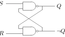
vices? There are many ways to do so. Figure 1.1 shows a logic diagram of one of the simplest memory cells, a flip-flop.
The flip-flop in Figure 1.1 comprises two cross-couplednandgates. It is easy to A flip-flop as a
1-bit memory cell
analyze the behavior of the circuit. Let us supposeR is set to 0 andS is set to 1. IfRis 0, then regardless of what the second input to thenandgate at the bottom
is, its output must be 1. Therefore the second input to thenandgate at the top is
1, and so its output Qmust be 0. The fact that the roles ofRandS in the device are completely symmetric implies that if R is set to 1 and S to 0, we’ll get that
Q= 1 and ¬Q= 0. Table 1.1 sums up these simple results.
R S
¬Q Q
Table 1.1: Qand¬Qas functions ofRand S for the flip-flop of Figure 1.1.
R S Q ¬Q
0 1 0 1
1 0 1 0
2 kΩ 2 kΩ
❘ A
B
+5 V
¬(A∧B)
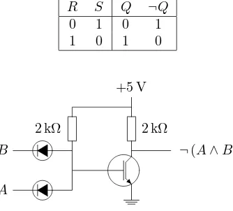
Figure 1.2: A diode-transistor-logic implementation of anandgate.
We observe that once the value ofQ has been set to either 0 or 1, setting both
R andS to 1 retains the preset value ofQ. This is easy to see. Let us supposeQ
has been set to 1. Therefore¬Qis 0, and so one of the inputs to the uppernand
gate is 0, which implies that its output must be 1. In order for ¬Qto be 0, both inputs to the lowernandgate must be 1, and so they are, becauseR= 1.
Now suppose thatQhas been preset to 0 instead. In this case the second input to the lowernandgate is 0, and therefore the output of the gate,¬Qis 1, which is
exactly what is required in order forQto be 1, on account of¬Qbeing the second input to the uppernandgate.
And so our flip-flop behaves like a simple memory device. By operating on its inputs we can set its output to either 0 or 1, and then by setting both inputs to 1 we can make it remember the preset state.
It is instructive to have a closer look at what happens inside thenandgates when
What is inside
thenand gate the device remembers its preset state. How is this remembering accomplished?
Figure 1.2 shows a simple diode-transistor logic (DTL) implementation of anand
Table 1.2: Truth table of the DTLnandgate shown in Figure 1.2.
A B ¬(A∧B)
0 0 1
0 1 1
1 0 1
1 1 0
either of the two inputs is set to 0. In this case the corresponding diode conducts, and the positive charge drains from the gate of the transistor. Consequently its channel blocks and the output of the circuit ends up being 1. On the other hand, if both inputs are set to 1, both diodes block. In this case positive charge flows toward the gate of the transistor and accumulates there, and the transistor channel conducts. This sets the potential on the output line to 0. The resulting truth table of the device is shown in Table 1.2. This is indeed the table of anandgate.
The important point to observe in the context of our considerations is that it is the presence or the absence of the charge on the transistor gate that determines the value of the output line. If there is no accumulation of positive charge on the gate, the output line is set to 0; if there is a sufficient positive charge on the gate, the output line is set to 1.
Returning to our flip-flop example, we can now see that the physical embodiment The gate charge embodies the bit. of the bit, which the flip-flop “remembers,” is the electric charge stored on the gate
of the transistor located in the uppernand gate of the flip-flop circuit. If there
is an accumulation of positive charge on the transistor’s gate, the Q line of the flip-flop becomes 0; and if the charge has drained from the gate, theQline becomes 1. TheQline itself merely provides us with the means of reading the bit.
We could replace the flip-flop simply with a box and a pebble. An empty box would correspond to a drained transistor gate, and this we would thenread as 1. If we found a pebble in the box, we would read this as 0. The box and the pebble would work very much like the flip-flop in this context.
It is convenient to reverse the convention and read a pebble in the box as 1 and A pebble in a box
its absence as 0. We could do the same, of course, with the flip-flop, simply by renamingQto¬Qand vice versa.
Seemingly we have performed an act of conceptual digitization in discussing and then translating the physics of the flip-flop and of the DTLnandgate to the box
A transistor is really an analog amplifier, and one can apply any potential to its gate, which yields a range of continuous values to its channel’s resistance. In order for the transistor to behave like a switch and for the circuit presented in Figure Continuous
transitions between states
1.2 to behave like a nandgate, we must condition its input and output voltages:
these are usually restricted to {0 V,+5 V} and switched very rapidly between the two values. Additionally, parts of the circuit may be biased at −5 V in order to provide adequate polarization. Even then, when looked at with an oscilloscope, pulses representing bits do not have sharp edges. Rather, there are transients, and these must be analyzed rigorously at the circuit design stage in order to eliminate unexpected faulty behavior.
On the other hand, the presence or the absence of the pebble in the box appar-ently represents two distinct, separate states. There are no transients here. The pebble either is or is not in the box. Tertium non datur.
Yet, let us observe that even this is a convention, because, for example, we could place the pebble in such a way that only a half of it would be in the box and the other half would be outside. How should we account for this situation?
In binary, digital logic we ignore such states. But other types of logic do allow Many-valued
logic for the pebble to be halfway or a third of the way or any other portion in the box. Such logic systems fall under the category of many-valued logics [44], some of which are even infinitely valued. An example of an infinitely valued logic is the popular fuzzy logic [81] commonly used in robotics, data bases, image processing, and expert systems.
When we look at quantum logic more closely, these considerations will acquire a new deeper meaning, which will eventually lead to the notion of superposition of quantum states. Quantum logic is one of these systems, where a pebble can be halfway in one box and halfway in another one.
And the boxes don’t even have to be adjacent.
1.2
Registers
A row of flip-flops connected with each other in various ways constitutes a register. A 3-bit counter
Depending on how the flip-flops are connected, the register may be used just as a store, or it can be used to perform some arithmetic operations.
Figure 1.3 shows a simple 3-bit modulo-7 counter implemented with threeJK
J Q J Q J Q
K Q¯ K Q¯ K Q¯
T T T
ABC
clock
clear
Figure 1.3: A modulo-7 counter made of threeJK flip-flops.
1. The stateQof theJK flip-flop toggles on thetrailing edge of the clock pulse
T, that is, when the state of the inputT changes from 1 to 0; 2. Applying 0 toclearresetsQto 0.
Let us assume that the whole counter starts in the {C = 0, B = 0, A = 0}
state. On the first application of the pulse to the clock input, A toggles to 1 on Register states the trailing edge of the pulse and stays there. The state of the register becomes
{C= 0, B= 0, A= 1}. On the second application of the clock pulseAtoggles back to 0, but this change now toggles B to 1, and so the state of the register becomes {C = 0, B = 1, A= 0}. On the next trailing edge of the clock pulse A toggles to 1 and the state of the register is now {C = 0, B = 1, A = 1}. When A toggles back to 0 on the next application of the clock pulse, this triggers the change inB
from 1 to 0, but this in turn toggles C, and so the state of the register becomes {C= 1, B= 0, A= 0}, and so on. DroppingC=,B=, andA= from our notation describing the state of the register, we can see the following progression:
{000} → {001} → {010} → {011} → {100} →. . . . (1.1) We can interpret the strings enclosed in curly brackets as binary numbers; and upon having converted them to decimal notation, we obtain
0→1→2→3→4→. . . . (1.2)
become 1 at the same time, thenandgate at the bottom of the circuit appliesclear
to all three flip-flops, and soA, B, andC get reset to 0. This process happens so fast that the counter does not stay in the {111} configuration for an appreciable amount of time. It counts from 0 through 6 transitioning through seven distinct stablestates in the process.
At first glance we may think that the counterjumpsbetween the discrete states. State transitions
A closer observation of the transitions with an oscilloscope shows that the counter glidesbetween the states through a continuum of various configurations, which can-not be interpreted in terms of digital logic. But the configurations in the continuum are unstable, and the gliding takes very little time, so that the notion ofjumps is a good approximation.1
By now we know that a possible physical embodiment of a bit is an accumulation of electric charge on the gate of a transistor inside a flip-flop. We can also think about the presence or the absence of the charge on the gate in the same way we think about the presence or absence of a pebble in a box. And so, instead of working with a row of flip-flops, we can work with a row of boxes and pebbles. Such a system is also a register, albeit a much slower one and more difficult to manipulate.
The following figure shows an example of a box and a pebble register that displays An “almost
quantum” register
some features that are reminiscent of quantum physics.
The register contains three boxes stacked vertically. Their position corresponds to the energy of a pebble that may be placed in a box. The higher the location of the box, the higher the energy of the pebble. The pebbles that are used in the register have a peculiar property. When two pebbles meet in a single box, they annihilate, and the energy released in the process creates a higher energy pebble in the box above. Of course, if there is already a pebble there, the newly created pebble and the previously inserted pebble annihilate, too, and an even higher energy pebble is created in the next box up.
1An alert reader will perhaps notice that what we call ajump in our everyday life is also a
the bottom of the stack. When we place the first pebble there, the system looks as follows.
•
Now we add another pebble to the box at the bottom. The two pebbles annihilate, and a new, higher-energy pebble is created in the middle box.
••
→bang! → •
When we add a pebble again to the box at the bottom, nothing much happens, because there is no other pebble in it, and so the state of the register becomes as shown below.
• •
But fireworks fly again when we add a yet another pebble to the box at the bottom of the stack.
••
• →bang! → •• →bang! →
•
box. But a pebble is already there, so the two annihilate in the second bang, and a pebble of even higher energy is now created in the top box.
In summary, the register has transitioned through the following stable states:
→ •
→ • → • • →
•
The register, apparently, is also a counter. Eventually we’ll end up having pebbles in all three boxes. Adding a yet another pebble to the box at the bottom triggers a chain reaction that will clear all boxes and will eject a very high energy pebble from the register altogether. This, therefore, is a modulo-7 counter.
The first reason the register is reminiscent of a quantum system is that its succes-Creation and
annihilation operators
sive states are truly separate, without any in-betweens; that is, pebbles don’t move between boxes. Instead they disappear from a box; and if the energy released in the process is high enough, a new pebble reappears from nothingness in a higher-energy box. The model bears some resemblance to quantum field theory, where particle states can be acted on by annihilation and creation operators. We shall see similar formalism applied in the discussion of vibrational states in the Paul trap in Section 6.3, Chapter 6.
The second reason is that here we have a feature that resembles the Pauli ex-clusion principle, discussed in Section 5.2, Chapter 5, which states that no two fermions can coexist in the same state.
1.3
Fluctuating Registers
The stable states of the register we have seen in the previous sections were all well defined. For example, the counter would go through the sequence of seven stable configurations:
register set by some electronic procedure to hold a binary number {101}—there may be
some toggle switches to do this on the side of the package—its bits start to fluctuate randomly so that the register spends only 72% of the time in the{101}configuration and 28% of the time in every other configuration, flickering at random between them3.
Let us assume that the same happens when the register is set to hold other numbers, {000},{001}, . . . ,{111} as well; that is, the register ends up flickering between all possible configurations at random but visits itsset configuration 72% of the time. At first glance a register like this seems rather useless, but we could employ its fluctuations, for example, in Monte Carlo codes.
To make the game more fun, after the register has been set, we are going to cover its toggles with a masking tape, so that its state cannot be ascertained by looking at the toggles. Instead we have to resort to other means. The point of this exercise is to prepare the reader for a description of similar systems that have no toggles at all.
The register exists in one of the eight fluctuating states. Each state manifests Flactuating register states itself by visiting a certain configuration more often than other configurations. This
time we can no longer associate the state with a specific configuration as closely as we have done for the register that was not subject to random fluctuations. The state is now something more abstract, something that we can no longer associate with a simple single observation of the register. Instead we have to look at the register for a long time in order to identify its preferred configuration, and thus its state.
Let us introduce the following notation for the states of the fluctuating register:
p¯0 is the state that visits{000}most often, p¯1 is the state that visits{001}most often, p¯2 is the state that visits{010}most often, p¯3 is the state that visits{011}most often, p¯4 is the state that visits{100}most often, p¯5 is the state that visits{101}most often,
p¯6 is the state that visits{110}most often,
p¯7 is the state that visits{111}most often.
Although we have labeled the statesp¯0 throughp¯7, we cannot at this early stage associate the labels with mathematical objects. To endow the states of the fluctu-ating register with a mathematical structure, we have to figure out how they can be measured and manipulated—and then map this onto mathematics.
So, how can we ascertain which one of the eight states defined above the register State
observation is in, if we are not allowed to peek at the setting of its switches?
To do so, we must observe the register for a long time, writing down its observed configurations perhaps at random time intervals.4 If the register is in thep¯
5state,
approximately 72% of the observations should return the{101}configuration, with other observations evenly spread over other configurations. If we maden5 measure-ments of the register in total,n0
5observations would show the register in the{000}
configuration, n15 observations would show it in the {001} configuration, and so
on for every other configuration, ending withn7
5for the{111}configuration.5 We
can now build a column vector for which we would expect the following:
⎛
We do not expectn65/n5= 0.04 exactly, because, after all, the fluctuations of the
register are random, but we do expect that we should get very close to 0.04 ifn5is very large. Forn5→ ∞the ratios in the column vector above becomeprobabilities. This lets us identify statep¯5with the column of probabilities of finding the register
State description
4An important assumption here is that we can observe the register without affecting its state,
which is the case with classical registers but not with quantum ones. One of the ways to deal with it in the quantum case is to discard the observed register and get a new one in the same state for the next observation. Another way is to reset the observed register, if possible, put it in the same state, and repeat the observation.
5The superscripts 0 through 7 inn0
5 throughn75 and also inp05 throughp75 further down
arenotexponents. We do not raisen5(orp5) to the powers of 0 through 7. They are just indexes,
which say that, for example,n4
5 is the number of observations made on a register in statep¯5
that found it in configuration{100} ≡4. There is a reason we want this index to be placed in the superscript position rather than in the subscript position. This will be explained in more detail when we talk about forms and vectors in Section 1.7 on page 28. If we ever need to exponentiate an object with a superscript index, for example,p3
5, we shall enclose this object in brackets to
distinguish between a raised index and an exponent, for example,`
p¯5≡
It is often convenient to think of the fluctuating register in terms of astatistical A statistical ensemble of registers ensemble.
Let us assume that instead of a single fluctuating register we have a very large number of static, nonfluctuating registers, of which 4% are in the{000} configura-tion, 4% are in the {001}configuration, 4% are in the{010}configuration, 4% are in the{011}configuration, 4% are in the{100}configuration, 72% are in the{101} configuration, 4% are in the{110}configuration, and 4% are in the{111} configu-ration. Now let us put all the registers in a hat, mix them thoroughly, and draw at randomn5 registers from the hat. Of thesen0
5 will be in the{000} configuration, n1
5 in the{001} configuration,. . .,n65 in the{110} configuration andn75 in the
{111} configuration. If the wholeensemble has been mixed well, we would expect the following:
Logically and arithmetically such an ensemble of static registers from which we sample n5registers is equivalent to a single randomly fluctuating register at which welook (without disturbing its overall condition)n5 times.
the following column vectors of probabilities:
We shall call the probabilities that populate the arraysfiducial measurements, and we shall call the arrays of probabilitiesfiducial vectors6 [60].
For every statep¯i,i= 0,1, . . . ,7, listed above, we have thatp0
i+p1i+p2i+p3i+
p4
i+p5i+p6i+p7i= 1. This means that the probability of finding the register in
any one of the configurations from{000} through{111} is 1. Statesp¯i that have this property are said to benormalized.
Given the collection of normalized statesp¯iwe can construct statistical ensembles with other values for probabilities p0 through p7 by mixing states p¯
i in various
proportions.
6The wordfiducialin physics means an object or a system that is used as a standard of reference
Let us suppose we have a very large number,N, of fluctuating registers affected by the malady discussed in the previous section. Let us also suppose thatN0of these have been put in state p¯0 and the remainingN−N0=N3 have been put in state
p¯3.
Now let us place all N registers into a hat and mix them thoroughly. We can Mixing statistical ensembles draw them from the hat at random and look at their configuration but only once
per register drawn. What probabilities should we expect for any possible register configuration in the ensemble?
The easiest way to answer the question is toexpand statesp¯0 andp¯3 into their
corresponding statistical ensembles and say that we have N0 ensembles that cor-respond to state p¯0 and N3 ensembles that correspond to state p¯3. In each p¯0
ensemble we have n0
0 registers out of n0 in the {000} configuration, and in each p¯3 ensemble we haven03 registers out ofn3 in the{000}configuration. Hence, the
total number of registers in the{000}configuration is
N0n0
0+N3n03. (1.6)
The total number of registers after this expansion of states into ensembles is
N0n0+N3n3. (1.7)
Therefore, the probability of drawing a register in the{000}configuration is going to be
N0n0
0+N3n03
N0n0+N3n3 , (1.8)
in the limitN → ∞,n0→ ∞, andn3→ ∞.
We should also assume at this stage that we have an identical number of registers in the ensembles forp¯0 andp¯3, that is, thatn0=n3=n. The reason is that if the
ensembles for p¯0have, say, a markedly smaller number of registers than ensembles forp¯0, the latter will weigh more heavily than the former, and so our estimates of
probabilities for the whole mixture, based on finite sampling, will be skewed. Then
N0n0
0+N3n03 N0n0+N3n3
=N0n
0
0+N3n03 n(N0+N3) =
N0n0
0+N3n03
nN =
N0 N
n0 0 n +
N3 N
n0 3 n .
In the limitn→ ∞andN → ∞this becomes
where P0 is the probability of drawing a register in statep¯0, P3 is the probability of drawing a register in statep¯3,p00is the probability that a register in statep¯0is
observed in configuration{000}, and p0
3 is the probability that a register in state p¯3 is observed in configuration{000}.
To get a clearer picture, let us assume thatP0= 0.3 and thatP3= 0.7. At this level (of probabilities pertaining to the mixture) we have thatP0+P3= 1. What are the probabilities for each configuration in the mixture?
p0=P0p00+P3p03 = 0.3·0.72 + 0.7·0.04 = 0.244, p1=P0p10+P3p13 = 0.3·0.04 + 0.7·0.04 = 0.04, p2=P0p20+P3p23 = 0.3·0.04 + 0.7·0.04 = 0.04, p3=P0p30+P3p33 = 0.3·0.04 + 0.7·0.72 = 0.516, p4=P0p40+P3p43 = 0.3·0.04 + 0.7·0.04 = 0.04, p5=P0p50+P3p53 = 0.3·0.04 + 0.7·0.04 = 0.04, p6=P0p60+P3p63 = 0.3·0.04 + 0.7·0.04 = 0.04, p7=P0p70+P3p73 = 0.3·0.04 + 0.7·0.04 = 0.04.
The mixture remains normalized. All probabilitiespi,i= 1, . . . ,7, still add to one.
Using symbol p for the array of probabilities p0 through p7, we can write the
Fiducial vector
above as follows:
p=P0p¯0+P3p¯3. (1.10)
In general, assuming that we use all possible states in the mixture, we would have
p=
i
Pip¯i. (1.11)
The mixture state is a linear combination of its constituents. The linearity is restricted by two conditions, namely, that iPi= 1 and∀i0≤Pi ≤1. Linearity
Convexity
so restricted is calledconvexity, but we are going to show in Section 1.6 that it can be extended to full linearity as long as what is on the left-hand side of equation (1.11) is still a physically meaningful state.
One can easily see that kpk = 1 for any convex linear combination that
repre-sents a mixture
k
pk =
k
i
Pipki=
i
Pi
k
pk i=
=
i
Pi·1 =
i
by the array
can be thought of as a mixture of, say, 1,000,000 nonfluctuating registers, of which 720,000 are in the {011}configuration at all times and the remaining 280,000 reg-isters are evenly spread over the remaining configurations, with 40,000 regreg-isters in each.
A register that is in a nonfluctuating {000} configuration can still be described Pure states in terms of a column vector of probabilities as follows:
⎛
One can easily see why this should be so. For 0 < pi < 1 we have that 0 <
Let us introduce the following notation for the pure states: Fiducial
This time we have dropped the bars above the digits to emphasize that thesepure states do not fluctuate and therefore the digits that represent them are exact and do not represent averages or most often encountered configurations.
Let us consider a randomly fluctuating register state specified by a vector of The basis of
pure states probabilitiesp. Using straightforward array arithmetic, we can express the array
pin terms ofei as follows:
p=
i
piei. (1.17)
The expression is reminiscent of equation (1.11) on page 14, but here we have replaced fluctuating states on the right-hand side with nonfluctuatingpure states. And so, we have arrived at the following conclusion:
Every randomly fluctuating register state is a mixture of pure states.
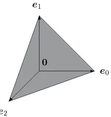
The ability to decompose any randomly fluctuating register statepinto a linear Vector space
✲ e0 ✻
✠ e2
0
Figure 1.4: The setS in the three-dimensional vector space that corresponds to a 2-bit modulo-3 fluctuating register is the gray triangle spanned by the ends of the three basis vectors of the space.
the natural choice for the basis are the pure states.7 But fluctuating states do not
fill the space entirely, because only vectors for which
i
pi= 1 and ∀i0≤pi≤1, (1.18)
are physical. Let us call the set of physically meaningful vectors in this space S.
Figure 1.4 shows set S for a three-dimensional vector space that corresponds A set of physically meaningful states to a 2-bit modulo-3 fluctuating register, that is, a register, for which the {11} configuration is unstable and flips the register back to {00}.
In this case S is the triangle spanned by the tips of the pure states.
e0≡ ⎛
⎝
1 0 0
⎞
⎠, e1≡ ⎛
⎝
0 1 0
⎞
⎠, e2≡ ⎛
⎝
0 0 1
⎞
⎠. (1.19)
One can fill the space between the triangle in Figure 1.4 and the zero of the The null state vector space by admitting thenull state as a possible participant in the mixtures.
7We are going toload the termbasiswith an additional meaning soon, but what we have just
A 3-bit register null state, for which we are going to use symbol0, corresponds to the array of probabilities
0≡
The meaning of the null state is that a register in this state does not return any acceptable reading at all: we can say that it’s broken, that all its LEDs are off.
Let us consider the following mixture: 30% of the 3-bit registers are in the null state 0, 40% of the 3-bit registers are in the e2 state, and the remaining 30% are in the e4 state. What are the coefficients pi of the mixture? Let us expand
the mixture into its statistical ensemble, assuming for simplicity that the total number of registers in the ensemble is 100. Then 40 registers will be in the {010} configuration, 30 registers will be in the{100}configuration, and the remaining 30 registers will be in no readable configuration at all. The probability of drawing a register in the{010}configuration from the ensemble is thereforep2= 40/100 =.4.
The probability of drawing a register in the{100}configuration from the ensemble isp4= 30/100 =.3. The probability of drawing a register in any other acceptable
configuration is 0. The resulting state of the register is therefore as follows:
p≡
A state vector for which ipi <1 is said to beunnormalized as opposed to a
Diluted mixtures
state vector for which ipi = 1, which, as we have already remarked, is said to
not diluted either: these states are normalized, and they are also mixtures. If null states are allowed, then the corresponding setS is no longer restricted to the surface of the triangle shown in Figure 1.4. Instead, the states fill the whole volume of the tetrahedron between the triangle and the zero of the vector space, including both the zero and the triangle.
The pure states and the null state are theextremalpoints ofS. This observation Pure states as extremal points of S
lets us arrive at the followingdefinition of pure states:
Pure states correspond to extremal points ofS− {0}.
The definition will come handy in more complex situations and in richer theories, in which we may not be able to draw a simple picture or recognize that a given state is pure by merely looking at its corresponding column of probabilities.
1.5
Basis States
In Section 1.4 we stated that pure states were the natural choice for the basis of the vector space in which physical states of fluctuating registers filled set S. This assertion was based on elementary algebra, which we used to decompose an arbitrary mixture into a linear combination of pure states,
p=
7
i=0
piei. (1.22)
The decomposition, in turn, was based on the representation of pure states by arrays of zeros and ones—arrays, which in the world of elementary algebra are commonly associated with basis vectors.
Here we are going to give a quite special physical meaning to what we are going A basis state to call thebasis state throughout the remainder of this book and to what is also
called the basis state in quantum mechanics.
Abasis stateis the configuration of a randomly fluctuating register that can be ascertained by glancing at it momentarily.
If we have a fluctuating register and “glance at it momentarily,” we are not going to Physical and canonical basis states
see it fluctuate. Instead, we are going to see this register in a quite specific frozen (albeit momentarily only) configuration, for example,{010}. If we glance at the register again a moment later, the register may be in the{101}configuration.8 We
are going to call the nonfluctuating states that correspond to these configurations (such ase2ande5) the physical basis states. Altogether we are going to have eight such basis states for the classical 3-bit randomly fluctuating register, assuming that all bits are allowed to fluctuate freely. The basis states, as defined here, are e0
through e7, which is also what we have called “pure states” and what is also a canonical basis in the fiducial vector space.
We are going to use a special notation for such momentarily glanced basis vectors to distinguish between them and the canonical basis. Borrowing from the traditions of quantum mechanics, we’ll denote them by|e0 through|e7 .
The number of vectors in the physical basis of the classical randomly fluctuat-Dimensionality
and degrees of freedom
ing register—this number is also called the dimensionality of the system—is the same as the number of probabilities needed to describe the state. The number of probabilities is also called the number of degrees of freedom of the system. This follows clearly from how the probabilities have been defined: they are probabilities of finding the register in one of its specific configurations, which here we have iden-tified with the basis states, because these are the only configurations (and not the fluctuating states) that we can actually see when we give the register a brief glance. Denoting the dimensionality of the system by N and the numbers of degrees of freedom byK, we can state that for the classical randomly fluctuating register
K=N. (1.23)
Why should we distinguish at all between canonical and physical basis, especially since they appear to be exactly the same for the case considered so far? The answer is that they will not be the same in the quantum register case. What’s more, we shall find there that
K=N2. (1.24)
A perspicacious reader may be tempted to ask the following question: What if I Transitional
configurations happen to catch the register in one of theunstable states it goes through when it glidesbetween the configurations described by symbols{000}through{111}? Such a configuration does not correspond to any of the “basis vectors” we have defined in this section.
This is indeed the case. Our probabilistic description does not cover the configu-rations of the continuum through which the register glides between itsbasis states at all. Instead we have focused entirely on the stable discrete configurations.
One of the ways to deal with the problem is to define more precisely what we mean The meaning of
switch during observation. If the register stays in any given configuration for Δt
on average, then we want “momentarily” to be much shorter than Δt. And so we arrive at a somewhat more precise definition of “momentarily”:
δt≪“momentarily”≪Δt. (1.25)
We shall see that this problem is not limited to classical registers. A similar condition is imposed on quantum observations, although the dynamics of quantum observations is quite different. But it still takes a certain amount of time and effort to force a quantum system into its basis state. If the act of observation is too lightweight and too fast, the quantum system will not “collapse” to the basis state, and the measurement will end up being insufficiently resolved.
A quite different way to deal with the problem is to include the continuum of Inclusion of transitional states configurations the register glides through between its stable states into the model and to allow register configurations such as{0.76 0.34 0.18}. We would then have to add probabilities (or probability densities) of finding the register in such a state to our measurements and our theory. The number of dimensions of the system would skyrocket, but this does not necessarily imply that the system would become intractable.
This solution also has its equivalent in the world of quantum physics. Detailed investigations of the spectrum of hydrogen atom revealed that its spectral lines were split into very fine structure and that additional splitting occurred in presence of electric and magnetic fields. To account for every observed feature of the spectrum, physicists had to significantly enlarge the initially simple theory of hydrogen atom so as to incorporate various quantum electrodynamic corrections.
1.6
Functions and Measurements on Mixtures
How can we define a function on a randomly fluctuating registerstate?
There are various ways to do so. For example, we could associate certain values,
fi ∈ R, with specific configurations of the register, that is,{000}, . . . ,{111}, and
then we could associate an average of fi over the statistical ensemble that
corre-sponds topwithf(p). This is a very physical way of doing things, since all that we Averages can see as we glance at the fluctuating register every now and then are its various
basis states, its momentarily frozen configurations. If every one of the configura-tions is associated with some valuefi, what we’re going to perceive in terms offi
over a longer time, as the register keeps fluctuating, is an average value offi.
construct an arbitrary mapping of the form
S ∋p→f
p0, p1, p2, p3, p4, p5, p6, p7
∈R, (1.26)
whereRstands for real numbers.
The second way is very general and could be used to define quite complicated nonlinear functions on coefficientspi, for example,
S∋p→
p02
+p1p3−sin
p2p3p4
+ep5p6p7 ∈R. (1.27) A function like this could be implemented by an electronic procedure. For example, the procedure could observe the register for some time collecting statistics and building a fiducial vector for it. Once the vector is sufficiently well defined, the above operation would be performed on its content and the value off delivered on output. Knowing value offon the basis states would not in general help us evaluate
f on an arbitrary state p. Similarly, knowing values off on the components of a mixture would not in general help us evaluatef on the mixture itself. In every case we would have to carry out full fiducial measurements for the whole mixture first, and only evaluate the function afterward.
On the other hand, the strategy outlined at the beginning of the section leads to functions that can be evaluated on the go and have rather nice and simple properties. Also, they cover an important special case: that of the fiducial vector itself.
Let us consider a register that has a tiny tunable laser linked to its circuitry and the coupling between the laser and the configuration of the register is such that when the register is in configuration{000}, the laser emits red light; when the register is in configuration{111}, the laser emits blue light; and when the register is in any of the intermediate configurations, the laser emits light of some color between red and blue. Let the frequency of light emitted by the laser when the register is in stateei(which corresponds directly to a specific configuration) befi.
Let us then define the frequency functionf on the basis states9as
f(ei)=. fi. (1.28)
We are going to extend the definition to an arbitrary mixture p = ipie i by
calculating the average value of fi over the ensemble that corresponds top. Let
us call the average value ¯f and let us use the arithmetic mean formula to calculate Arithmetic
mean over the
ensemble 9These are, in fact, physical basis states, because we want to associate the definition with
register configurations that can be observed by glancing at the register momentarily. So we should really write here|ei. But let us recall that for the classical register they are really the
registers are in statee1,. . ., andnp7registers are in statee7. The arithmetic mean
of fi over the ensemble is
¯
Now let us take two arbitrary states10
p1=
and evaluatef on their mixture:
f(P1p1+P2p2) = f
We find thatf isconvex on mixtures, or, in other words, it is linear on expressions Convexity of arithmetic mean of the formP1p1+P2p2, wherep1andp2belong toS, 0≤P1≤1 and 0≤P2≤1
and P1+P2= 1.
10These are no longer the same states as our previously defined states p ¯
1 and p¯2: the bars
We can extend the definition of f to diluted mixtures by adding the following condition:
f(0) = 0. (1.33)
Returning to our model where fi is a frequency of light emitted by a tunable
laser linked to a register configuration that corresponds to state ei, f(p) is the
combined color of light emitted by the laser as the register in state p fluctuates randomly through various configurations. The color may be different from all col-ors of frequencies fi that are observed by glancing at the register momentarily.
Frequency of light emitted by a broken register,f(0), is zero. In this case the laser does not emit anything.
As we have already remarked, a special class of functions that belong in this Probability as a
convex function on mixtures
category comprises probabilities that characterize a state. Let us recall equation (1.11) on page 14, which we rewrite here as follows:
p=P1p1+P2p2. (1.34)
Let us define a function onp that returns thei-th probabilitypi. Let us call this
function ωi. Using this function and the above equation for the probability of a mixture, we can write the following expression forpi:
pi=ωi(p) =P1ωi(p1) +P2ωi(p2) =P1pi1+P2pi2. (1.35)
If states p1 and p2 happen to be the canonical basis states, and if we have all of them in the mixture, we get
pi =ωi(p) =ωi
k
pke k
=
k
pkωi(e
k). (1.36)
For this to be consistent we must have that
ωi(ek) =δik, (1.37)
whereδi
k = 0 fori=kandδik= 1 fori=k.
Kronecker delta
Interpreting ωi as an average value of something over the statistical ensemble
that corresponds to p, we can say thatpi =ωi(p) is the average frequency with
which the basis stateei is observed as we keep an eye on the randomly fluctuating
register, for example, 30 times out of 100 (on average) forpi= 30%.
The linear combinations of various states discussed so far have been restricted by the conditions
∀i0≤pi≤1 and
i
i
functionf, defined as the arithmetic mean over statistical ensembles corresponding to statesp, was linear, the observation has been restricted to coefficientspi or P
i
(for mixtures of mixtures) satisfying the same conditions. So thispartial linearity, theconvexity, is not full linearity, which should work also forpi>1 and forpi<0, unless we can demonstrate that the former implies the latter.
So here we are going to demonstrate just this,11namely, that functionf defined Convexity
implies linearity as above, which has the property that
f(P1p1+P2p2) =P1f(p1) +P2f(p2), (1.39)
where
0≤P1≤1, and 0≤P2≤1, and P1+P2= 1, (1.40) is fully linear on S, meaning that
f
i
aipi
=
i
aif(pi), (1.41)
where
pi∈S, and
i
aipi∈S, and ai∈R. (1.42)
In other words,ai can be greater than 1, and they can be negative, too.
Since we allow for the presence of the null state 0, let us assume that p2 =0. The fiducial vector for0comprises zeros only andf(0) = 0, hence equation (1.39) implies that in this case
f(P1p1) =P1f(p1). (1.43)
Now let us replaceP1with 1/ν andP1p1 withp. We obtain that f(p) = 1
νf(νp), (1.44)
or more succinctly
νf(p) =f(νp). (1.45)
In this new equation statep is unnormalized (or diluted) and 1< ν. Combining equations (1.43) and (1.45) yields
f(ap) =af(p) (1.46)
for 0 ≤a (including 1 < a) and as long as ap∈ S, because the expression lacks physical meaning otherwise. But we can extend the expression beyond S from a purely algebraic point of view, and this will come in handy below.
Now let us consider anarbitrary linear combination of states that still delivers a state inS,
p=
i
aipi, (1.47)
where, as above, we no longer restrict ai: they can be negative and/or greater
than 1, too. Let us divide coefficients ai into negative and positive ones. Let us
call the list of indexesi, that yieldai<0,A−, and the list of indexesi, that yield
ai>0,A+. This lets us rewrite the equation above as follows:
p+
and let us divide both sides of equation (1.48) byν, 1
This time all coefficients on the left-hand side of the equation; that is,
1
ν,
|ai|
ν , for i∈A−, (1.51)
are positive and add up to 1 (because we have definedν so that they would). Let us define
μ=
i∈A+ ai
ν . (1.52)
Usingμ, we can rewrite equation (1.50) as follows: 1
Here all coefficients on the right-hand side of this equation,
ai
![Figure 2.9: Rabi oscillations (A) and Ramsey fringes (B) in quantronium. From[142]. Reprinted with permission from AAAS.](https://thumb-ap.123doks.com/thumbv2/123dok/4036517.1979937/112.576.137.374.103.400/figure-rabi-oscillations-ramsey-fringes-quantronium-reprinted-permission.webp)