PAPER
Study of Dispersion of Lightning Whistlers Observed by Akebono
Satellite in the Earth’s Plasmasphere
I Putu Agung BAYUPATI†,Nonmember, Yoshiya KASAHARA††a),andYoshitaka GOTO†††,Members
SUMMARY When the Akebono (EXOS-D) satellite passed through the plasmasphere, a series of lightning whistlers was observed by its ana-log wideband receiver (WBA). Recently, we developed an intelligent al-gorithm to detect lightning whistlers from WBA data. In this study, we analyzed two typical events representing the clear dispersion characteris-tics of lightning whistlers along the trajectory of Akebono. The event on March 20, 1991 was observed at latitudes ranging from 47.83◦(47,83◦N) to
−11.09◦(11.09◦S) and altitudes between∼2232 and∼7537 km. The other
event on July 12, 1989 was observed at latitudes from 34.94◦ (34.94◦N) and−41.89◦(41.89◦S) and altitudes∼1420–∼7911 km. These events show
systematic trends; hence, we can easily determine whether the wave pack-ets of lightning whistlers originated from lightning strikes in the northern or the southern hemispheres. Finally, we approximated the path lengths of these lightning whistlers from the source to the observation points along the Akebono trajectory. In the calculations, we assumed the dipole model as a geomagnetic field and two types of simple electron density profiles in which the electron density is inversely proportional to the cube of the geocentric distance. By scrutinizing the dipole model we propose some models of dispersion characteristic that proportional to the electron den-sity. It was demonstrated that the dispersion D theoretically agrees with observed dispersion trend. While our current estimation is simple, it shows that the difference between our estimation and observation data is mainly due to the electron density profile. Furthermore, the dispersion analysis of lightning whistlers is a useful technique for reconstructing the electron density profile in the Earth’s plasmasphere.
key words: lightning, whistler, dispersion, path length, plasmasphere, electron density
1. Introduction
Akebono (EXOS-D) is a Japanese scientific spacecraft that has been observing the Earth’s plasmasphere since 1989. A wide band analyzer (WBA) is a subsystem of the VLF in-struments onboard Akebono, and it measures one compo-nent of the electric or magnetic waveform below 15 kHz [1]. The measured data is sent to the ground using ana-log telemetry. While orbiting the Earth, the WBA detected large amounts of analog waveforms [2], and one of the most frequently observed wave signals was “lightning whistlers,” which are characterized by their dispersed spectra. Light-ning whistlers were discovered in the 19th century as
elec-Manuscript received April 3, 2012. Manuscript revised July 12, 2012.
†The author is with the Graduate School of Natural Science and Technology, Kanazawa University, Kanazawa-shi, 920-1192 Japan.
††The author is with Information Media Center, Kanazawa
Uni-versity, Kanazawa-shi, 920-1192 Japan.
†††The author is with Faculty of Electrical and Computer
Engi-neering, Kanazawa University, Kanazawa-shi, 920-1192 Japan. a) E-mail: [email protected]
DOI: 10.1587/transcom.E95.B.3472
tromagnetic waves that originate from lightning strikes and propagate through the Earth’s plasmasphere at audio fre-quencies [3]–[5]. In the plasmasphere, a lightning strike is converted into a whistling tone; therefore, this type of wave is called a “whistler mode wave” [3]. It is well known that whistler mode waves tend to propagate along magnetic field lines from the southern to the northern hemisphere, or vice-versa [5], [6], and the propagation velocity of whistler mode waves becomes slower in the lower frequency range. A lightning whistler is originally an impulse signal, but the spectrum is characterized by a discrete tone that decreases in frequency with time. This is caused by the velocity diff er-ence between higher and lower frequency components as the whistler propagates through the plasmasphere [7], [8]. The dispersive spectrum property (decrease in frequency with time) is generally defined as “dispersion,” which is an im-portant indicator of the length of the propagation path and the plasma environment along the propagation path.
In the satellite era, lightning whistlers are commonly observed from spacecraft because they can be more fre-quently observed from space than from the ground [3], [9]. Such lightning whistlers are categorized as nonducted whistlers, and their energy can propagate thousands of kilo-meters from the source of the lightning strike in the plas-masphere [9], [10]. Akebono has operated successfully for more than 23 years since its launch, and enormous wealth of waveform data, including that of lightning whistlers, has been captured by the WBA.
This paper analyzes the “dispersion” of lightning whistlers along the trajectories of Akebono. In particu-lar, we focus on the dispersion trend along trajectories that provide useful information about the source of lightning whistlers and the plasma environment, such as the elec-tron density along the propagation path. It is well known that the global plasma density in the Earth’s plasmasphere drastically varies with local time, season and solar activity. However, it is difficult to measure the global density file directly because spacecraft observations can only pro-vide in situ electron density along the trajectory and multi-satellites are necessary in order to cover over large region [11]. On the other hand, Goto et al. [12] proposed an intelli-gent method to derive global electron density using propaga-tion characteristics of Omega signals. Unfortunately trans-mission of Omega signal was already terminated, but if we could apply the same method to the propagation characteris-tics of lightning whistlers instead of Omega, it will be more cheap and effective tool for its investigation. Therefore, we
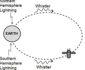
Fig. 1 Propagation of lightning whistler along magnetic field line in the plasmasphere.
study trends of “dispersion” which reflect the propagation characteristics of the lightning whistlers and compare them with those which are derived theoretically. The analysis shows that the source of whistler waves will easily deter-mine whether whistlers generated by lightning strikes are guided along the magnetic field lines from the southern or the northern hemispheres, as shown in Fig. 1 [13]. In ad-dition, studying the dispersion trend helps to determine the electron density profile in the Earth’s plasmasphere, because the propagation velocity of whistler mode waves depends on the intensity of the ambient magnetic field and the elec-tron density around the Earth [6], [14]. Therefore, it is im-portant to extrapolate the electron density profile of the en-tire plasmasphere by examining the dispersion trend along the spacecraft trajectory. For these reasons, we analyze the trend of the whistler dispersion in relation to parameters, particularly electron density profile in the plasmasphere. Fi-nally, we discuss whether the observed dispersion trends agree with the ones theoretically derived, and we show the feasibility of modeling the electron density profile using nu-merous datasets obtained by the WBA onboard Akebono.
2. Observation
In this study, we utilize the WBA waveform data observed by the WBA onboard Akebono. The WBA data were orig-inally recorded and stored in digital audio tapes (DATs). In the DATs, the analog time code signal, which indicates uni-versal time and date, is recorded on the left channel, while the measured waveform signal is recorded on the right chan-nel [1]. To analyze the data, it is necessary to playback the tape and converts it to waveform data represented by the waveform audio file format (WAV), digitizing by an A/D converter with a sampling frequency of 48 kHz. To gener-ate a plot showing the variation of frequency with time, we performed a Finite Fourier Transform (FFT) every 0.05 s. After FFT processing, we calibrated the spectrum based on the housekeeping data related to the autogain controller im-plemented in the WBA. We also eliminated spike noises that contaminated the waveform data. In the noise reduction pro-cess, we divided the 50 Hz–15 kHz band into 20 frequency ranges, then averaged the intensity of each frequency band,
Fig. 2 Detected lightning whistlers.
and subtracted neighboring frequency points. For the next step, we defined a threshold level for the detection of sig-nificant signals. If the intensity of differential data is larger than the threshold, it is considered to be a potential lightning whistler candidate. It is theoretically well known that Eck-ersley’s law [15] provides a simple relationship that defines the arrival timetof a lightning whistler at a frequency f as follows
t=D/f+t0 (1)
whereDis a constant called dispersion,tis the arrival time at frequency f, andt0is the time when the lightning strikes. Then, we applied an automatic algorithm to detect straight lines in a diagram in which the spectrogram is converted into
t in the horizontal axis and 1/f in the vertical axis. An example of lightning whistlers detected by this process is shown in Fig. 2, which is well marked by thick curves. The figure shows one of them symbolized byt1, f1,t2 and f2, wheret1andt2are the arrival times of the detected lightning whistler at frequencies of f1andf2, respectively.
Finally, we compute the dispersionDusing the follow-ing equation
D= 1t2−t1
√
f2 −
1 √
f1
(2)
By using Eq. (2), all dispersions of the detected lightning whistlers can be automatically enabled.
3. Dispersion Analysis
trajectory of Akebono.
In this section, we first theoretically describe the relationship between the dispersion and the propagation path length to show that the dispersion trend of lightning whistlers is useful for determining the plasma environment inside the Earth’s plasmasphere. As stated previously, the dispersion depends on several parameters, such as the inten-sity of the ambient magnetic field, the electron deninten-sity, and the path length along the propagation paths. The path length between the source point of lightning strikes and the obser-vation point in the Earth’s plasmasphere affects the disper-sion scale of lightning whistlers [9], [16]. Short path lengths lead to minimum dispersion, and vice versa [9], [16]. Fur-thermore, to estimate the path length, we can utilize a sim-ple method by assuming that the structure of the Earth’s magnetic field is approximated by a simple magnetic dipole model [17], [18]. By adopting the approximation, we can briefly calculate the path length of the lightning whistler to demonstrate why the dispersion changes along the trajectory of Akebono in such a manner.
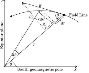
Using parameters such as the altitude and the latitude of the Akebono trajectory, it is possible to calculate the path length of each lightning whistler detected along the Akebono trajectories, assuming that each signal propagates along the magnetic field line of the Earth from the ground to the observation point. Note that whistler mode wave does not propagate strictly along the magnetic field line in ac-tual, but we assume here that the wave propagates along the magnetic field line with its wave normal angle parallel to the ambient magnetic field for simple calculation purposes. Then we analyze the approximated equation from a model of a dipole magnetic field line. Figure 3 shows a schematic picture of the magnetic field line at a given point in the plas-masphere. This figure shows the relationship between the geocentric distancerand the magnetic colatitudeθof any point on a field line [18]. In this case, letβbe the angle be-tween the magnetic field line and the latitude line. Bθ and
Brrepresent the horizontal component and the vertical
com-ponent of the magnetic field, respectively. The figure also shows the x-axis, which corresponds to the south
geomag-Fig. 3 Relationship between the radius vector and latitude of a field line.
netic pole of the Earth, while the y-axis corresponds to the equatorial plane of the Earth.
From the previous figure, the following equations can be derived:
Bθ=B0 1
r3sinθ (3)
Br=2B0 1
r3cosθ (4)
rdθ
dr ≈tanβ=
Bθ
Br
=1
2 sinθ cosθ=
1
2tanθ (5)
whereB0 is the equatorial surface magnetic field intensity of the Earth. After deriving the equations, we obtain the solution
cosβ= √ 2 cosθ
1+3 cos2θ (6)
To calculate the path length, we substitute (90+θ′) forθ, whereθ′is defined as the magnetic latitude. In accordance
with Fig. 4, we obtain the following equation
dr=cosβds=− 2 sinθ
′
1+3 sin2θ′
ds (7)
wheredsis an element of the path length along a magnetic field line. Then, the path length S is calculated using the following integration:
S =
ds=−
θ′
1
θ′
0
1+3 sin2θ′
2 sinθ′ dr (8)
We then consider a shell parameter L that corresponds to the distance, which is an intersection of the field line and the equatorial plane, and is given in units of Earth radii. Ac-cording to [18], [19],dris given by the following form
dr=−RE·L·2 cosθ′sinθ′dθ′ (9)
whereRE is the radius of the Earth, which is approximately
6371 km. Under these circumstances, the following equa-tion is derived.
S =
last equation to calculate the path length between the source point of the whistler wave and the spacecraft along the am-bient magnetic field line.
By using the equation, we can estimate each path length of the detected lightning whistler from the source point.
When an element of the path length is well defined, we can derive the lightning whistler dispersion along each propagation path theoretically. The propagation delay time
td, which is given by (t−t0) in Eq. (1), is expressed by using the following equation when the lightning whistler propa-gates along the ambient magnetic field line with its wave normal parallel to the magnetic field [20]
td=
tive index, wave frequency, plasma frequency, and electron gyrofrequency, respectively. Based on Eqs. (1) and (12), we can obtain the following equation
D= 1
When the wave frequency is significantly less than the local electron gyrofrequency, i.e., fc ≫ f, Eq. (13) is
approxi-mately described as follows
It is well known that the local electron plasma frequency is proportional toN1/2, whereNis the number density of elec-trons, and the local electron gyrofrequency is proportional to the geomagnetic field strengthB[20]. As was proposed by Carpenter and Smith [21], if the electron density in the plas-masphere is inversely proportional to the cube of the geo-centric distance as shown by Eq. (15) (hereafter we define this electron density profile as “Model 1”), we can obtain the following equations
whereN0are the electron density at upper ionosphere of the Earth. Combining Eqs. (14), (16), and (17), we obtain
D1∝
1
(1+3 sin2θ′)1/4ds (18)
whereD1is the dispersion at the observation point along the spacecraft trajectory when the electron density in the plas-masphere is represented by Eq. (15) (“Model 1”). By replac-ing in Eq. (18) by Eq. (7) and replacreplac-ingdrby Eq. (9), we can derive the dispersion using the following equation
D1∝
On the other hand, if the electron density in the plasmas-phere is, for example, given by Eq. (21) (hereafter we define this electron density profile as “Model 2”), which is known as gyrofrequency model [22], assuming that electron density is larger in the lower latitude region than the higher latitude region
N2=
N0
r31+3 sin2θ′ (21)
we can obtain the dispersion D2 by combining Eqs. (14), (17) and (21) as follows
D2∝
After the dispersions D1 andD2 are derived by assuming the electron density profile models, we introduce the typical observation events in which lightning whistlers are continu-ously observed along the trajectories of Akebono. We show the dispersion of these lightning whistlers has clear trend along the trajectory and we demonstrate that we can roughly estimate the electron density profile in the plasmasphere by comparing the observed dispersion trends with those theo-retically derived.
4. Result and Discussion
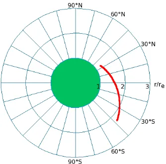
Figure 5 shows a train of lightning whistlers that lasted from 19:13 to 19:51 UT on March 20, 1991. Such lightning whistler trains occur because of the abundance of waves from the lightning strike detected by Akebono. The figure shows the dispersion trends of lightning whistlers, which descend when the time increases. The number of light-ning whistlers recorded during the time is 564, and the dis-persions vary between ∼12.81 and ∼4.194 Hz1/2s. In ac-cordance with the Akebono trajectory orbit, the lightning whistlers in the figure are detected along the Akebono tra-jectory between latitudes 47.83◦ (47,83◦N) and −11.09◦
(11.09◦S) and altitudes from ∼2232 to ∼7537 km, as
Fig. 5 Dispersion of lightning whistler observed on March 20, 1991.
Fig. 6 Altitude and latitude of Akebono on March 20, 1991.
Fig. 7 Dispersion of lightning whistler observed on July 12, 1989.
decreased gradually from∼49977 to∼10498 km. Because a decrease in the path lengths over time will decrease the dis-persion scale, this fact suggests that the waves of lightning whistler strikes propagate from the southern to the northern hemisphere.
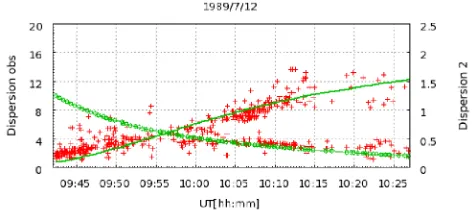
Figure 7 shows a train of lightning whistlers that oc-curred from 09:42 to 10:26 UT on July 12, 1989. The num-ber of lightning whistlers that were detected during that pe-riod of time was 542. The dispersions vary between∼1.11 and∼13.66 Hz1/2s. They were detected along the Akebono trajectory between latitudes 34.94◦ (34.94◦N) and−41.89◦
(41.89◦S) and altitudes from∼1420 to∼7911 km, as repre-sented in Fig. 8.
Two dispersion trends can be observed coincidentally in Fig. 7. The phenomenon occasionally occurred because lightning whistler sources originated from the southern and
Fig. 8 Altitude and latitude of Akebono on July 12, 1989.
the northern hemispheres and were detected simultaneously. As shown in Fig. 7, one has an ascending trend, while the other has a slightly descending trend. By using the altitude and latitude of the Akebono orbit, as shown in Fig. 8, we calculated the path lengths of lightning whistler waves that originated from both the northern and the southern hemi-spheres. Between 09:42 and 10:26 UT, the path lengths of lightning whistler waves originating from the northern hemisphere toward Akebono became larger from ∼1678 to ∼65849 km with increasing time. One of the disper-sion trends in Fig. 7 shows that the disperdisper-sion scale average was approximately∼2 Hz1/2s at 09:42 UT and gradually in-creased, becoming∼12 Hz1/2s at 10:26 UT.
In contrast, the path lengths of lightning whistler cal-culated from the source points in the southern hemisphere toward Akebono was∼21210 km at 09:42 UT while it was ∼8577 km at 10:26 UT. Another dispersion trend in Fig. 7 shows that the dispersion scale becomes smaller from an av-erage of∼6 Hz1/2s to
∼2 Hz1/2s from 09:42 to 10:26 UT. It can be conclusively stated that the ascending disper-sion trend in Fig. 7 shows waves of lightning whistler strikes propagate from the northern to the southern hemisphere. The other descending trend shows the waves of lightning whistler strikes propagate from the southern to the northern hemisphere. The VLF instruments onboard Akebono has a subsystem named PFX to determine wave normal direction and Poynting vector [1], but the measuring frequency be-ing set for PFX on this date was too high to detect lightnbe-ing whistlers and it was unfortunately impossible to determine the propagation direction of the whistlers.
propa-Fig. 9 Relationship between dispersion observed on March 20, 1991 (red symbols) and the one theoretically calculated by Model 1 (green line).
Fig. 10 Relationship between dispersion observed on March 20, 1991 (red symbols) and the one theoretically calculated by Model 2 (green line).
Fig. 11 Relationship between dispersion observed on July 12, 1989 (red symbols) and the ones theoretically calculated by Model 1 (green lines).
gate along a magnetic field line by cutting across the equa-torial plane over the time period from 19:13 to 19:42 UT, and they were detected in the northern hemisphere. After 19:42 UT, the lightning whistlers were detected in the south-ern hemisphere. In comparison, as shown in Fig. 9 when Akebono orbited in the further points from the source of lightning whistlers, the observed dispersion trend tends to deviate from the dispersion curve ofD1.
On the other hand, Fig. 10 shows the observed disper-sion trend and the line of disperdisper-sionD2theoretically calcu-lated by using Eq. (22). Also note that the scale forD2 is different from the observed dispersion. As seen in Fig. 10, the dispersionD2tends to slightly deviate away from the ob-served dispersion trend. However, it shows a better model than the one shown in Fig. 9.
Same analyses were applied to the event on July 12, 1989. Figure 11 shows the observed dispersion trends and two lines for the dispersionD1that calculated theoretically
Fig. 12 Relationship between dispersion observed on July 12, 1989 (red symbols) and the ones theoretically calculated by Model 2 (green lines).
by using Eq. (20). The “bullet” line represents decreasing dispersion and the “smooth” line indicates increasing dis-persion theoretically derived from Eq. (20). We can clearly observe that the bullet line appears like a curved line be-tween 09:42 and 09:56 UT. During this time, the lightning whistlers originated from the southern hemisphere and were detected in the northern hemisphere by cutting across the equatorial plane. After 09:56 UT, the dispersion D1looks like a straight line. As represented in Fig. 11, when Akebono orbited at lower altitudes in the earlier time, the dispersion
D1of the “bullet” line is not parallel with the observed dis-persion trend.
The smooth line in Fig. 11 appears to be almost a straight line. As stated previously, sources of lightning whistlers that correspond to increasing dispersion originate from the northern hemisphere and the observed dispersion trend also appears to be almost straight. The dispersionD1 of the “smooth” line is almost parallel with the observed dispersion trend.
Figure 12 shows the observed dispersion trends and the lines of dispersion D2 theoretically calculated by us-ing Eq. (22). Although the green lines have slight devia-tion from those of observed trends in the earlier times in the higher latitude region of northern hemisphere, they show a better model than the ones shown in Fig. 11.
5. Conclusion
In the present paper, we first showed that we can approx-imately derive the dispersion of lightning whistler and the electron density profile strongly affects the trend of disper-sion in the plasmasphere. Second, we introduced two typical events observed by Akebono in which lightning whistlers were continuously observed along the satellite’s trajectory. We demonstrated that the trends of dispersion of the light-ning whistlers basically give good agreement with the ones theoretically derived. We also showed that the calculated dispersions using the electron density profile of Model 2 was better fit to the observation results. As shown previ-ously, some deviations appeared because some parameters used when deriving the formula were assumed. In addition, it is also necessary to determine more precise propagation path using ray tracing technique and consider ionospheric contribution in deriving dispersion D. But our investiga-tion proved that analyzing the dispersion trends of lightning whistler observed in the plasmasphere is a powerful method to estimate global electron density profile in the plasmas-phere. As was described in the introduction, Akebono has continuously observed since 1989 and still in operation now, and enormous data of WBA waveform data is very valuable to study long term variation of electron density profile in the plasmasphere statistically.
Acknowledgments
We thank to our colleague Mr. Le Hoai Tam for his assis-tance in preparing the Akebono lightning whistler database.
References
[1] I. Kimura, K. Hashimoto, I. Nagano, T. Okada, M. Yamamoto, T. Yoshino, H. Matsumoto, M. Ejiri, and K. Hayashi, “VLF observa-tions by the Akebono (EXOS-D) satellite,” J. Geomag. Geoelectr., vol.42, pp.459–478, 1990.
[2] Y. Kasahara, A. Hirano, and Y. Takata, “Similar data retrieval from enormous datasets on ELF/VLF wave spectrum observed by Ake-bono,” Data Science Journal, vol.8, pp.IGY66–IGY75, March 2010. [3] J. Chum, F. Jirick, O. Santolik, M. Parrot, G. Diendorfer, and J. Fisr, “Assigning the causative lightning to the whistlers observed on satellites,” Annales Geophysical, vol.24, pp.2921–2929, Nov. 2006. [4] J. Oster, A.B. Collier, A.R.W. Hughes, L.G. Blomberg, and J. Lichtenberger, “Spatial correlation between lightning strikes and whistler observation and whistler observation from Tihany, Hun-gary,” South African Journal of Science, vol.105, pp.234–237, May/June 2009.
[5] D.L. Carpenter, “Remote sensing of the magnetospheric plasma by means of whistler mode signals,” Reviews of Geophysics, vol.26, no.3, pp.535–549, Aug. 1988.
[6] J. Crouchley, “A study of whistling atmospherics,” Aust. J. Phys., vol.17, pp.88–105, Aug. 1964.
[7] J.D. Menietti and D.A. Gurnett, “Whistler propagation in jovian magnetoshere,” Geophysical Research Letters, vol.7, no.1, pp.49– 52, Jan. 1980.
[8] G.J. Daniell, “Approximate dispersion formulae for whistler,” J. At-mospheric Terrestrial Physics, vol.48, no.3, pp.267–270, Aug. 1985. [9] R.L. Smith and J.J. Angeram, “Magnetospheric properties deduced
from OGO 1 observations of ducted and nonducted whistler,” J. Geo-physical Research, vol.73, pp.1–20, Jan. 1968.
[10] O. Santolik, M. Parrot, U.S. Inan, D. Buresova, D.A. Gurnett, and J. Chum, “Propagation of unducted whistlers from their source light-ning: A casestudy,” J. Geophysical Reserach, vol.114, pp.1–11, March 2009.
[11] J. Lichtenberger, C. Ferencz, D. Hamar, P. Steinbach, C. Rodger, M. Clilverd, and A. Collier, “Automatic retrieval of plasmaspheric electron densities: First results from automatic whistler detector and analyzer network,” General Assembly and Scientific Symposium, 2011 XXXth URSI, Aug. 2011.
[12] Y. Goto, Y. Kasahara, and T. Sato, “Determination of plasmas-pheric electron density profile by stochastic approach,” Radio Sci-ence, vol.38, no.3, 1060, doi:10.1029/2002RS002603, June 2003. [13] F. Akalin, D.A. Gurnett, T.F. Averkamp, A.M. Persoon, O. Santolik,
W.S. Kurth, and G.B. Hospodarsky, “First whistler observed in the magnetosphere of Saturn,” Geophysical Research Lett., vol.33, L20107, pp.1–5, 2006.
[14] R. Singh, A.K. Singh, and R.P. Singh, “Synchronized whistlers recorded at Varanasi,” Pramana J. Physics, vol.60, no.6, pp.1273– 1277, June 2003.
[15] D.A. Gurnett, W.S. Kurth, I.H. Cairns, and L.J. Granroth, “Whistler in Neptune’s magnetosphere: Evidence of atmospheric lightning,” J. Geophysical Research, vol.95, no.A12, pp.20,967–20,976, Dec. 1990.
[16] B.C. Edgar, “The upper and lower frequency cutoff of magneto-spherically reflected whistler,” J. Geophysicical Research, vol.81, pp.205–211, 1976.
[17] J.G. Luhmann and L.M. Friesen, “A simple model magnetosphere,” vol.84, pp.4405–4408, Aug. 1979.
[18] G.W. Prolss, Physics of the Earth’s space environment an introduc-tion, Springer, 2004.
[19] C.E. McIlwain, “Magnetic coordinates,” Space Science Reviews, vol.5, no.5, pp.585–598, 1965.
[20] D.L. Carpenter, “Electron-density variations in the magnetosphere deduced from whisler data,” J. Geophysical Research, vol.67, no.9, pp.3345–3360, Aug. 1962.
[21] D.L. Carpenter and R.L. Smith, “Whistler measurements of electron density in the magnetosphere,” Reviews of Geophysics, vol.2, no.3, pp.415–441, March 1964.
[22] R.L. Smith, “The use of whistlers in the study of the outer iono-sphere,” Tech. Rep. 6, Radioscience Lab., Stanford Univ., Stanford, Calif., Oct. 1960.
Yoshiya Kasahara received the B.E., M.E. and Ph.D. degrees in the field of electrical en-gineering from Kyoto University in 1989, 1991 and 1996, respectively. He had been a re-search associate of Kyoto University since 1992, and joined to Kanazawa University as an as-sociate professor in Department of Information and Systems Engineering in 2002. He is cur-rently a professor in Information Media Cen-ter, Kanazawa University. His research inter-ests are in radio engineering and radio science, intelligent signal processing for measurements of plasma waves onboard spacecraft, theoretical studies on generation and propagation mechanism of waves in space plasma, and database system for space environment. He is a member of Society of Geomagnetism and Earth, Planetary and Space Sciences (SGEPSS), Information Processing Society of Japan (IPSJ) and American Geophysical Union (AGU).