Economics of Education Review 18 (1999) 291–309
High school employment, high school curriculum, and
post-school wages
Audrey Light
*Department of Economics, The Ohio State University, 1945 North High Street, Columbus, OH 43210-1172, USA
Received 19 July 1997; accepted 15 November 1998
Abstract
The direct, skill-enhancing effect of high school employment is difficult to identify because high school work effort is correlated with curricular choices, postsecondary schooling and work effort, and many other observed and unobserved factors. This study uses data for male, high school graduates to estimate a wage model in which detailed measures of high school coursework and post-school work experience are included among the extensive array of covariates. Instru-mental variable methods are used to contend with the correlation between high school employment and unobserved characteristics. The direct effect of high school employment on subsequent wages proves to be small and relatively short-lived. Young men who work in high school gain additional, “indirect” wage benefits by taking vocational courses and gaining above-average work experience after graduation. 1999 Elsevier Science Ltd. All rights reserved.
Keywords:Work experience; Human capital; High school curriculum
1. Introduction
This study addresses a question that, despite its appar-ent simplicity, has yet to be answered satisfactorily by social scientists: Does holding a job while enrolled in high school enhance future labor market productivity? From a theoretical standpoint, high school employment has an ambiguous effect on career outcomes. It might give students a “leg up” in their careers by providing them with marketable skills, good work habits, and knowledge of the world of work. However, high school employment might indirectly hinder subsequent pro-ductivity by preventing students from learning as much in high school as they otherwise would. In light of the widely documented difficulties faced by many youth in transiting from school to a permanent, productive pos-ition in the labor force, it is important to know which effect dominates. Public policy can then be directed toward helping high school students gain employment
* Tel: 001 614 292 6701; fax: 001 614 292 3906; e-mail: [email protected]
0272-7757/99/$ - see front matter1999 Elsevier Science Ltd. All rights reserved. PII: S 0 2 7 2 - 7 7 5 7 ( 9 9 ) 0 0 0 0 7 - 2
(by providing job placement services, for example) or, as appropriate, toward discouraging such activities.
Efforts to identify the “value added” of high school employment are confounded by the fact that observed levels of work effort and scholastic achievement are cor-related with many factors. In deciding how to allocate their time between work and study, high school students are likely to weigh such factors as parental input and their own levels of ability and ambition. These same traits—as well as the choices made in high school—will also influence postsecondary schooling and labor supply decisions. By the time workers are observed several years after high school, their labor market productivity reflects the combined effects of innate factors, family background, labor market characteristics, and their entire schooling and employment histories. As a result, we can-not isolate the direct, skill-enhancing effects of high school employment on subsequent labor market out-comes without “netting out” the influences of many other factors, not all of which are observed.
“first generation” studies estimate simple, single-equ-ation models in which a particular academic or labor market outcome is expressed as a function of in-school work experience. Outcome measures that have been ana-lyzed include high school grade point averages or class rank (D’Amico, 1984; Greenberger & Steinberg, 1986; Lillydahl, 1990), high school completion or college attendance (Meyer & Wise, 1982; Marsh, 1991; Steel, 1991), post-high school employment or unemployment (Stevenson, 1978; Meyer & Wise, 1982; Marsh, 1991; Steel, 1991), post-high school wages or earnings (Stevenson, 1978; Stephenson, 1981; Meyer & Wise, 1982; Coleman, 1984; Ruhm, 1995) and post-high school occupational attainment or job benefits (Coleman, 1984; Ruhm, 1995). These studies typically control for a relatively small set of observed factors in addition to high school employment, and none contends with the inevitable correlation between high school employment and unobserved factors.1
Two recent studies address the shortcomings of the earlier literature by controlling for observed and unob-served sources of heterogeneity that, if ignored, might introduce a spurious correlation between high school employment and career outcomes. Ruhm (1997) esti-mates a number of single-equation models to assess the effect of high school employment on various outcomes (e.g., annual earnings, hourly wages, schooling attain-ment, and nonwage benefits) measured 6–9 years after high school. His primary strategy is to absorb other sources of observed heterogeneity that influence both high school employment decisions and subsequent career outcomes; he accomplishes this by including among his covariates an extensive array of family background and individual characteristics.2Hotz, Xu, Tienda and Ahituv (1998) abandon the single-equation approach in favor of a dynamic, discrete choice model. Every year from age 13 until the first year of full-time employment, individ-uals are assumed to choose one of six (year-long) states: school only, school plus part-time work, part-time work only, military service, full-time work, and other
activi-1See Ruhm (1997) for additional citations and a summary
of findings. As Ruhm notes, several of these studies can also be faulted for relying on nonrepresentative samples.
2Ruhm (1997) also uses two strategies, with varying success,
to control for the relationship between high school employment andunobservedfactors. A “treatment effects” model controls for unobserved factors affecting the decision to work while in school, but not the choice of employment intensity. An instru-mental variables approach controls for unobservables that are correlated with high school work intensity, but Ruhm’s IV esti-mators for the high school employment effect are imprecisely estimated and implausibly large (on the order of ten times larger than his other estimates), presumably because the instrumental variables do not explain enough variation in the endogenous covariate.
ties; wages are observed for each state that includes employment. The authors jointly estimate a wage model and the state choice models, allowing for correlations among the unobserved factors. This strategy enables them to identify the wage benefits of choosing “school plus work” net of any correlation between that particular choice and unobserved factors that also affect past choices and/or wages.
In the current study, I expand on the efforts of Ruhm (1997) and Hotz et al. (1998) to identify the true “value added” of high school employment on career outcomes. Using data for male respondents in the National Longi-tudinal Survey of Youth (NLSY)—the same data source used by both Ruhm and Hotz et al.—I estimate a human capital wage model in which log-wages earned on post-school jobs form the dependent variable and the covari-ates include measures of high school employment, high school achievement, post-school work experience and a host of labor market, job-related, family background, and personal characteristics. My goal is to determine whether tradeoffs exist between high school employment and high school achievement, and to identify the effect of each on estimated log-wage paths. I control for the con-founding effects of observed factors via my extensive array of covariates, and I also contend with potential cor-relation betweenunobservedfactors and my measures of high school employment, high school achievement, and post-school work experience. I do this by using a gen-eralized least squares, instrumental variables estimator similar to the one proposed by Hausman and Taylor (1981).
time-varying nature of the wage benefits associated with high school employment.
Third, I hold constant postsecondary schooling attain-ment and post-school work experience, which allows me to interpret my estimates using a standard, human capital framework. Ruhm observes career outcomes 6–9 years after high school, at which time respondents differ dra-matically with respect to their postsecondary schooling and work histories. He omits measures of schooling attainment and post-high school work experience from his set of covariates because they are endogenous, but as a result he cannot separate the productivity-enhancing effects of high school employment from the effects of subsequent schooling attainment and on-the-job train-ing.3I eliminate heterogeneity in postsecondary school-ing by limitschool-ing my sample to terminal high school gradu-ates, and I control for heterogeneity in post-school, on-the-job training with measures of actual and potential work experience. As noted above, I then contend with the endogeneity of work experience using an instrumen-tal variables approach.
A final difference between this study and its prede-cessors is that I explicitly consider the potential trade-off between high school employment and high school achievement. To control for high school achievement in my wage models, I use data on subject-specific credit hours earned by each respondent—information that is available because high school transcripts were collected and coded for a large number of NLSY respondents. Detailed transcript data are indispensable if we wish to assess the effect of high school employment on wages net of its effect on skills being learned contempor-aneously inside the classroom. In particular, these data enable us to investigate the presumption that employed high school students shun academic subjects in favor of such courses as typewriting, auto mechanics, and choir— curricula choices that may leave them with ample free time and even high grade point averages, but with poorer post-school wage earning capabilities than their nonem-ployed counterparts. This premise receives support in a recent study by Eckstein and Wolpin (1998), who use NLSY data to find a small, negative relationship between
3Ruhm’s approach is akin to identifying the returns to
schooling with a wage model that omits post-school experience from the covariates. Because schooling and work experience are strongly, positively correlated, such a model would imply much larger returns to schooling than are found in conventional models. To circumvent this difficulty, Ruhm presents one speci-fication in which the sample is confined to individuals who average at least 1000 h or 26 weeks of work during the period in which earnings are observed (6–9 years after high school). This is only a partial solution, for it still allows considerable variation in work effort within that window, as well as in the preceding years; in addition schooling attainment remains uncontrolled for.
high school work effort and the accumulation of credit hours. Neither Ruhm nor Hotz et al. include measures of high school achievement among their regressors, although a number of earlier studies use grade point averages or class rank as outcome measures in assessing the value of high school employment.
In the next section I explain how I select the sample of male high school graduates used throughout the study, and I provide a descriptive analysis of these respondents’ characteristics. In particular, I describe the extent of their high school employment experiences and summarize the relationships between high school employment and numerous other characteristics, including high school achievement. In Section 3 I describe the wage models to be estimated, define the covariates, and discuss the estimation technique. Section 4 presents the estimates, and in Section 5 I offer concluding remarks.
2. Data
2.1. Sample selection
The data are from the National Longitudinal Survey of Youth (NLSY), which began in 1979 with a sample of 12,686 males and females born in 1957–64. Respondents were interviewed annually from 1979 to 1994, at which time the survey became biennial. I use data from inter-view years 1979–91, and I restrict the analysis to a sub-sample of 685 males. Gender differences in high school employment are documented in Michael and Tuma (1984), Light (1995a), and Ruhm (1997), so in this paper I opt to focus exclusively on male workers. Further reductions in sample size are caused primarily by my requirements that (a) high school transcript data be avail-able for each respondent, (b) their labor market experi-ences be “observed” from the start of grade 11 onward, and (c) they receive no postsecondary schooling. In the remainder of this subsection I elaborate on the selection criteria and also describe the NLSY transcript and employment data.4
In 1980, 1981, and 1983 an attempt was made to col-lect high school transcripts for eligible NLSY respon-dents. Respondents were eligible if they consented to release their high school records, did not attend high schools outside the United States, and were not in the military subsample.5 In addition, respondents had to
4Additional information on the data can be found in US
Department of Labor (1998) and Light (1995b).
5The original NLSY sample of 12,686 respondents consisted
graduate from or otherwise exit high school before their transcripts were collected. Although more than 10,000 NLSY respondents were eligible for the transcript collec-tion in one of the three years, completed transcripts were acquired and coded for only 9010 respondents. I make an initial reduction in sample size by eliminating the 6283 female respondents, and also deleting 824 male members of the military subsample and an additional 1150 men for whom transcript data are unavailable. These deletions reduce the sample size to 4429.
I delete an additional 1082 men because they did not graduate from high school. Although the relationship between high school employment and the likelihood of graduation is a worthy subject for analysis (see D’Am-ico, 1984; Marsh, 1991; Eckstein and Wolpin, 1998), I choose to exclude high school dropouts so I can look at all respondents’ in-school employment experiences for two academic years prior to their school exit. If dropouts were included in the analysis, I would have to contend with the fact that they are legally barred from holding a job for most (or perhaps all) of their last two years of school.
The NLSY asks respondents about their work experi-ences with virtually every employer encountered from January 1978 onward or, for respondents who were not yet age 16 at that date, from age 16 onward. The reported information is used to create week-by-week variables on labor force status and hours worked on all jobs in pro-gress during the given week.6 To ensure that each respondent’s employment experiences are recorded from the start of grade 11 onward, I delete respondents from the sample if this date precedes January 1978; with few exceptions, all remaining respondents graduate from high school in the spring of 1980 or later. This leads to an additional 1561 respondents being dropped, and reduces the sample size to 1786.
I eliminate an additional 192 individuals because their transcripts are incomplete for grade 11 or 12. I require each respondent’s transcript to show at least four courses or four Carnegie credits for grades 11 and 12, where one Carnegie credit represents a year-long course.7I also eliminate 27 respondents who fail to report any employ-ment experiences during the 9 years following high school graduation. By observing career outcomes over a 9-year window I am able to identify changes over time in the wage effect of high school work experience. I choose 9 years as my cut-off because it corresponds to Ruhm’s (1997) 6–9 year outcome window, and because survey
6The arrays of weekly data are released as part of the NLSY
work history file.
7As part of the transcript collection effort, courses were
assigned three-digit codes identifying their content and credit hours were translated into Carnegie units. This was intended to produce uniformity across schools.
attrition reduces the number of respondents seen more than 9 years after their high school graduation date. A small number of respondents drop out of the NLSY prior to reaching the 9-year mark, in which case I simply observe them until their last interview date.
The deletion rules described above produce a sample of 1567 male respondents who graduate from high school and whose employment histories are recorded from the start of grade 11 onward. Many of these indi-viduals proceed to attend college and hold college jobs. The intervention of college attendance and employment complicates my efforts to identify the relationship between high school employment and subsequent wages, so I confine the sample to 685 terminal high school graduates—that is, respondents who report no postsec-ondary enrollment during the observation period. NLSY respondents are asked their enrollment status on a month-by-month basis from January 1980 onward (and in a more general manner prior to that date), so I can accurately identify even very short postsecondary enrollment spells for the respondents in my sample. I have replicated the entire analysis for the larger sample of 1567 respondents, and I summarize the key differ-ences between the two groups in subsequent sections.
2.2. Sample characteristics
In this subsection, I describe the amount of employ-ment experience acquired by the 685 sample members while enrolled in grades 11 and 12. I then segment the sample by high school work intensity and examine dif-ferences across groups in a large number of character-istics, including those related to high school achieve-ment. This descriptive analysis reveals a number of interesting contrasts between individuals who choose dif-ferent levels of high school employment effort, and it sets the stage for the regression analysis presented in subsequent sections.8
Table 1 describes the distribution of average hours worked per week during the 2 years preceding high school graduation. The 2-year period is broken down into four contiguous segments: the summer before grade 11, the grade 11 academic year, the summer before grade 12, and the grade 12 academic year. To measure average weekly hours of work, I count the total number of hours worked during each interim, and divide by the number of weeks elapsed. The average (and modal) durations of each academic year and summer are 36 weeks and 14 weeks, respectively. Each respondent’s employment history must be recorded from the onset of grade 11 in
8Most of the characteristics summarized in this section are
Table 1
Distribution of average hours worked per week in high school
Percent of individuals
Average hours worked per week Summer before Grade 11 Summer before Grade 12 Grades 11 and 12
grade 11 grade 12
0 27.9 41.6 26.7 29.3 22.8
1–10 37.4 24.8 15.9 20.3 34.7
11–20 14.7 17.4 22.3 20.0 25.1
211 20.0 16.2 35.0 30.4 17.4
Mean 12.3 8.5 15.7 13.4 10.3
(S.D.) (13.1) (10.9) (14.1) (13.2) (10.0)
Mean among workers 19.5 14.5 21.3 19.0 13.0
(S.D.) (11.5) (10.7) (12.3) (11.9) (9.6)
Number of individuals 515 685 685 685 685
order for him to remain in the sample, but employment during the summer preceding grade 11 is unknown for 25% of the sample.
Table 1 reveals that many high school juniors and seniors work a substantial number of hours during the academic year. The column titled “Grade 11” reveals that 41.6% of respondents do not work during their junior year of high school, while 24.8% average 1–10 h per week, 17.4% average 11–20 h per week, and the remain-ing 16.2% work more than 20 h per week durremain-ing the aca-demic year. As one would expect, employment is even more prevalent during the senior year of high school. The column titled “Grade 12” indicates that only 29.3% of sample members do not work during their senior year of high school, while 30.4% average over 20 h per week; the remaining respondents are evenly divided between working 1–10 and 11–20 h per week. The average num-ber of hours worked per week increases from 8.5 in grade 11 to 13.4 in grade 12; among those students who work, the average weekly effort increases from 14.5 h in grade 11 to 19.0 h in grade 12.9
Table 1 reveals the temporal patterns one expects to see in the employment of young people. In addition to a pronounced rightward shift in the distribution of average hours between the grade 11 and grade 12 academic years, there is also a rightward shift between the summer before grade 11 and the summer before grade 12. Young men are more likely to be employed as they age and,
9The patterns seen in Table 1 change very little when I use
a larger sample of 1567 men that includes college-goers. The only difference is that college-goers are slightly less likely than terminal high school graduates to work very intensively. In grade 12, for example, only 27.8% of the larger sample ages 21 or more hours per week of employment, and the aver-age work effort among workers falls from 19 to 17.7 h per week.
conditional on working, tend to increase their hours. However, there is not a monotonic increase in work effort over time, for high school students frequently work intensively during the summer and then cut back on their hours (or quit their jobs altogether) during the sub-sequent academic year. Nonetheless, it is relatively rare for young men to remain nonemployed throughout their last two academic years of high school. The right-most column of Table 1 shows that only 23% of the sample gains no work experience while enrolled in grades 11 and 12, while the typical student averages 10 h of work per week during this period of time.
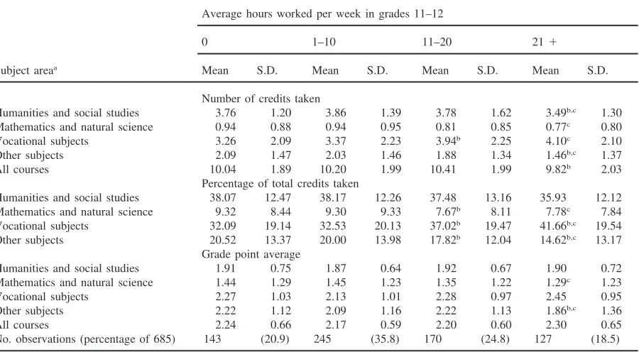
In Table 2, I categorize each sample member by the average number of weeks worked during the junior and senior academic years (0, 1–10, 11–20, or 211 h per week), and summarize the high school transcript data for respondents in each category. I confine my attention to the courses taken in grades 11 and 12, and I group the courses into four aggregate categories: humanities and social studies, mathematics and science, vocational, and all other courses. The five most frequently reported course titles in each category are listed in the note to Table 2.
Table 2 reveals a striking difference in the curricular choices of the four “types” of high school students: those who work the most intensively (211 h per week) take fewer academic courses and far more vocational courses than their counterparts who work moderately or not at all. Focusing first on the top panel of Table 2, we see that high school students who work 0–20 h per week take about 3.8 Carnegie credit hours in the humanities and social sciences, on average, while students who work over 20 h a week average only 3.5 Carnegie units. This statistically significant difference in means of about 0.3 Carnegie units represents roughly 50 fewer hours in the classroom over a 2-year period. Students in the 211
Table 2
High school credits and grade point average in each subject area by average hours worked per week in high school
Average hours worked per week in grades 11–12
0 1–10 11–20 211
Subject areaa Mean S.D. Mean S.D. Mean S.D. Mean S.D.
Number of credits taken
Humanities and social studies 3.76 1.20 3.86 1.39 3.78 1.62 3.49b,c 1.30
Mathematics and natural science 0.94 0.88 0.94 0.95 0.81 0.85 0.77c 0.80
Vocational subjects 3.26 2.09 3.37 2.23 3.94b 2.25 4.10c 2.10
Other subjects 2.09 1.47 2.03 1.46 1.88 1.34 1.46b,c 1.37
All courses 10.04 1.89 10.20 1.99 10.41 1.99 9.82b 2.03
Percentage of total credits taken
Humanities and social studies 38.07 12.47 38.17 12.26 37.48 13.16 35.93 12.12 Mathematics and natural science 9.32 8.44 9.30 9.33 7.67b 8.11 7.78c 7.84
Vocational subjects 32.09 19.14 32.53 20.13 37.02b 19.47 41.66b,c 19.54
Other subjects 20.52 13.37 20.00 13.98 17.82b 12.04 14.62b,c 13.17
Grade point average
Humanities and social studies 1.91 0.75 1.87 0.64 1.92 0.67 1.90 0.72
Mathematics and natural science 1.44 1.29 1.45 1.23 1.35 1.22 1.29c 1.23
Vocational subjects 2.27 1.03 2.13 1.01 2.28 0.97 2.45 0.95
Other subjects 2.22 1.12 2.09 1.16 2.22 1.13 1.86b,c 1.36
All courses 2.24 0.66 2.17 0.59 2.20 0.60 2.30 0.65
No. observations (percentage of 685) 143 (20.9) 245 (35.8) 170 (24.8) 127 (18.5)
aThe five most frequently reported course titles in each category, in descending order, are Humanities/Social Studies: American
History, English III, American Government, English IV; Popular Literature; Mathematics/Science: Chemistry I, Algebra II, Physics I, Geometry I, Biology; Vocational: General Work Experience, Typewriting I, Accounting, Automobile Mechanics, Auto Shop I; Other: Physical Education, Health, Band/Orchestra, Driver Education, Art I.
bThe null hypothesis that the difference between this mean and the one in the preceding column is zero is rejected at a 10%
signifi-cance level.
cThe null hypothesis that the difference between this mean and the one in the left-most column is zero is rejected at a 10%
signifi-cance level.
in mathematics and science courses than their less inten-sively employed counterparts, fewer credits in “other” subjects, and fewer credits overall. At the same time, they tend to take significantly more courses in vocational subjects such as “general work experience” (including off-campus internship programs), typewriting, and auto-mobile mechanics. The middle panel of Table 2 shows that students in the 211category devote 42% of their classroom time to vocational subjects, on average, which is far more than the other groups. As indicated by the superscripts in Table 2, the null hypothesis that the mean number of credits for the 211group is different than the nonworkers’ mean is rejected at a 10% significance level for all four subject areas.
The bottom panel of Table 2 shows that students who work 211 h per week tend to receive lower grades than their nonemployed counterparts in math, science, and “other” subjects, while performing slightly better in their vocational courses. The average grade point average in math and science falls from 1.44 to 1.29 as we read across Table 2, and the difference between the right-most and left-most means is statistically different than zero at
a 10% significance level. At the same time, the average grade point average in vocational subjects is almost 0.2 points higher for the most intensive workers than for the nonworkers. These statistics indicate that students tend to receive the highest grades in the subject areas where they take the most courses, presumably because they make curricular choices on the basis of aptitude. Interest-ingly, the grade point average for all courses taken in grades 11 and 12 does not differ significantly among the four “types” of students: the mean, overall GPA is between 2.2 and 2.3 for all four categories.10
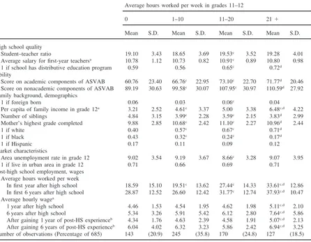
Table 3 extends Table 2 by showing how the four
10Adding college-goers to the sample produces three changes
Table 3
Characteristics of sample by average hours worked per week in high school
Average hours worked per week in grades 11–12
0 1–10 11–20 211
Mean S.D. Mean S.D. Mean S.D. Mean S.D.
High school quality
Student–teacher ratio 19.10 3.43 18.65 3.69 19.53c 3.52 19.28 4.01
Average salary for first-year teachersa 10.78 1.12 10.73 0.82 10.91c 0.89 10.80 0.98
1 if school has distributive education program 0.59 0.56 0.65c 0.72d
Ability
Score on academic components of ASVAB 60.76 23.40 66.76c 22.95 73.10c 22.70 71.77d 20.46
Score on nonacademic components of ASVAB 89.19 30.63 99.58c 30.07 107.95c 30.97 110.59d 27.92
Family background, demographics
1 if foreign born 0.06 0.03 0.06c 0.04
Per capita of family income in grade 12a 3.21 2.52 4.61c 3.37 5.00 3.38 6.48c,d 4.22
Number of siblings 4.84 3.15 3.99c 2.28 3.59c 2.15 3.83d 2.99
Mother’s highest grade completed 9.88 2.85 10.68c 2.42 11.10c 2.27 10.96d 2.44
1 if white 0.40 0.57c 0.67c 0.71d
1 if black 0.43 0.32c 0.24c 0.17d
1 if Hispanic 0.17 0.11 0.09 0.12
Market characteristics
Area unemployment rate in grade 12 9.02 3.54 9.19 3.67 8.66c 3.28 9.07 3.95
1 if live in urban area in grade 12 0.71 0.66 0.69 0.71
Post-high school employment, wages Average hours worked per week
In first year after high school 18.59 15.10 19.51c 13.62 27.44c 14.33 33.61c,d 12.86
In first 6 years after high school 28.87 12.52 26.60 12.42 31.77c 12.74 37.93c,d 10.47
Average hourly wagea
1 year after high school 4.46 1.53 4.54 1.95 4.62 1.98 5.11c,d 2.10
6 years after high school 5.34 3.26 5.91 5.42 6.12 2.80 7.64c,d 5.86
After gaining 1 year of post-HS experienceb 4.34 1.76 4.63 2.39 4.58 1.91 5.07c,d 2.13
After gaining 6 years of post-HS experienceb 6.04 4.02 6.32 3.23 5.86 2.42 6.94c,d 3.25
Number of observations (Percentage of 685) 143 (20.9) 245 (35.8) 170 (24.8) 127 (18.5)
aIn 1982 dollars. All but average hourly wage are divided by 1000.
b1800 h of cumulative, post-high school work experience is defined as 1 year.
cThe null hypothesis that the difference between this mean and the one in the preceding column is zero is rejected at a 10%
signifi-cance level.
dThe null hypothsis that the difference between this mean and the one in the left-most column is zero is rejected at a 10%
signifi-cance level.
“types” of individuals differ in terms of their high school, family, and personal characteristics, as well as in their post-secondary employment and wages. The top rows, which summarize characteristics of the respon-dents’ high schools, reveals that typical measures of high school quality (student–teacher ratio and average teacher salary) do not differ systematically across the four categ-ories. Students who work intensively in high school are neither more nor less likely than their less employed classmates to attend “good” schools. However, their high schools are far more likely to have distributive education programs, which are designed to combine classroom training with internships and other forms of “real world” experiences. Over 70% of the students who average more
than 20 h of work per week have access to such pro-grams, while fewer than 60% of the less intensively employed students do so. This correlation is unsurpris-ing, for one would expect distributive education pro-grams to facilitate the entry of high school students into the labor market.
to obtain the “academic” score, while the “nonacademic” score is the sum of the raw scores for the numerical oper-ations, coding speed, auto and shop information, mech-anical comprehension, and electronics information tests. As Table 3 shows, mean scores on both the academic and nonacademic portions of the ASVAB increase sig-nificantly as we move from the nonworkers to the stu-dents who average 1–10 h per week, and again as we move from the 1–10 category to the 11–20 category. The upward trend then levels off, with the two most intensive employment categories exhibiting mean scores that are statistically indistinguishable.
Among the family background, demographic, and market characteristics considered in Table 3, a number of interesting contrasts emerge. First, there is a clear, positive relationship between high school employment intensity and per capita family income: students who do not work in grades 11 and 12 come from families with an average, annual income of US$3210 per capita, while those who average over 20 h per week have an average, annual, per capita family income of US$6480. One explanation for this pattern is that the money earned on jobs held in high school contributes to family income. A more likely explanation is that students who work tend to come from families where one or more parents work continuously throughout the year. Students from such families may learn about employment opportunities from their employed parents or even obtain jobs at their par-ents’ work places. Second, studpar-ents’ work efforts are also positively correlated with their mothers’ (and, although it is not reported in Table 3, fathers’) schooling attainment. Parental schooling is positively correlated with parental employment level and earnings, so this pat-tern is consistent with the preceding one. Third, race and high school employment are strongly related. Among the 143 males who do not work at all during grades 11 and 12, 40% are nonblack, non-Hispanic (henceforth referred to as “white”), 43% are black, and the remaining 17% are Hispanic. Among individuals averaging more than 20 h of work per week, 71% are white and only 17% are black. This pattern is consistent with the well known finding that young, black men are more likely than non-blacks to be nonemployed. Such patterns are generally attributed in part to the fact that blacks are concentrated in economically depressed urban areas where jobs are scarce, but Table 3 shows that nonemployed high school males do not differ significantly from others in their tendency to live in urban areas or in locales with above-average unemployment rates.
The bottom rows of Table 3 reveal that high school employment intensity is positively related to post-high
11The ASVAB was administered to virtually all NLSY
respondents in the summer and fall of 1980, when the members of my sample were still in high school or had just graduated.
school employment. The typical male who averages more than 20 h of work per week during high school works an average of 34 h per week in the following year and 38 h per week in the following 6 years. This is sub-stantially more work effort than is seen among the “inter-mediate” workers and especially the nonworkers, who average only 19 h per week in the year after high school. Individuals who work 21 1 h a week in high school also tend to earn higher wages than their less employed counterparts when a fixed amount of post-graduation time has elapsed. One year after graduation, for example, their average wage is US$5.11/h, versus about US$4.50/h for the other groups. There are also statisti-cally significant, but smaller, differences in mean wages among these “types” of students when the amount of actual, post-high school work experience (as opposed to time elapsed, or “potential” work experience) is held constant.
3. Wage model
The summary statistics shown in the preceding section demonstrate systematic relationships between hours worked in high school and subsequent wages, as well as a large number of characteristics that are likely to influ-ence wages. Because high school employment is corre-lated with so many wage determinants, it is apparent that one must proceed carefully in identifying the marginal, skill-enhancing effect of high school employment on subsequent wages. In this section I describe the wage model used to identify the effects of interest, define the covariates, and describe the IV/GLS estimation pro-cedure used to handle the endogeneity issues discussed in the introduction.
To identify the wage effects of high school employ-ment, I model post-high school wages as follows:
lnWit5b11b2HSXi1b3HSAi1b4HSQi (1)
1b5Ai1b6MKTit1b7EXPit1ai1eit
whereWitis the average hourly wage earned by individ-ualiat timetduring the period after high school gradu-ation. Eq. (1) assumes post-high school wages depend on high school work experience (HSX), high school achievement (HSA), high school quality (HSQ) and ability (A), none of which vary during the post-high school period. The next term in Eq. (1), MKT, represents market characteristics prevailing at the time the wage is paid; in practice, MKT can be expanded to include demographic and job-related factors (e.g., union status) that also influence wages or skill accumulation. EXP rep-resents post-high school work experience, and also varies over time. The remaining terms in Eq. (1), aiand eit,
Because Eq. (1) represents a twist on conventional human capital earnings functions, it is worth comparing it to the following, more orthodox model:
lnWit5g11g2Si1g3Ai1g4MKTit1g5EXPit (2)
1hit
Eq. (2) resembles specifications used by Hanoch (1967) and Mincer (1974) in their pioneering empirical studies, and by legions of subsequent researchers who share their “human capital” approach to analyzing life-cycle wage paths. As is well known, the rationale for Eq. (2) is that wages are tied to the amount of marketable skill embodied by workeriat timet. Baseline or innate skill levels are captured byA, or measured ability, although analysts often omitAfor lack of data.12Years of school-ing (S) control for skills obtained during the pre-employ-ment portion of the life-cycle when individuals devote all their effort to skill acquisition. EXP, which may mea-sure years since school exit or, ideally, actual work experience gained during that period, controls for skills obtained via on-the-job training subsequent to school exit. MKT and h represent additional sources of observed and unobserved heterogeneity.
The covariatesA, MKT and EXP play the same roles in my model (Eq. (1)) as in Eq. (2). I eliminateSin Eq. (1) because my sample is homogeneous with respect to schooling attainment. However, it has long been recog-nized that a measure of “education”—what is actually learned in school—is desired in models such as Eqs. (1) and (2), and not simply measures of school quantity. Thus, I control for school quality (HSQ) and student achievement (HSA) in Eq. (1) to capture differences in “education” among my sample of terminal high school graduates.13 The remaining term in model (1), high school experience (HSX), is the key covariate in my analysis and the most significant departure from the orthodox model (2). Whereas model (2) does not acknowledge a “transition period” during which individ-uals combine work and school, my model does. By con-trolling for HSX, I explicitly account for the fact that individuals who have not begun their post-school careers
12Even when test scores and other ability measures are
avail-able, as they are in the NLSY, it is unclear whether they meas-ure innate ability.
13Welch (1966) was among the first to examine the link
between school quality and subsequent earnings; Betts (1995) is an example of a more recent, NLSY-based study of school quality. Rumberger and Daymont (1984), Altonji (1995) and Levine and Zimmerman (1995) are among the small number of studies that examine the effect of academic achievement (as measured by course work) on subsequent wages.
might possess varying levels of marketable skill as a result of their in-school labor market experiences.14
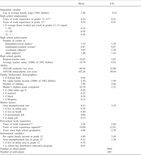
The dependent variable (lnW) used to estimate Eq. (1) is the natural logarithm of the CPI-deflated, average, hourly wage (in 1982 dollars) earned on jobs held during the 9 years following high school graduation. The NLSY reports wages and other job-related characteristics for virtually all employment spells encountered by respon-dents, with the exception of jobs lasting less than 2 months. Multiple (annual) wages are reported for jobs that span adjacent interview dates, while a single wage is reported for shorter jobs. The sample used to estimate Eq. (1) contains 5689 observations for 685 men, and con-sists of all wages reported during the 9 years following each respondent’s high school graduation date. Summary statistics for the dependent variable, as well as for the covariates described below, appear in Table 4.
To construct a measure of high school work experi-ence (HSX) for inclusion in Eq. (1) I must summarize the employment data described in Table 1 in a parsi-monious, yet meaningful, way. The variable I use for much of the analysis measures the cumulative number of hours worked during the junior and senior academic years. I divide this cumulative measure by 1800 to con-vert it to “one-year” units; an individual who averages 25 h of work per week for two, 36-week long academic years is considered to earn one year of high school work experience. To allow for nonlinearities in the wage effects of high school work experience, I also use an alternative measure of HSX consisting of three dummy variables indicating whether the average number of hours per week worked in grades 11–12 is 1–10, 11–20, or 21 or more; no employment is the omitted group. To allow the wage effects of high school experience to vary over time, I interact my continuous measure of HSX with a series of dummy variables indicating the number of years since high school graduation. This unrestricted spline function allows the relationship between high school experience and log-wages to change over time in a very flexible manner.
My decision to use work experience accumulated throughout the junior and senior years of high school as my measure of HSX requires some justification, especially in light of Ruhm’s (1997) conclusion that senior-year employment affects subsequent career out-comes but earlier work experience does not. I “start the
14To develop a formal model of optimal, life-cycle human
Table 4
Means and standard deviations of variables used in wage models
Mean S.D.
Dependent variable
Log of average hourly wage (1982 dollars) 1.60 0.43
High school employment
Years of work experience in grades 11–12a,b 0.44 0.41
Years of work experience in grade 12a,c 0.56 0.53
1 if average hours worked per week in grades 11–12 equals
1–10a 0.35
11–20a 0.26
211a 0.20
High school achievement Number of credits in
humanities/social studiesa 3.74 1.29
mathematics/natural sciencea 0.87 0.87
vocational subjectsa 3.65 2.20
other subjectsa 1.88 1.42
High school quality
Student–teacher ratio 19.07 3.67
Average teacher salary (1000s of 1982 dollars) 10.79 0.92
Ability
ASVAB academic test score 68.46 22.80
ASVAB nonacademic test score 102.26 30.64
Family background, demographics
1 if foreign born 0.04
Per capita family income (1000s of 1982 dollars) 2.50 1.99
Number of siblings 3.96 2.60
Mother’s highest grade completed 10.70 2.51
1 if child under age 6 0.26
1 if married 0.25
1 if black 0.28
1 if Hispanic 0.12
Market factors
Area unemployment rate 8.43 3.29
1 if live in urban area 0.70
1 if live in South 0.40
1 if government job 0.06
1 if union job 0.15
Post-school work experience
Years of work experiencea,d 3.58 2.60
Years of work experience squareda,d 19.60 23.91
Years since high school graduation 4.06 2.29
Instrumental variablese
Per capita family income in grade 12 4.80 3.49
Area unemployment rate in grade 12 8.32 3.38
1 if live in urban area in grade 12 0.70
1 is school has distributive education program 0.62
Number of observations 5689
Number of individuals 685
aEndogenous variable.
bCumulative hours worked in grades 11–12 divided by 1800. cCumulative hours worked in grade 12 divided by 900.
clock” on workers’ high school employment experiences at the start of the junior year because most students are legally barred from entering the work force until shortly before that date. My primary reason for using a cumulat-ive measure of junior- and senior-year experience is that there is no a priori reason to control for one and not the other. Just as orthodox wage models control for cumulat-ive work experience gained since the start of the career, my measure of “pre-career” experience treats all years identically. Moreover, I lack compelling statistical evi-dence that the junior and senior years should be treated differently. Following Ruhm (1997), I estimate a version of Eq. (1) in which junior- and senior-year work experi-ences are controlled for separately. The estimated coef-ficient for junior-year employment is about 30% smaller than the one for senior-year employment, but because both are estimated imprecisely (due to a high degree of correlation between the two variables) I cannot reject the null hypothesis that the two coefficients are equal.15 Although my preferred measure of high school employ-ment is cumulative hours worked in grades 11–12, for comparability with Ruhm’s analysis I also present results based on a measure of senior-year employment only.
The measures of high school achievement (HSA), high school quality (HSQ) and ability (A) in Eq. (1) are ident-ical to variables summarized in the preceding section. I control for high school achievement with four variables measuring the cumulative number of Carnegie credits accumulated during grades 11 and 12 in four subject areas: humanities and social studies, mathematics and science, vocational subjects, and other subjects. High school quality is measured by the student–teacher ratio
15Ruhm (1997) reports similar findings, but draws
con-clusions that differ from mine. For example, he reports coef-ficients (in the bottom panel of column b of his Table 4) that imply roughly 9% and 16% wage premia associated with 10 h per week of employment in the junior and senior years, respect-ively. Thep-values for the junior- and senior-year coefficients are 0.243 and 0.002, so he opts to omit junior-year employment from the model because the 9% return is not statistically dis-tinguishable from 0%.
It is worth noting that another difference between Ruhm’s analysis and mine is that he uses “reference week” employment as his primary measure of high school work experience, while my measure comes from the week-by-week employment data in the work history file. Ruhm also experiments with the work history data but argues that they are likely to be error-ridden because they require respondents to recall their employment experiences over a (roughly) one-year retrospective. Research on retrospective recall in the NLSY and other longitudinal sur-veys (e.g., Duncan & Hill, 1985; Dugoni et al., 1997) does not indicate that the NLSY work history data are likely to be unduly error-ridden. In fact, I am concerned that “reference week” data do not accurately measure employment throughout the aca-demic year for respondents who vary their work effort over time.
in the respondent’s high school, as well as the average annual salary (in thousands of CPI-deflated, 1982 dollars) paid to first-year teachers. These values are obtained directly from schools as part of the NLSY high school survey, but are missing for about 15% of obser-vations. I set missing observations equal to the sample mean and define two dummy variables indicating miss-ing high school quality data. To control for student ability, I use respondents’ scores on both the academic and nonacademic portions of the ASVAB (see Section 2 for details).
The covariate vector MKT in Eq. (1) includes not only market-related factors, but also family background and personal characteristics that are likely to influence both in-school and post-school skill acquisition. These vari-ables, along with the measures of post-school experience (EXP) are fairly standard in wage models such as (1) and (2). I control for family and personal characteristics with dummy variables indicating the respondent is foreign born, black, or Hispanic (with black, non-Hispanic the omitted race group), and with continuous measures of his number of siblings in 1979 and his mother’s highest grade of school. While these variables are time-invariant, I also control for three factors meas-ured at time t: per capita, family income net of the respondent’s annual labor earnings, whether he is mar-ried, and whether his household contains children under age 6. Because family income and mothers’ schooling levels are unreported for 6% and 7% of all observations, respectively, I include “missing” dummies for those two variables. To control for market characteristics at timet, I include the unemployment rate in the respondent’s local labor market, and I also include dummy variables indicating whether he lives in an urban area or in the South, whether he works in the public sector, and whether his job is unionized. My measures of post-school work experience include the number of months since high school graduation divided by 12 (“potential” experience) and the number of hours worked between high school graduation and time t divided by 1800 (“actual” experience) and its square. I control for both actual and potential experience to contend with the unemployment and nonemployment that characterize the careers of young men. In a group of individuals with the same amount of post-school work experience, those who have been out of school the longest have spent the most time nonemployed and are likely to earn less than their more continuously employed counterparts.
I assume the time-invariant, person-specific compo-nent of the error term in Eq. (1) (ai) and the time-varying
component (eit) are distributed with zero means and
con-stant variances equal to s2
a and s2e , respectively. I assumeeitis orthogonal toaiand each of the covariates
in Eq. (1), butai is likely to be correlated with HSX,
allo-cation decisions are affected by factors that cannot be observed. By assuming these unobservables are time-invariant, I am able to formally address the endogeneity issues discussed in the introduction.16
To contend with the potential correlation betweenai
and HSX, HSA and EXP, I estimate the parameters in Eq. (1) using a variant of the instrumental variables, gen-eralized least squares (IV/GLS) method proposed by Hausman and Taylor (1981). Following Hausman and Taylor, the “core” instruments consist of deviations from within-person means of each time-varying regressor, plus the within-person means of each exogenous regressor. Given my assumptions about the error struc-ture of Eq. (1), each of these variables is orthogonal to bothaiandeit and is, therefore, a valid instrument. To
improve theR2in the first-stage regressions for HSX and HSA, I also use four additional instruments: per capita, family income during the respondent’s senior year of high school, the unemployment rate in his local labor market during that year, a dummy variable indicating whether he lives in an urban area during that period, and a dummy indicating whether his high school offers a dis-tributive education program. All four variables (which are summarized in Tables 3 and 4) help explain high school employment decisions, but should be orthogonal to the error terms in Eq. (1). Because I include among the covariates in Eq. (1) family income, unemployment rates, and urban status measured at timet, I am relying on intertemporal variation in these variables (due partly to post-high school geographic mobility) for identifi-cation. The addition of the four “extra” instrumental vari-ables increases theR2in the first-stage regressions by a nontrivial amount (e.g., from 0.26 to 0.32 in a typical regression), and I reject at a 5% significance level the null hypothesis that these four instruments belong in the second-stage regression.
4. Findings
The goal of my econometric analysis is to identify the “value added” of high school employment, by which I mean its effect on subsequent wages net of any corre-lation with other factors that influence wages. Only by identifying the “value added” can we determine whether high school employment has a direct effect on labor mar-ket productivity. I believe IV/GLS estimation of wage model (1) is an appropriate way to achieve this goal
16ASVAB scores, union membership and marital status are
also likely to be correlated with unobserved, personal character-istics. However, my estimated coefficients for HSX and HSA are not sensitive to assumptions about the endogeneity of these covariates, so I treat them as exogenous.
because the model controls for numerous sources of observed heterogeneity and also contends with corre-lation between high school employment and personal characteristics that remain unobserved. In this section, I present IV/GLS estimates of (1) as well as estimates of alternative specifications that reveal how inferences about the “value added” of high school employment are affected by the failure to control for observed and unob-served sources of heterogeneity.
In Table 5, I present estimated coefficients from alter-native specifications of my wage model. Column head-ings 1 through 12 refer to alternative specifications that vary in terms of the measure of high school work experi-ence and the inclusion of other covariates (HSA and EXP). For each specification I present both IV/GLS and GLS estimates; the latter account for the nonspherical nature of the disturbances due to each respondent con-tributing multiple wage observations to the sample, but assume the disturbances are unrelated to each covariate. Table 5 contains estimated coefficients for the high school employment (HSX) covariates only; estimated coefficients for the remaining covariates for selected specifications appear in Tables 6 and 7.17
I begin by discussing the estimates for specifications 1–3, each of which controls for high school work experi-ence with a single, cumulative measure of the number of hours worked in grades 11 and 12 (divided by 1800). These specifications are quite restrictive in that they con-strain the relationship between hours worked in high school and log-wages to be linear. Specification 1 omits both HSA and EXP, which meansb3andb7in Eq. (1) are constrained to be zero. Specification 2 includes EXP among the covariates, and specification 3 controls for both HSA and EXP. I do not show results of experiments in which A and HSQ are excluded from the model because their presence proves to have an insignificant effect on the estimated coefficients for high school work experience, although they help explain the variation in log-wages.
Table 5 reveals that when GLS is used to estimate specification 1—that is, when I assume that the residuals are orthogonal to all included covariates—the estimated coefficient for high school employment is 0.075, with a standard error of 0.021. This implies that an individual who averages 25 h per week throughout his junior and senior years of high school subsequently earns 7.5% higher wages during the entire 9-year observation period than an individual who was nonemployed in high school. An individual who works only 10 h per week in grades 11 and 12 accumulates 720 h of work experience, or 0.4 years, and receives a 3% wage premium. When I
esti-17The estimated coefficients for the covariates listed in
Table 5
Estimated coefficients for selected covariates in alternative specifications of wage model
GLS IV/GLS
1 2 3 1 2 3
Years of work experience in grades 0.075 0.033 0.030 0.146 0.068 0.062 11–12
(0.021) (0.014) (0.014) (0.068) (0.021) (0.021)
4 5 6 4 5 6
Years of work experience in grade 12 0.064 0.026 0.024 0.122 0.055 0.051 (0.017) (0.011) (0.011) (0.052) (0.016) (0.016)
7 8 9 7 8 9
1 if average hours worked per week in grades 11–12 equals
1–10 0.004 0.019 0.018 0.003 0.015 0.012
(0.023) (0.022) (0.022) (0.081) (0.077) (0.077)
11–20 0.004 0.016 0.021 0.061 0.046 0.046
(0.026) (0.025) (0.025) (0.088) (0.083) (0.085)
211 0.087 0.053 0.049 0.102 0.071 0.059
(0.028) (0.026) (0.025) (0.063) (0.057) (0.048)
10 11 12 10 11 12
Years of work experience in grades 11–12 interacted with dummy variable indicating years since high school graduation equals
1 0.035 0.035 0.034 0.073 0.033 0.030
(0.031) (0.031) (0.032) (0.045) (0.046) (0.045)
2 0.028 0.025 0.023 0.063 0.019 0.020
(0.031) (0.031) (0.030) (0.041) (0.040) (0.040)
3 0.094 0.066 0.060 0.094 0.041 0.038
(0.030) (0.030) (0.030) (0.040) (0.039) (0.039)
4 0.082 0.062 0.059 0.084 0.042 0.042
(0.029) (0.028) (0.027) (0.038) (0.041) (0.040)
5 0.088 0.061 0.058 0.109 0.028 0.038
(0.029) (0.029) (0.028) (0.039) (0.030) (0.030)
6 0.164 0.058 0.054 0.173 0.065 0.059
(0.029) (0.028) (0.027) (0.042) (0.030) (0.029)
7 0.128 0.044 0.049 0.194 0.050 0.045
(0.030) (0.031) (0.030) (0.046) (0.033) (0.032)
8 0.166 20.031 20.028 0.220 20.016 20.005
(0.041) (0.051) (0.050) (0.050) (0.053) (0.055)
9 0.170 20.048 20.036 0.226 20.017 20.001
(0.100) (0.060) (0.060) (0.152) (0.063) (0.059)
Control for post-high school work no yes yes no yes yes
experience
Control for high school course credits no no yes no no yes
Note: Standard errors are in parentheses. Additional GLS and IV/GLS estimates for specifications 3, 9, and 12 appear in Tables 6 and 7.
mate the identical model using the IV/GLS procedure described in Section 3 (with high school employment as the sole endogenous variable), the estimated coefficient almost doubles to 0.146. The difference between the GLS and IV/GLS estimates suggests that high school
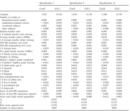
Table 6
Additional GLS estimators for selected wage models summarized in Table 5
Specification 3 Specification 9 Specification 12
Coeff. (S.E.) Coeff. (S.E.) Coeff. (S.E.)
Constant 1.052 0.130 1.018 0.130 1.100 0.130
Number of credits in
humanities/social studies 0.006 0.007 0.008 0.007 0.005 0.006
mathematics/natural science 20.034 0.010 20.033 0.010 20.033 0.009
vocational subjects 0.007 0.002 0.007 0.002 0.006 0.003
other subjects 20.008 0.006 20.007 0.006 20.008 0.006
Student–teacher ratio 0.005 0.002 0.005 0.002 0.004 0.002
1 if student–teacher ratio missing 0.020 0.029 0.028 0.028 0.018 0.028
Average teacher salary (1000s) 0.018 0.009 0.020 0.009 0.018 0.008
1 if average teacher salary missing 20.015 0.029 20.021 0.028 20.013 0.028
ASVAB academic test score 0.001 0.001 0.001 0.001 0.001 0.000
ASVAB nonacademic test score 0.001 0.000 0.001 0.001 0.001 0.000
1 if foreign born 20.025 0.042 20.018 0.042 20.024 0.041
Per capita family income (1000s) 0.009 0.003 0.008 0.004 0.008 0.002
1 if family income missing 20.044 0.040 20.041 0.040 20.045 0.040
Number of siblings 20.002 0.003 20.003 0.003 20.002 0.003
Mother’s highest grade completed 0.001 0.004 0.003 0.005 0.003 0.003
1 if mother’s highest grade missing 20.021 0.030 20.024 0.029 20.019 0.029
1 if child under age 6 0.008 0.015 0.010 0.015 0.008 0.015
1 if married 0.044 0.015 0.044 0.015 0.044 0.014
1 if black 0.011 0.024 0.010 0.025 0.011 0.023
1 if Hispanic 0.056 0.030 0.054 0.029 0.057 0.029
Area unemployment rate 20.012 0.002 20.013 0.002 20.012 0.002
1 if live in urban area 0.020 0.015 0.019 0.015 0.019 0.014
1 if live in South 20.018 0.016 20.018 0.016 20.020 0.016
1 if government job 20.022 0.023 20.020 0.024 20.022 0.022
1 if union job 0.231 0.015 0.232 0.015 0.229 0.015
Years of post-HS experience 0.084 0.009 0.084 0.009 0.081 0.008
Years of post-HS experience squared 20.004 0.001 20.004 0.001 20.003 0.000 Years since high school graduation 20.010 0.008 20.010 0.008 20.012 0.002
s2
a 0.052 0.052 0.051
s2
e 0.126 0.126 0.125
Root mean squared error 0.328 0.327 0.325
Number of observations 5689 5689 5689
Note: Each specification also includes dummy variables indicating the calendar year (1981–91).s2
aands2eare the estimated variances
of the individual and transitory components of the residual.
direct effect of high school employment to be under-stated relative to the preferred IV/GLS estimate.
Specification 2 is identical to 1 except it also controls for three measures of post-school work experience: time elapsed since high school graduation and hours of actual work experience (divided by 1800) and its square. Table 5 indicates that the addition of these three variables has a dramatic effect on the estimated coefficient for high school employment. The GLS estimate falls to 0.033 and the IV/GLS estimate falls to 0.068; both are less than half as large as the corresponding estimates for specifi-cation 1.18 Because high school employment and post-school employment are strongly, positively correlated (as
shown in Table 3), omission of the latter causes the effect of high school work experience to be overstated. The large estimated effect in specification 1 reflects the direct, skill-enhancing effect of high school employment on subsequent wagesplusthe indirect effect of its corre-lation with subsequent work effort. The latter effect is important, for it suggests that high school employment may foster good work habits, impart job-seeking skills, and otherwise enhance the post-school work continuity
18High school employment and actual experience and its
Table 7
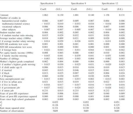
Additional IV/GLS estimators for selected wage models summarized in Table 5
Specification 3 Specification 9 Specification 12
Coeff. (S.E.) Coeff. (S.E.) Coeff. (S.E.)
Constant 1.062 0.130 1.001 0.140 1.158 0.131
Number of credits in
humanities/social studies 0.006 0.007 0.009 0.007 0.004 0.006
mathematics/natural science 20.033 0.010 20.033 0.010 20.034 0.009
vocational subjects 0.006 0.004 0.006 0.004 0.007 0.005
other subjects 20.007 0.007 20.005 0.007 20.010 0.006
Student–teacher ratio 0.004 0.002 0.005 0.002 0.004 0.002
1 if student–teacher ratio missing 0.015 0.029 0.032 0.031 0.020 0.028
Average teacher salary (1000s) 0.018 0.009 0.021 0.009 0.020 0.008
1 if average teacher salary missing 20.014 0.029 20.026 0.031 20.011 0.028
ASVAB academic test score 0.001 0.001 0.001 0.001 0.000 0.000
ASVAB nonacademic test score 0.001 0.000 0.001 0.000 0.001 0.000
1 if foreign born 20.022 0.043 20.011 0.044 20.023 0.042
Per capita family income (1000s) 0.008 0.003 0.008 0.003 0.010 0.002
1 if family income missing 20.043 0.041 20.039 0.041 20.051 0.040
Number of siblings 20.003 0.003 20.003 0.004 20.002 0.003
Mother’s highest grade completed 0.002 0.004 0.000 0.004 0.000 0.003
1 if mother’s highest grade missing 20.015 0.030 20.025 0.031 20.020 0.029
1 if child under age 6 0.006 0.015 0.010 0.016 0.010 0.015
1 if married 0.045 0.015 0.046 0.015 0.041 0.015
1 if black 0.013 0.025 0.007 0.025 0.004 0.024
1 if Hispanic 0.060 0.030 0.055 0.030 0.058 0.029
Area unemployment rate 20.013 0.002 20.013 0.002 20.013 0.002
1 if live in urban area 0.021 0.015 0.019 0.015 0.022 0.015
1 if live in South 20.018 0.017 20.017 0.016 20.019 0.016
1 if government job 20.027 0.022 20.024 0.023 20.026 0.022
1 if union job 0.233 0.015 0.233 0.015 0.232 0.015
Years of post-HS experience 0.040 0.006 0.041 0.007 0.040 0.009
Years of post-HS experience squared 0.000 0.001 0.000 0.001 0.000 0.002 Years since high school graduation 0.002 0.009 0.003 0.009 0.002 0.000
s2
a 0.052 0.052 0.051
s2
e 0.126 0.126 0.125
Root mean squared error 0.331 0.330 0.328
Number of observations 5689 5689 5689
Note: Each specification also includes dummy variables indicating the calendar year (1981–91).s2
aands2eare the estimated variances
of the individual and transitory components of the residual.
of young men. However, only by netting out this indirect effect can we identify the productivity-enhancing effect of high school employment among otherwise identical individuals.
Of course, specification 2 fails to control for another potentially important source of heterogeneity: high school achievement. Specification 3 is identical to 2 except it includes measures of course credits accumu-lated in four subject areas. Using either GLS or IV/GLS estimation, the addition of these measures causes the estimated effect of high school experience to decrease by about 10%. Taken at face value, this suggests a positive correlation between high school employment and high school achievement—that is, students who work the
achievement measures for specification 3 appear in Tables 6 and 7. The GLS estimates indicate that courses in humanities/social studies and vocational subjects have a very small, positive effect on log-wages, courses in “other” subjects have an equally small, negative effect and math/science courses have a pronounced, negative effect. However, only the coefficients for vocational sub-jects and math/science are statistically distinguishable from zero at conventional significance levels. The esti-mated GLS coefficient of 0.007 for vocational subjects implies that a student accumulating four Carnegie credits in grades 11–12 (roughly the mean among the more intensive workers) earns 2.8% more after high school than his counterparts who take no vocational courses. A student earning only one credit in math or science, how-ever, earns 3.4%lessthan if he were to take no courses in those subject areas. The corresponding IV/GLS esti-mates shown in Table 7 are very similar in magnitude to the GLS estimates, but the associated standard errors are larger.
Two comments on the estimated wage effects of high school course work are warranted. First, because high school students who work the most tend to accumulate above average credits in vocational courses (which enhance future wages) and below-average credits in math and science (which decrease future wages), they do not appear to face a trade-off in deciding how to allocate their time. Students who focus their efforts on employ-ment and vocational courses enhance their future wages on both fronts, although the vocational courses have a very small impact. This conclusion is consistent with the estimates in Table 5, which indicate the effect of high school employment may be overstated slightly (although the difference is statistically insignificant) when high school course work is not controlled for. Second, my finding that vocational courses have a weak, positive effect on future wages corroborates evidence seen else-where (Bishop, 1989; Rumberger & Daymont, 1984; Kang & Bishop, 1989) but my finding with respect to math and science courses does not. Other studies (Altonji, 1995; Levine and Zimmerman, 1995) indicate that math and science courses have either no effect on subsequent wages or a small, positive effect. I believe I find a negative effect because I control for junior- and senior-year course work only, and terminal high school graduates who study math and science in these 2 years are likely to be meeting requirements that they failed to satisfy earlier.19
The remaining rows of Table 5 present GLS and
19When I reestimate specification 3 with the larger sample
that includes college-goers, the estimated GLS coefficient for math and science courses is 0.002, with a standard error equal to 0.006 and the coefficient for vocational courses is 0.003 with a standard error of 0.001.
IV/GLS estimates for several specifications that use alternative measures of high school employment but are otherwise identical to 1–3. To follow up on the measure-ment issues discussed in Section 3, specifications 4–6 control for cumulative hours worked in grade 12 only (divided by 900). The patterns revealed by specifications 1–3 apply to versions 4–6 as well: the IV/GLS estimates are roughly twice as large as the GLS estimates, con-trolling for post-school experience (specification 5) causes a substantial decline in the estimated effect of high school experience, and the inclusion of high school achievement (specification 6) causes the estimated effect to decline further, but by a small, statistically insignifi-cant amount. However, after taking the rescaling into account, in specifications 4–6 the estimated effects of senior-year employment are larger than the correspond-ing coefficients for specifications 1–3. Whereas the IV/GLS estimate for specification 3 indicates that a stud-ent averaging 25 h per week throughout his senior year receives a 3.1% increase in future wages, the IV/GLS estimate for specification 6 implies a 5.1% wage boost. Of course, specification 3 also implies a 3.1% wage boost from working 25 h per week in grade 11, while specification 6 constrains that effect to be zero. My interpretation of these results is that employment in the junior year of high school does affect future wages. Given my inability to identify separate coefficients for junior and senior year employment (due to the high cor-relation between the two) I believe controlling for “total” high school employment is the preferred strategy.