Inflation, Agency Costs, and Equity Returns
Michael Aarstol
The widely observed negative correlation between inflation and real equity returns is, in part, explained by the proxy hypothesis (Fama, 1981) according to which the negative correlation is simply induced by inflation and real equity returns reacting oppositely to news about future real output growth. However, controlling for output growth does not fully eliminate this negative correlation. I argue that agency costs increase with the relative price variability (RPV) that tends to accompany inflation, and find evidence that variations in RPV explain much of the negative relationship between inflation and real equity returns that persists after controlling for output growth. © 2000 Elsevier Science Inc.
Keywords: Inflation; Relative price variability; Agency costs
JEL classification: E31; E44; D82
I. Introduction
Equity is a claim against real assets. This suggests that equity should be a good inflation hedge. Changes in the price level would seem to be irrelevant to the real value of the goods and assets that a firm possesses, and irrelevant to the real value of goods and assets that a firm buys and sells as it continues operations. If so, then the real returns on equity should be unaffected by inflation, whether expected or unexpected.
However, equities have generally proved to be a poor inflation hedge in a variety of countries. Bodie (1976), Jaffe and Mandelker (1976), Nelson (1976), Fama and Schwert (1977) and Fama (1981) find this to be true in the US; Amihud (1996) finds it to be true in Israel; and Gultekin (1983) and Kaul (1987) find it to be true in a variety of industrialized countries.1Using monthly, quarterly, and annual data, these studies find that real equity returns decrease with inflation and, when inflation is broken into
Assistant Professor, Terry College of Business, University of Georgia, Athens, GA.
Address correspondence to: Michael Aarstol, Department of Economics, Fifth Floor, Brooks Hall, The University of Georgia, Athens, GA 30602.
1One notable exception is Firth (1979) who finds that equities have performed fairly well as an inflation hedge in the UK.
expected and unexpected components, that real equity returns decrease with both components.2
Several explanations of these anomalous findings have been proposed. These include the irrationality hypothesis of Modigliani and Cohn (1982), the tax effects hypothesis of Feldstein (1980), and the proxy hypothesis of Fama (1981).3The irrationality hypothesis holds that inflation misleads investors into discounting (unchanged) real earnings using inappropriately high nominal discount rates. The tax effects hypothesis holds that effective corporate tax rates increase with inflation. Finally, the proxy hypothesis holds that there is no causal relationship whatsoever between inflation and real equity returns. Instead, based on the assumption that the demand for money is forward-looking, the proxy hypothesis holds that news regarding future real output growth simply induces a negative correlation between inflation and real equity returns because news about future real output growth causes opposite movements in equity prices and the price level.4
Of these, the proxy hypothesis has received the most attention in empirical studies and has received substantial support.5For instance, the empirical work performed by Fama (1981) using post-WWII US data and that performed by Kaul (1987) using post-WWII US, UK, German, and Canadian data both support the proxy hypothesis as a partial explanation of the relationship between inflation and real equity returns. In particular, they find that when measures of future real output growth are added as explanatory variables to regressions of real equity returns on expected and unexpected inflation, the coefficient estimates on future real output growth are positive and significant while the coefficient estimates on expected and unexpected inflation are attenuated both in size and signifi-cance. However, the inflation variables, especially unexpected inflation, still retain some explanatory power.
I argue that agency costs increase with the relative price variability (RPV) that tends to accompany inflation, and find evidence that variations in RPV explain much of the negative relationship between inflation and real equity returns that persists after control-ling for output growth. The notion that variations in RPV can possibly explain part of the negative correlation between inflation and real equity returns (the “agency cost hypoth-esis”) rests on three claims. The first is the assumption that RPV tends to increase with inflation. Although the exact nature of the relationship between has not been settled in the literature, there is a consensus is that inflation and RPV are positively correlated. The second is the assumption that the variability of profits increases with RPV for the typical firm. The third is the prediction of a model of the
shareholder-2Boudoukh and Richardson (1993) find that equities perform better as an inflation hedge when five-year averages of inflation and real equity returns are used instead of annual or higher-frequency data.
3Geske and Roll (1983) propose, and find support for, a fourth explanation which complements that of Fama (1981). They argue that countercyclical monetary policy also tends to induce a negative correlation between inflation and real equity returns.
4The logic of the proxy hypothesis was later formalized in Danthine and Donaldson (1984), Boyle and Young (1988), and Marshall (1992).
manager relationship that the agency costs borne by firms will increase with the variability of firm profits.
Section II reviews the literature that finds a positive relationship between inflation and RPV, confirms this finding using post-WWII US data, and briefly discusses the assump-tion that the variability of firm profits increases with RPV. Secassump-tion III presents a simple principal-agent model of the shareholder-manager relationship that predicts that the agency costs borne by firms will increase with the variability of profits. Section IV examines the relationship between real equity returns, inflation, real output growth, and RPV using post-WWII US data. Section V concludes.
II. Inflation and Relative Price Variability (RPV)
Evidence of a positive relationship between the absolute magnitude of inflation and RPV dates back at least to Mills (1927) study of the behavior of prices. A number of modern studies including Parks (1978), Fischer (1982), Grier and Perry (1996), Parsley (1996), and Debelle and Lamont (1997) have confirmed this finding in a variety of countries and time periods. RPV in period t is typically measured in this literature as
RPVt5~1/N!
O
i51N
~pit2pt!2 (1)
whereptis the inflation rate in period t according to some price index P,pitis the rate
of change in period t of the ith subindex within the price index P, and N is the number of subindexes within the price index P.6
The positive relationship between inflation and RPV is confirmed here using annual producer price index (PPI) data from 1947 to 1996 and monthly PPI data from 1947.01 to 1997.10 taken from the Bureau of Labor Statistics webpage.7The starting date of 1947 is chosen because data for most PPI subindexes begins in 1947. Inflation in period t is denoted as INFLt and is measured as the difference between the logs of the PPI
all-commodities price index in periods t and t2 1. The rate of price change for each subindex within the all-commodities index is defined similarly. At the first level of disaggregation, there are 15 subindexes within the PPI all-commodities index of which 14 have continuous data available for the entire sample period. At the second level of disaggregation, there are 104 subindexes of which 64 have continuous data available. At the third level of disaggregation, there are 450 subindexes of which 148 have continuous data available. Combining the definition in Eq. (1) with the available data yields three annual measures of RPV which are denoted as RPV14A, RPV64A, and RPV148A, and three monthly measures of RPV which are denoted as RPV14M, RPV64M, and RPV148M.
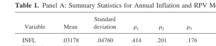
Table 1 reports the means, standard deviations, autocorrelations, and Phillips–Perron unit root test statistics for these various measures of RPV as well as for inflation. All of
6Given the definition in (1), a more descriptive name for the concept involved would be the variability of relative price changes. However, the name “relative price variability” and the acronym RPV are so entrenched in the literature that I continue to use them.
the measures of RPV and inflation exhibit significant autocorrelations for one or more periods. However, all these series are found to be stationary and can be reasonably used in the regressions below. Phillips–Perron unit root tests reject the hypothesis of a unit root in each of the series at the 5% level.
Panel A of Table 2 reports the results of regressions of the three annual measures of RPV upon the square of annual inflation and a constant. The coefficient estimate on the square of inflation is positive and significant at the 1% level in each of the regressions. The square of inflation, rather than inflation, is used as an explanatory variable in accordance with previous studies that test the prediction that RPV will be associated with the absolute magnitude of inflation. However, deflationary episodes are so rare in the US after WWII that it makes little difference whether inflation or the square of inflation is used as an explanatory variable. Panel B of Table 2 reports the results of regressions of the three monthly measures of RPV upon the square of monthly inflation and a constant. Again, the coefficient estimate on the square of inflation is positive and significant at the 1% level in each of the regressions.
So long as firm profits are increasing in output prices and decreasing in input prices, it immediately follows that the variability of profits will increase with RPV. Whether expected firm profits are directly affected in any way by RPV is more controversial. In partial-equilibrium models, the answer depends upon the ability of firms to adjust production decisions when the relative price changes occur. If production decisions cannot be altered, then expected profits will not affected by RPV. If production decisions can be altered, then expected profits will increase with RPV due to the convexity of the profit function. In the model of section III, I assume that firms cannot adjust production decisions to take advantage of relative price changes. This focuses attention on the indirect effect of RPV on agency costs via its effect on the variability of profits.
Table 1. Panel A: Summary Statistics for Annual Inflation and RPV Measures, 1947–1996
Variable Mean
Standard
deviation r1 r2 r3 r4
Phillips-Perron test statistic
INFL .03178 .04760 .414 .201 .176 .135 24.37
RPV14A .00140 .00246 .561 .086 2.016 .016 23.54
RPV64A .00445 .00508 .506 .188 .082 2.016 23.88
RPV148A .00579 .00525 .502 .207 .029 2.052 23.90
INFL is (annual) inflation and RPV14A, RPV64A, and RPV148A are annual measures of relative price variability. The column forrireports the autocorrelation at lag i. The final column reports the Phillips-Perron test statistic for a unit root in the level of the variable in question. In each case, the 5% critical value for rejection of the null hypothesis of a unit root is22.92.
Panel B: Summary Statistics for Monthly Inflation and RPV Measures, 1947.01–1997.10
Variable Mean
Standard
deviation r1 r3 r6 r12
Phillips-Perron test statistic
INFL .00271 .00697 .357 .266 .245 .196 217.80
RPV14M .00012 .00022 .332 .199 .223 .130 218.24
RPV64M .00062 .00083 .457 .303 .219 .164 215.67
RPV148M .00086 .00093 .629 .387 .311 .290 211.74
III. The Model
Assumptions
The representative firm is composed of a manager and a bloc of risk-neutral outside shareholders who hold only equity claims. The real profits of the firm before the manager is paid are y5u1e where e[[emin,`) is the level of “effort” chosen by the manager and u is a random disturbance to real profits due to changes in relative prices.8 The disturbanceuis normally distributed with mean zero, variancesu2
, and is independent of
e as well as the disturbances experienced by other firms.9 The firm must commit to production beforeuis realized so the firm cannot react to any relative price changes.
The shareholders observe y, but neither u nor e individually. Shareholders cannot directly observe the various relative price changes that affect profits, nor can they directly observe managerial actions. The assumption that effort is unobservable reflects the fact that, even if it were feasible for shareholders to observe the managerial actions directly, it would be difficult for them to judge whether managerial actions were appropriate. The job of a manager is entrepreneurial rather than repetitive.
8“Effort” refers to not only effort in the literal sense, but also other managerial actions that affect profits such as empire-building, the pursuit of projects designed to enhance the reputation of the manager rather than profits, and other forms of perquisites consumption.
9One extension of the model would be to allow the shareholders of the firm to observe the average profits in the firm’s industry. This would help them more accurately assess the level of effort chosen by the manager. However, the qualitative results of the model would still hold unlessucan be determined exactly by observing industry performance.
Table 2. Panel A: Estimation Results for RPVt5b01b1(INFLt) 21
etUsing Annual Data
Dependent variable Constant (INFLt)2 R2
RPV14At .000133*** .425*** .97
INFL is (annual) inflation and RPV14A, RPV64A, and RPV148A are annual measures of relative price variability. The standard errors of the coefficient estimates are reported in parentheses. All standard errors are calculated according to the procedure suggested in White (1980) to allow for residuals that are heteroskedastic; *** indicates significance at the 10% level.
Panel B: Estimation Results for RPVt5b01b1(INFLt) 21
The manager and the shareholders must choose a managerial compensation contract that is linear in profits: w5a1by. For purposes of exposition, the profit incentives of
the manager are assumed to take the form of an explicit link between profits and salary rather than the form of required managerial equity holdings. Requiring that the wage contract be linear in profits is a restrictive assumption, but many real-world incentive contracts are actually linear in output or profits. One advantage that linear schemes possess is that they are easy to administer and explain. Also, more complex nonlinear incentive schemes are more fragile in the sense that if the conditions for which they were designed change, they may provide very inappropriate motivation.
The utility function of the manager is UM(W) 5 2exp
2rW
where r. 0 and the net wealth W of the manager is money income w from the firm less his dollar cost C(e) of expending effort. The cost-of-effort function satisfies C(emin)50 with lime3`C9(e)5 `,
C9(e). 0, and C0(e).0. The manager has employment opportunities outside the firm that would provide a sure wage of w# with no expenditure of effort.
The optimization problem of the manager takes a very simple form because of the combination of normally distributed profits, a wage contract which is linear in profits, and an exponential utility function. Under these assumptions, the random wage w coupled with effort e is equivalent in utility to a certain income (certainty equivalent) of
CEM~w, e!5E@w#2
r
2Var@w#2C~e! (2)
where E[ ] and Var[ ] are the expectation and variance operators, respectively.10 The outside shareholders care only about wealth and are risk-neutral with respect to income from the firm. Individual shareholders ultimately may well be risk-averse like the manager, but they (unlike the manager) can diversify across firms with independentu’s. Because the outside shareholders receive y less whatever monetary payment is made to the manager, the certainty equivalent of the shareholders is:
CES@y2w#5E@y2w#. (3)
Results
Once the managerial compensation contract is signed, the utility of the manager is maximized by exerting a level of effort that equates his marginal costs of exerting effort with his marginal benefits of exerting effort. This results in a choice of effort that satisfies:
C9~e!5b. (4)
The assumption C0(e).0 implies that the solution to Eq. (4) is unique and satisfies the second-order sufficient condition for a maximum. It also implies that effort increases step-for-step with incentives.
From the shareholders’ perspective, a compromise must be struck between the mar-ginal benefits of b, namely higher expected profits, and the marginal costs of b, the additional base pay that must be paid to attract the manager because of his disutility of bearing risk. The shareholders will offer a contract {a, b} to the manager which maximizes their certainty equivalent (3) subject to the constraints that the incentive
compatibility constraint (4) is satisfied, and that the certainty equivalent of the manager given by Eq. (2) equals w# so that manager is just induced to accept the contract. Substituting the constraints yields the following optimization problem for the sharehold-ers:
After solving Eq. (5) for e (and, implicitly, for b), the base wage is simply set at the minimum needed to attract the manager to the job.
The maximization problem of the shareholders has the first-order condition:
12rC9~e!C0~e!su
2
2C9~e!50. (6)
The second-order sufficient condition for the solution of (6) to be a maximum is that:
c~e!52C0~e!2rsu2@C0~e!C0~e!1C9~e!C-~e!#,0. (7)
Let e* represent the optimal level of effort andb* represent the corresponding optimal level of managerial profit incentives. Total differentiation of Eq. (6) yields:
e*
su25
rC9~e*!C0~e*!
c~e*! . (8)
If the second-order sufficient condition for a maximum holds so that the denominator of Eq. (8) is negative, then the assumptions C9(e).0 and C0(e).0 imply that the optimal level of effort decreases the variance of profits. It immediately follows that the optimal level of incentives decreases with the variance of profits, because higher effort can only be induced by higher incentives. This sort of prediction of models of the shareholder-manager relationship regarding the relationship between incentives and the variance of profits is well known, and has been investigated empirically. Spremann (1987) and Garen (1994), for instance, obtain a similar prediction using the additional assumption that the cost-of-effort function is quadratic so that a closed-form solution for the optimal level of incentives can be obtained. Furthermore, both Garen and Aggarwal and Samwick (1999) have tested this prediction using US data and have found evidence that the strength of a firm’s managerial profit incentives does decrease with the variability of its equity returns. By contrast, the predictions of models of the shareholder-manager relationship regard-ing the relationship between the level of expected profits and the variance of profits have not received much attention in the literature. The first such prediction obtained from the model of this paper is that the real profits of the firm before the manager is paid ( y5u1 e) will decrease with the variance of profits. This is immediate because effort decreases
with the variance of profits. The second, and more important, prediction is that the expected real profits accruing to the shareholders also will decrease with the variance of profits. From Eq. (5), these are:
f~e*; r, su2, w#!
This is always negative becauseb* and r are positive.
The result in Eq. (10) means that a marginal increase in the variance of profits in the amount ofDsu2causes a marginal loss of .5r(b*)2(Dsu2) to the shareholders of the firm.11
The origin of this loss is that the manager dislikes risk, and suffers a disutility of .5r(b*)2(Dsu2) from bearing his share (b*) of the extra variance in profits. Because
shareholders set the base pay of the manager just high enough to meet his reservation utility, the shareholders must increase the base pay of the manager by .5r(b*)2(Dsu2) to
retain the manager. Thus, the manager continues to receive his reservation utility while the shareholders, the residual claimants, suffer a decrease in expected real profits of .5r(b*)2(Dsu2).
The result in Eq. (10) also means that the marginal loss to shareholders due to an increase in the variance of profits increases withb*. Intuitively, this is because, all else equal, firms with strong existing managerial profit incentives have more to lose on the margin. Consider the extreme case of a firm with which gives its manager no profit incentives whatsoever. In such a case, the shareholders are indifferent to an increase in the variance of profits because the manager does not bear any more risk and therefore does not need to be compensated for doing so. The shareholders are indifferent because they have already acquiesced in very high agency costs and have nothing left to lose, in essence.
IV. Empirical Tests
Two predictions emerge directly from Eq. (10). First, an increase in the variance of profits will cause a decrease in expected profits for firms. Second, an increase in the variance of profits will cause greater decreases in expected profits for firms with strong managerial profit incentives than for firms with weak managerial profit incentives. While these predictions are testable with the proper accounting data, I test instead the implications for real equity returns. If stock markets are efficient and the variability of profits increases with RPV, then Eq. (10) implies that (1) real equity returns will fall when bad news is received regarding the amount of RPV that firms will confront, and that (2) the severity of the negative relationship between real equity returns and bad news about RPV will increase with the strength of managerial profit incentives.
These predictions are tested by examining and contrasting the behavior of real equity returns across the ten size-decile portfolios of firms listed on the New York Stock Exchange (NYSE). These portfolios range from the largest 10% in terms of market-capitalization to the smallest 10% in term of market-market-capitalization.12 The focus upon portfolios of firms grouped by market-capitalization is chosen because there is substantial
11This is true whether or not managerial incentives can be adjusted in response to the marginal increase in the variability in profits. If incentives cannot be adjusted, then .5r(b*)2(Ds
u
2) is the exact amount of the loss. If incentives can be adjusted, then .5r(b*)2(Ds
u
2) is an arbitrarily close approximation to the loss. Only for large increases in the variability of profits will the loss to the shareholders be noticeably ameliorated (though not eliminated) through the weakening of managerial incentives.
evidence that the strength of managerial incentives decreases with firm size. Drawing on data from the 1940s through the 1980s, Lewellen (1971), Demsetz (1983), and Jensen and Murphy (1990) all find that the percentage of stock held by CEOs and other top managers decreases with firm size. Jensen and Murphy, for instance, find that the median CEO shareholding in the smallest 50% of the firms in their sample is three times as high as the median CEO shareholding in the largest 50% of the firms (.49% vs. .14%). Jensen and Murphy also find that other forms of managerial incentives such as bonuses and salary increases tied to firm performance are stronger for CEOs in smaller firms.13
The empirical exercises below proceed in three steps. Step one verifies the widely observed negative correlation between inflation in period t and real equity returns in period t. Step two verifies the results of Fama (1981) and Kaul (1987) by adding a measure of real output growth in period t 1 1 as an additional explanatory variable to the regressions of step one. While imperfect, this is the proxy used in the studies of Fama and Kaul for news received in period t regarding future real output growth.14 Step three examines the results of adding the change in RPV between period t 2 1 and t as an additional explanatory variable to the regressions of step two. While also admittedly imperfect, this is a proxy for the news received in period t about the amount of RPV that will confront firms in period t and beyond.
Finally, although many studies of stock returns and inflation decompose inflation into expected and unexpected components, actual inflation is used as the single inflation variable here. This is done because the additional insight gained by decomposing inflation into expected and unexpected components is small, and does not justify the econometric problems created. Decomposing inflation provides little additional insight because the various theories proposed to explain the relationship between inflation and real equity returns do not make sharply distinct predictions regarding the expected and unexpected components of inflation. By contrast, the econometric problems involved are substantial. In particular, the common procedure in this literature of generating measures of expected and unexpected inflation with a preliminary model of inflation, and then using those as explanatory variables in a second regression creates an errors-in-variables problem.15
Data
The data are annual US data from 1947 to 1997. Annual inflation (INFL) and annual RPV are measured using PPI data as described in section II. For brevity, only a single measure of annual RPV, namely RPV14A, is employed in the regressions below. The results using other measures of RPV are similar. The change in RPV in year t is denoted as DRPV14A and is defined as the difference between RPV14A in years t and t 21.
returns is more pronounced among the more cyclical industries. Because managerial incentives appear to vary in a simple and systematic way with firm size, I group firms by size rather than industry.
13Incidentally, this pattern matches the prediction of the model of this paper regarding the optimal level of managerial incentives. Larger firms tend to have more absolute risk in profits and therefore should tend to have weaker managerial incentives.
14Ideally, a direct measure of the change in beliefs during year t regarding future real output growth would be used as the additional regressor to test the proxy hypothesis. However, given the difficulty of assessing changes in beliefs, I follow Fama and Kaul in the use of actual real output growth in year t11 as a proxy for such changes.
Annual data on nominal equity returns for each of the ten size-decile portfolios of NYSE stocks is taken from Ibbotson Associates (1998).16Real equity returns for the ith size-decile portfolio (RRETi) are computed by subtracting inflation (INFL) from the nominal equity returns of the ith size-decile portfolio. The measure of real activity used is GDP in 1992 chain-weighted dollars from the US National Income and Product Accounts (NIPA).17Growth in real GDP in year t is measured as the difference in the logs of real GDP in years t and t21. The results below are essentially unchanged if the index of industrial production is used as the measure of real activity instead of real GDP.
Table 3 reports the means, standard deviations, autocorrelations, and Phillips-Perron unit root test statistics for RRET1 through RRET10 as well as for INFL, DGDP, and DRPV14A over the sample period. All of the series are stationary. Phillips-Perron unit root tests reject the hypothesis of a unit root in each of the series at the 1% level.
Related Work
Kaul and Seyhun (1990) perform empirical work somewhat similar to that outlined above. They too examine the hypothesis that the RPV that tends to accompany inflation may have adverse economic effects and may account for some of the negative correlation between inflation and real equity returns. The primary difference between the present study and that of Kaul and Seyhun is the number of predictions that are made and tested. Kaul and Seyhun, on the basis of a brief discussion of possible reasons why RPV might have adverse economic effects, test only the prediction that increases in RPV will have an
16The equity return data reported in Ibbotson Associates (1998) for the ten size-decile portfolios of NYSE stocks is compiled by the Center for Research in Security Prices.
17These data were taken from the Economic Information Service (EIS) which reformats NIPA data into spreadsheet form. The website of EIS is http://www.econ-line.com.
Table 3. Summary Statistics for Annual Variables, 1947–1997
Variable Mean
Standard
deviation r1 r2 r3 r4
Phillips-Perron test statistic
INFL .030788 .047632 .408 .198 .174 .143 24.35
DRPV14A 2.000012 .003243 2.145 2.278 2.130 2.164 28.68
DGDP .032511 .024830 .014 2.088 2.106 .011 26.77
RRET1 .103660 .181151 2.035 2.119 .140 .289 26.95
RRET2 .114346 .190206 2.068 2.211 .117 .314 27.33
RRET3 .125322 .201030 2.108 2.271 .054 .283 27.85
RRET4 .127602 .215838 2.099 2.333 .041 .295 27.89
RRET5 .125285 .218155 2.029 2.255 .061 .239 27.13
RRET6 .134142 .236495 2.067 2.299 .019 .212 27.52
RRET7 .136802 .250597 2.047 2.298 .021 .216 27.30
RRET8 .143102 .267294 2.021 2.319 .031 .180 27.14
RRET9 .139272 .277327 2.010 2.277 2.007 .179 26.99
RRET10 .141112 .310634 .007 2.358 .069 .185 26.92
adverse effect on equity returns.18On the basis of the model of section III, by contrast, the present study tests that prediction as well as the cross-sectional prediction that small firms will be more affected by news about RPV than will large firms. One consequence of this difference is that the present study examines the behavior of NYSE stocks grouped into ten size-deciles, while the empirical work of Kaul and Seyhun examines only the behavior of the market portfolio of NYSE stocks. A second important difference between the present study and that of Kaul and Seyhun is that they attempt the problematic task of decomposing inflation into expected and expected components.
Their findings are as follows. First, when real equity returns are regressed only on expected and unexpected inflation, the coefficient estimates on both components of inflation are negative and significant at the 10% level. Second, when real equity returns are regressed on a measure of RPV as well as upon expected and unexpected inflation, the measure of RPV attracts a coefficient estimate which is negative and significant at the 5% level, while the coefficient estimates on expected and unexpected inflation are reduced in size and become insignificant.19Finally, when a measure of growth in future real output growth is added as a fourth regressor, the size and significance of the coefficient estimates
18Kaul and Seyhun cite two specific channels by which RPV might have adverse economic effects. The first is an increase in RPV might reduce the information content of relative prices. The second is that an increase in RPV might lead to the implementation of more costly institutional arrangements such as more frequent contracting.
19Kaul and Seyhun use PPI data, as I do, to construct a measure of RPV.
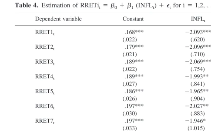
Table 4. Estimation of RRETii5b01b1(INFLt)1etfor i51,2, . . . 10 Using Annual Data
Dependent variable Constant INFLt R2
RRET1t .168*** 22.093*** .30
(.022) (.620)
RRET2t .179*** 22.096*** .27
(.021) (.710)
RRET3t .189*** 22.069*** .24
(.022) (.754)
RRET4t .189*** 21.993** .19
(.027) (.841)
RRET5t .186*** 21.965** .18
(.026) (.904)
RRET6t .197*** 22.027** .17
(.030) (.883)
RRET7t .197*** 21.946* .14
(.033) (1.015)
RRET8t .201** 21.876* .11
(.037) (1.061)
RRET9t .205*** 22.125* .13
(.038) (1.095)
RRET10t .200*** 21.915 .09
(.043) (1.220)
on expected and unexpected inflation are further reduced, while the coefficient estimate on RPV remains negative and significant at the 5% level.
Results
Regressions of real equity returns in period t upon contemporaneous inflation and a constant yield the traditional results. The coefficient estimates on inflation are negative for all ten of the size-decile portfolios of NYSE stocks, and are significantly different from zero at the 10% level for all of the portfolios except the one composed of the smallest firms. Table 4 reports the estimation results. Note that RRET1 denotes the real equity returns of the portfolio composed of the largest firms, while RRET10 denotes the real equity returns of the portfolio composed of the smallest firms.
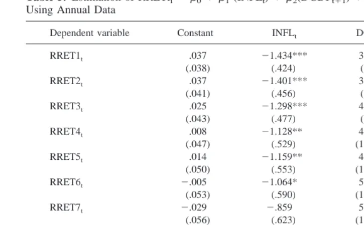
The addition of a measure of future real output growth (DGDPt11) as an explanatory variable to the battery of regressions reported in Table 4 also yields the traditional results. For each of the ten portfolios, a positive coefficient estimate on future real output growth is obtained while simultaneously the size and significance of the negative coefficient estimate on inflation is reduced. Table 5 reports the estimation results.
The coefficient estimates on future real output growth are positive and significant at the 1% level for each of the ten portfolios. At the same time, the coefficient estimates on inflation, while negative in every case, are not significantly different from zero for portfolios 7–10 at any level of significance, and are significantly different from zero at the 1% level of significance only for portfolios 1–3. Both of these findings support the proxy
Table 5. Estimation of RRETii5b01b1(INFLt)1b2(DGDPt11)1etfor i51,2, . . . 10 Using Annual Data
Dependent variable Constant INFLt DGDPt11 R2
RRET1t .037 21.434*** 3.315*** .48
(.038) (.424) (.805)
RRET2t .037 21.401*** 3.634*** .47
(.041) (.456) (.866)
RRET3t .025 21.298*** 4.271*** .48
(.043) (.477) (.907)
RRET4t .008 21.128** 4.696*** .45
(.047) (.529) (1.004)
RRET5t .014 21.159** 4.490*** .41
(.050) (.553) (1.051)
RRET6t 2.005 21.064* 5.208*** .43
(.053) (.590) (1.120)
RRET7t 2.029 2.859 5.842*** .43
(.056) (.623) (1.183)
RRET8t 2.043 2.720 6.35*** .42
(.061) (.674) (1.281)
RRET9t 2.042 2.947 6.376*** .42
(.063) (.697) (1.324)
RRET10t 2.091 2.569 7.704*** .42
(.070) (.784) (1.489)
hypothesis as a partial explanation of the puzzling negative correlation between inflation and real equity returns. However, the fact that many of the coefficient estimates on inflation remain negative and significant at traditional levels indicates that the proxy hypothesis does not fully explain the negative correlation between inflation and real equity returns.
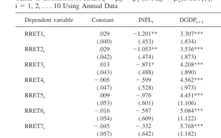
Finally, a measure of the change in relative price variability between period t21 and period t (DRPV14At) is added as an explanatory variable to the battery of regressions
reported in Table 5. As noted above, DRPV14Atis a proxy for the news received in period
t about the amount of RPV that will confront firms in period t and beyond. Table 6 reports
the results of portfolio-by-portfolio regressions of real stock returns on INFLt, DGDPt11, DRPV14At, and a constant. Table 7 reports the results of joint estimation for all ten
portfolios using the seemingly unrelated regression (SUR) method to take advantage of any information provided by correlations between the error terms.
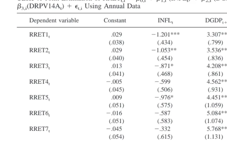
Several patterns are evident in Tables 6 and 7. First, the coefficient estimates on DGDPt11 are positive and significant at the 1% level for each of the ten portfolios. Second, the bulk (8 of 10 in both separate and joint estimation) of the coefficient estimates on DRPV14At are negative and significant at the 5% level. The exceptions, in both
separate and joint estimation, occur for the first and the fifth size-decile portfolios where the coefficient estimates on DRPV14At, while negative, are not significant at traditional
levels.
Third, the coefficient estimates on DRPV14At tend to be more negative for the
portfolios composed of small firms than for those composed of large firms. Formally, a
Table 6. Estimation of RRETii5b01b1(INFLt)1b2(DGDPt11)1b3(DRPV14At)1etfor i51, 2, . . . 10 Using Annual Data
Dependent variable Constant INFLt DGDPt11 DRPV14At R2
RRET1t .029 21.201** 3.307*** 29.130 .50
Wald test of the hypothesis that the coefficients on DRPV14Atare equal for portfolios 1
and 10 (the largest firms and the smallest firms) under joint estimation yields a Chi-square (1) statistic of 2.26 which has a p-value of .13. A Wald test of the hypothesis that the coefficients on DRPV14Atare equal for portfolios 1, 2, 9, and 10 under joint estimation
yields a Chi-square (3) statistic of 7.37 which has a p-value of .06.20
Fourth, the inclusion of DRPV14Atas an additional explanatory variable reduces the
size and significance of the coefficient estimates on inflation for each of the ten portfolios. This can be seen from a comparison of Tables 5 and 6 or Tables 5 and 7. The inclusion of DRPV14Atas an additional explanatory variable renders the coefficient estimates on
inflation insignificant at the 5% level for all of the portfolios except for the first and second in both separate and joint estimation.
In brief, the result are as follows. First, real equity returns appear to react negatively to bad news regarding RPV. Second, there is some evidence that the severity of the negative relationship between real equity returns and bad news about RPV increases with firm size. Finally, the results suggest that the agency cost hypothesis complements the proxy hypothesis by explaining much of the negative relationship between inflation and real equity returns that persists after controlling for output growth.
20Similar tests of the equality of the coefficients on DRPV14A
tfor the sets of portfolios {1, 2, 3, 8, 9, 10}
and {1, 2, 3, 4, 7, 8, 9, 10} yield, respectively, a Chi-square (5) statistic of 7.82 with a p-value of .17, and a Chi-square (7) statistic of 15.36 with a p-value of .03.
Table 7. Joint Estimation of RRETt,i5b0,i1b1,i(INFLt)1b2,i(DGDPt11)1
b3,i(DRPV14At)1et,iUsing Annual Data
Dependent variable Constant INFLt DGDPt11 DRPV14At
RRET1t .029 21.201*** 3.307*** 29.130
(.038) (.434) (.799) (6.036)
RRET2t .029 21.053** 3.536*** 214.518**
(.040) (.454) (.836) (6.318)
RRET10t 2.113 .039 7.700*** 223.619**
(.069) (.783) (1.442) (10.901)
V. Conclusion
According to the proxy hypothesis of Fama (1981), the puzzling negative correlation between inflation and real equity returns is simply induced by the opposite effects that news about future real output growth has upon equity prices and the price level. This hypothesis has received substantial support. Empirical studies of real equity returns that control for news about future real output growth generally find a reduction in the size and significance of the coefficient estimates on both the expected and unexpected components of inflation. However, the coefficient estimates on the inflation variables, particularly that of the unexpected component of inflation, often remain negative and significant at traditional levels of significance.
In this paper, I hypothesize that agency costs may account for the negative relationship between inflation and real equity returns that persists after controlling for news about future real output growth. This is suggested by the empirical evidence that relative price variability (RPV) increases with inflation and by the prediction of a simple principal-agent model that the agency costs borne by firms will increase with the variability of profits (which presumably increase with RPV). Support for the hypothesis is found in regressions of real equity returns upon inflation, a measure of news about future real output growth, and a measure of news about RPV. In this specification, the coefficient estimates on news about RPV are consistently negative while the coefficient estimates on inflation are generally insignificant.
I would like to thank Chris Jones, Bill Lastrapes, Ronald McKinnon, Julie Schaffner, Ron Warren, David VanHoose (the editor), Kenneth Kopecky (the executive editor), and several anonymous referees for their helpful comments. Any remaining errors are mine.
References
Aggarwal, R. K., and Samwick, A. A. Feb. 1999. The other side of the trade-off: the impact of risk on executive compensation. Journal of Political Economy 107(1):65–105.
Amihud, Y. Feb. 1996. Unexpected inflation and stock returns revisited—evidence from Israel.
Journal of Money, Credit, and Banking 28(1):22–33.
Bodie, Z. May 1976. Common stocks as a hedge against inflation. Journal of Finance 31(2):459– 470.
Boudoukh, J., and Richardson, M. Dec. 1993. Stock returns and inflation: a long-horizon perspec-tive. American Economic Review 83(5):1346–1355.
Boudoukh, J., Richardson, M., and Whitelaw, R. F. Dec. 1994. Industry returns and the fisher effect.
Journal of Finance 49(5):1595–1615.
Boyle, G. W., and Young, L. Mar. 1988. Asset prices, commodity prices, and money: a general equilibrium, rational expectations model. American Economic Review 78(1):24–45.
Danthine, J.-P., and Donaldson, J. B. May 1986. Inflation and asset prices in an exchange economy.
Econometrica 54(3):585–605.
Debelle, G., and Lamont, O. Feb. 1997. Relative price variability and inflation: evidence from U.S. cities. Journal of Political Economy 105(1):132–152.
Demsetz, H. June 1983. The structure of ownership and the theory of the firm. Journal of Law and
Fama, E. Sept. 1981. Stock returns, real activity, inflation, and money. American Economic Review 71(4):545–565.
Fama, E., and Schwert, G. W. Nov. 1977. Asset returns and inflation. Journal of Financial
Economics 5(2):115–146.
Feldstein, M. Dec. 1980. Inflation and the stock market. American Economic Review 70(5):839– 847.
Firth, M. June 1979. The relationship between stock market returns and inflation. Journal of
Finance 34(3):743–749.
Fischer, S. May–June 1982. Relative price variability and inflation in the United States and Germany. European Economic Review 18(1/2):171–196.
Freund, R. J. July 1956. The introduction of risk into a programming model. Econometrica 24(3):253–263.
Friend, I., and Hasbrouck, J. 1982. The effect of inflation on the profitability and valuation of U.S. corporations. In Saving, Investment, and Capital Markets in an Inflationary Economy (M. Sarnat, and G. P. Szego¨, eds.). Cambridge, MA: Ballinger, pp. 37–119.
Garen, J. E. Dec. 1994. Executive compensation and principal-agent theory. Journal of Political
Economy 102(6):1175–1199.
Geske, R., and Roll, R. Mar. 1983. The fiscal and monetary linkage between stock returns and inflation. Journal of Finance 38(1):1–33.
Grier, K. B., and Perry, M. J. Oct. 1996. Inflation, inflation uncertainty, and relative price dispersion: evidence from bivariate GARCH-M models. Journal of Monetary Economics 38(2): 391–405.
Gultekin, N. B. Mar. 1983. Stock market returns and inflation: evidence from other countries.
Journal of Finance 38(1):49–65.
Ibbotson Associates. 1998. Stocks, Bonds, Bills, and Inflation 1998 Yearbook. Chicago: Ibbotson Associates.
Jaffe, J. F., and Mandelker, G. May 1976. The “Fisher effect” for risky assets: an empirical investigation. Journal of Finance 31(2):447–458.
Jensen, M. C., and Murphy, K. J. Apr. 1990. Performance pay and top-management incentives.
Journal of Political Economy 98(2):225–264.
Kaul, G. June 1987. Stock returns and inflation. Journal of Financial Economics 18(2):253–276. Kaul, G., and Seyhun, H. N. June 1990. Relative price variability, real shocks, and the stock market.
Journal of Finance 45(2):479–496.
Lewellen, W. G. 1971. The Ownership Income of Management. New York: National Bureau of Economic Research.
Marshall, D. A. Sept. 1992. Inflation and asset returns in a monetary economy. Journal of Finance 47(4):1315–1342.
McDevitt, C. L. July 1989. The role of the nominal tax system in the common stock returns/expected inflation relationship. Journal of Monetary Economics 24(1):93–107.
Mills, F. C. 1927. The Behavior of Prices. New York: National Bureau of Economic Research. Modigliani, F., and Cohn, R. A. 1982. Inflation, rational valuation and the market. In Saving,
Investment, and Capital Markets in an Inflationary Economy (M. Sarnat, and G. P. Szego¨, eds.).
Cambridge, MA: Ballinger, pp. 121–166.
Nelson, C. R. May 1976. Inflation and rates of return on common stock. Journal of Finance 31(2):471–483.
Newey, W. K., and West, K. D. May 1987. A simple, positive semi-definite, heteroskedasticity and autocorrelation consistent covariance matrix. Econometrica 55(3):703–708.
Pagan, A. Feb. 1984. Econometric issues in the analysis of regressions with generated regressors.
Parks, R. Feb. 1978. Inflation and relative price variability. Journal of Political Economy 86(1): 79–95.
Parsley, D. C. Aug. 1996. Inflation and relative price variability in the short and long run: new evidence from the United States. Journal of Money, Credit, and Banking 28(3, pt. 1):323–341. Spremann, K. 1987. Agent and principal. In Agency Theory, Information, and Incentives (G.
Bamberg, and K. Spremann, eds.). Berlin: Springer-Verlag, pp. 3–37.
Vanderhoff, J., and Vanderhoff, M. Dec. 1986. Inflation and stock returns: an industry analysis.
Journal of Economics and Business 38(4):341–352.
Wei, K. C. J., and Wong, K. M. Feb. 1992. Tests of inflation and industry portfolio returns. Journal
of Economics and Business 44(1):77–94.