ESTIMATING AIRCRAFT HEADING
BASED ON LASERSCANNER DERIVED POINT CLOUDS
Z. Koppanyia,b, *, C. K. Toth a
a Dept. of Civil, Environmental and Geodetic Engineering, The Ohio State University, 470 Hitchcock Hall, 2070 Neil Ave., Columbus, OH 43210 - (koppanyi.1, toth.2)@osu.edu
b Dept. of Photogrammetry and Geoinformatics, Budapest University of Technology and Economics, 3 Műegyetem rkp. Budapest, H-1111, Hungary – [email protected], [email protected]
Commission I, WG I/2
KEY WORDS: Pose estimation, Iterative Closest Point, entropy minimization, laser profile scanners, aviation safety
ABSTRACT:
Using LiDAR sensors for tracking and monitoring an operating aircraft is a new application. In this paper, we present data processing methods to estimate the heading of a taxiing aircraft using laser point clouds. During the data acquisition, a Velodyne HDL-32E laser scanner tracked a moving Cessna 172 airplane. The point clouds captured at different times were used for heading estimation. After addressing the problem and specifying the equation of motion to reconstruct the aircraft point cloud from the consecutive scans, three methods are investigated here. The first requires a reference model to estimate the relative angle from the captured data by fitting different cross-sections (horizontal profiles). In the second approach, iterative closest point (ICP) method is used between the consecutive point clouds to determine the horizontal translation of the captured aircraft body. Regarding the ICP, three different versions were compared, namely, the ordinary 3D, 3-DoF 3D and 2-DoF 3D ICP. It was found that 2-DoF 3D ICP provides the best performance. Finally, the last algorithm searches for the unknown heading and velocity parameters by minimizing the volume of the reconstructed plane. The three methods were compared using three test datatypes which are distinguished by object-sensor distance, heading and velocity. We found that the ICP algorithm fails at long distances and when the aircraft motion direction perpendicular to the scan plane, but the first and the third methods give robust and accurate results at 40m object distance and at ~12 knots for a small Cessna airplane.
1. INTRODUCTION
Monitoring aircraft parameters, such as position and heading, during take-off, landing and taxiing can improve airport safety, as modeling the trajectory helps understand and assess the risk of the pilot’s driving patterns on the runways and taxiways (e.g. centerline deviation, wingspan separation). This information can be used in aircraft and airport planning; e.g., whether the airport meets the standardized criteria or providing data for modification of airport standards and pilot education (Wilding et al., 2011).
Extracting this information requires sensors which are able to capture these parameters. The on-the-board GPS/GNSS and IMU sensors could provide such data, but it is hard to assess, as these systems provide no interface and then due to varying aircraft specification, privacy and other issues. The radar systems, such as those applied by ILS (Instrument Landing System) are primarily used for aiding pilots and not for accurately tracking aircraft on the ground. Furthermore, the general safety, tracking and maintenance sensors, deployed at airports, usually cannot collect real-time 3D data from operating aircrafts. For this reason, other sensor types should be considered and, consequently, to be investigated.
To study taxiing behavior, Chou et al. used positioning gauges to obtain data at the Chiang-Kai-Shek International Airport (Chou, 2006). The gauges recorded the passing aircraft’s nose gear on the taxiway. Another study from FAA/Boeing investigated the 747s’ centerline deviations at JFK and ANC airports (Scholz, 2003a and 2003b). They used laser diodes at two locations to
measure the location of the nose and main gears. Another report deals with wingspan collision using the same sensors (Scholz, 2005). The sensors applied and investigated by these studies allow only point type data acquisition (light bar).
LiDAR (Light Detection and Ranging) is a suitable remote sensing technology for this type of data acquisition, as it directly captures 3D data and is fast. In this study, we test profile laserscanners for aircraft body heading estimation; note that heading is an important parameter for estimating centerline deviation or for determining taxiing patterns. Although this study focuses on the heading estimation, with minor extensions, the presented methods are also able to obtain position and other navigation information from the measurements. This effort is a pioneer work, as no study or investigation has been conducted in connection with aircraft heading estimation using LiDAR profile sensors.
2. PROBLEM DEFINITION
Different types of laser sensors are able to produce various type of point clouds depending on the sensor’s resolution, range, field of view, etc. In this study, a 360º FOV Velodyne HDL-32E laser scanner with an angular resolution of 0.6º is used (http://velodyne.com). The scanner’s 32 sensors, arranged perpendicular to the main plane provide a FOV of +10 - -30º with 1.33º separation. This sensor is very popular in autonomous robotics systems. The choice of the sensor was highly influenced by its relatively low cost.
Regarding the sensor arrangement, the horizontal installation is generally better for localization; for example, Huijing et al. presents a system for tracking pedestrians in a dense area (Huijing, 2005) and (Weiss, 2007) shows a navigation application. The vertical placement of the sensor is the typical mapping arrangement to support 3D model reconstruction. Rosell presents a method, where a horizontally placed sensor attached to the vehicle scanned tree orchards and the 3D model was reconstructed from the profiles. In the current study, the same 2D reconstruction method is applied; the 2D scanner will be placed next to the runway and taxiway and the 3D model will be created fusing the consecutive profiles. But, in contrast to the previous studies, where the sensor is moving, the scanner is fixed at certain positions and scans the aircraft’s move. The train profile validation system (PVS) from the Signal and System Technik Company uses a similar idea to validate train profiles to
prevent damages and accidents
(http://www.sst.ag/en/products/diagnostic-systems/profile-validation-system-pvs/). Their system consists of a gate frame structure with laser scanners around the train cross-section. When the train passes under the gate, the sensors scan the vehicle, and the software creates a full 3D model. Note the train motion is confined to the track, so the reconstruction problem is simple.
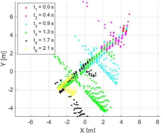
Comparing our task to mobile laser scanning (MLS), the key differences can be easily identified. First, in our case the object is moving, not the platform, and secondly, the goal is not the mapping of the entire environment, just observing and tracking a moving object and deriving some navigation parameters. In MLS studies, the segmentation of the scene generally poses big challenges, while in our case it is relatively simple, because the runaway area is easily determined/mapped from the static platform. Sample point clouds of a moving aircraft captured by the vertically installed Velodyne sensor at different times are shown in Figure 1.
Figure 1. Scans of an aircraft, taken at different epochs (top view)
These point clouds are the input for the algorithms to extract navigation information. In the subsequent discussion, the heading and velocity are assumed to be constant between the entering and leaving points of the scanned area. These assumptions are realistic, as the vehicle is moving relatively fast, thus it is not able to change its orientation in the short range covered by the sensor.
At this point, we give the motion equations along the X and Y axes, for distance traveled, ∆ and ∆ , respectively, between two consecutive scans, as the function of heading and velocity, assuming constant independent variables:
∆ = � ∗ ∆ = cos � ∗ � ∗ ∆ (1)
where ∆ is the time difference between two scans,
� is the unknown constant heading in the sensor coordinate system,
� is the unknown constant speed of the aircraft,
� , � are the and components of this velocity.
This system is determined due to the fact of two unknowns belong to two equations. The examination of the error propagation of the Eq. 1 is important to estimate the accuracy level that has to be achieved to reach the required accuracy of the parameters (�, �). The derived error propagation equation, see Appendix, gives us the error properties of the estimated parameters (��, ��) as the function of the ∆ , ∆ , ∆ , �∆ , �∆ . For example, for ∆ = ∆ = .5 , ∆ = . , and �∆ = �∆ are independent variables, Figure 2 shows the parameter estimation error. The graphs show linear connection between the accuracy of the displacement estimation and the parameters. The figure also indicates that 5 cm standard deviation of the displacements causes around 4˚ and 1.4 m/s error. If we want to achieve less than 1˚ accuracy in the heading estimation, we have to obtain ∆ , ∆ at 1.2 cm accuracy level or better.
Figure 2. Estimating errors of the parameters
Since the aircraft is moving, while the sensor scans the aircraft body, a full measurement is not happening instantaneously. In other words, the points from one rotation are collected at various times. The impact, so-called motion artefact error is dependent on the rotation frequency, the angular field of view and the speed of the aircraft. The maximum error caused by motion artefact can be estimated based on the distance difference between the first and last backscattered points from the aircraft body. Under our configuration circumstances, this deviation is about 3.5 cm at 12 knots (22.2 km/h); at higher speed, for instance, at 50 knots (92.6 km/h) it can achieve 15 cm. Although, the propagation model may require to consider this effect, the empirical results showed no impact on the results at the speed used in our testing, thus it is not taken into consideration at the moment.
3. FIELD TEST AND DATA
The first field test was conducted at the Don Scott Airport of OSU at October 24, 2014. The sensor was attached to the top of the sensor platform, the OSU GPSvan. The main plane of the sensor was oriented to be perpendicular to the earth surface. The target aircraft was a Cessna 172 that was moving at various speed up to 12 knots and the sensor to aircraft range varied from 10 to 50 m. During the tests, the aircraft crossed the main plane perpendicularly and diagonally, see Figure 3. The entire 360º FOV was captured at around 12.5 Hz. The angular range, which covers the aircraft, is about 20 degree, and thus, this section of interest was windowed from the point cloud. Each 360º scan captured one snapshot of the moving aircraft at different epochs
Figure 3. Test arrangement
4. HEADING ESTIMATION USING REFERENCE MODEL
In this approach, a reference aircraft body model is used for estimating the heading of the aircraft body. The reference model was taken from a range of 10 m by the LiDAR sensor; note it could be provided by the blueprint of the aircraft too. After filtering the aircraft body points and removing non-aircraft points from the point cloud, four parallel planes are defined at -1, -0.5, 0, and 0.5 m heights in the sensor coordinate system. These planes intersect the aircraft body, resulting in 2D points at four different sections. Using these sample points, we applied linear interpolation to approximate the aircraft horizontal body profiles. The reference model curves are shown in Figure 4.
Figure 4. Aircraft point cloud (blue), the intersection planes (light red), and reference body curves marked by
red lines
In the tracking phase, when the moving aircraft heading has to be estimated, the body points are also selected by the parallel planes similarly as before. At this point, the reference body curve and the points of the moving aircraft are available at the same height. The heading is estimated using curve-to-point ICP:
min ∑ ∗ �− � ∗ �
�
�= (2)
where is the 3-by-3 transformation matrix,
�= [ ,�, ,�, ] is the th point from the samples, �= [ ,�, ,�, ] is the closest th coordinates on the reference body curve,
and � is the unit normal vector at � point.
In this paper, the popular non-linear solver, the Levenberg-Marquardt method was used for finding the unknown transformation matrix.
Figure 5 shows a result of the curve-to-point ICP on one selected plane. The red line represents the reference body curve, and the green asterisks show the points of the body aircraft acquired in the tracking phase. The solid blue line is the fitted curve after ICP, using point-to-plane distance metric. The residuals between the points and the curve is due to the fact that the measurements are corrupted by error as well as the reference points are not acquired from the exactly the same points of the aircraft.
Figure 5. Reference profile fitted to point cloud at one profile
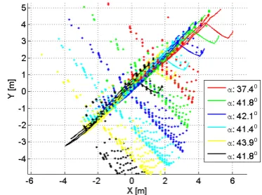
The same method can be applied to all of the consecutive scans resulting in a set of heading estimations. The results from a sample dataset, computed for every second scan, is shown in Figure 6. In this particular case, the mean and the median heading from these estimations are 41.5˚ and 41.7˚, respectively. The standard deviation of the heading is 1.9˚. Since 30% of the estimated orientations are not in the 1 range, removing these values, the mean orientation is 42.1˚ and the standard deviation is 0.7˚. These heading results are relative to the reference model, and thus have to be corrected by the absolute heading of the reference model to get the absolute heading.
Figure 6. Fitted consecutive scans and orientations
5. HEADING ESTIMATION USING ICP BETWEEN CONSECUTIVE SCANS
The relative displacements of the consecutive scans can be used to estimate the heading based on the equations of motion. As stated above, because of the small scanned area and the steadily moving aircraft, the heading and velocity are assumed to be constant between the entering and leaving points of the scanned area. Furthermore, since the aircraft is moving on the taxiway, we also consider no vertical movements, thus the goal is to extract the 2D motion parameters of the aircraft.
5.1 Algorithm
The following steps present the proposed algorithm for the derivation of the displacements and �, �.
Step 1. To achieve better performance, the point clouds were filtered before running one of the ICP algorithms. The goal of the filtering is to select the most “nearest” points found to the sensor in the Y direction. For this reason the X-Z plane is decimated into a grid of 0.1 x 0.1 m. Those points remain in the cloud which have the smallest coordinates inside one of the bins:
̂ = { | min�
, boundary limits of the bin in X, Y directions − +1= . , and
− +1= . .
Step 2. In order to estimate the ∆ �,�+ , ∆ �,�+ displacements, three implementations of ICP have been used (Rusinkiewicz, 2001; Geiger, 2012):
3D ICP: The applied well-known 3D ICP minimizes the point-to-plane distance metric between the corresponding (closest) points. This version of ICP estimates the 6 degree-of-freedom (DoF) rigid-body motion. These parameters can be extracted using singular value decomposition (SVD) approach.
3-DoF 3D ICP: Considering that the aircraft moves on the taxiway, the vertical motion can be neglected, thus it can be represented as a 2D problem. Here the heading and the offset parameters between the two scans have to be estimated, thus it is a 3-DoF rigid-body motion. The equations can be also solved using point-to-plane distance metric by SVD. Regarding the cost function, despite to the fact that the motion is restricted to a plane, the residuals are measured as the L2-norm of the 3D coordinates, and thus the objective function provides the total metric differences of the 3D points.
2-DoF 3D ICP: Under the assumptions that the heading and velocity are constant, only 2D displacements are estimated, and thus, the ICP has to provide only these parameters.
Step 3. ∆ �,�+, ∆ �,�+ and ∆�,�+ can be determined between all of the consecutive scans, which means − equations of Eq. 1:
cos � ∗ � ∗ ∆�,�+ − ∆ �,�+ =
sin � ∗ � ∗ ∆�,�+ − ∆ �,�+ = . (4)
Since errors are present, parameter estimation is required. Furthermore, robust estimation, such as RANSAC, is recommended to use in order to filter the outliers caused by failed ICP registrations.
5.2 Comparison of ICP solutions
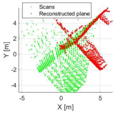
To eliminate the errors caused by non-overlapping clouds, those full 360-degree scans were selected as input to the algorithm which contain at least the 80% of the aircraft body. The ICP registration algorithm provides the reconstructed plane. Figure 7 shows the original point clouds and the reconstructed object from
the 2-DoF ICP with green and red dots, respectively. Note the aircraft fuselage, the wings, even the blades are easily identifiable, as well as, the contours are sharp, which indicates the good performance of the ICP. The other types of ICP generated a slightly similar point clouds.
Figure 7. Results of 2-DoF ICP
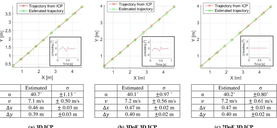
Figure 8 presents the quantitative results. The three columns show the results of the three ICP versions for a sample dataset. In the plots, the upper row, the red lines present the trajectories derived from the ICP, and the green lines show the trajectory calculated from the estimated �, �. The circles of the lines present the positions at different scans. The results indicate that the individual ICPs and the estimated parameters provide the same solutions. In other words, the model nearly perfectly fits to the estimated values, and thus, the circles have to be at the same location. The differences between the circles can be interpreted as the residuals of the ∆ , ∆ . These differences are small between the solutions. The lower right corner in Figure 8 presents the changes of the heading. These heading values are between
±1˚ and they seem to behave randomly; note no bias is
recognizable. It means these heading discrepancies can be interpreted as error “corrections” determined by the 3D and 3 -DoF ICP. As stated before in the 2--DoF case, the heading is not estimated, thus Figure 8c does not show any changes.
Also note the standard deviations of the heading predicted by error propagation equation is more than the realization in this dataset. It can be interpreted as this equation overestimates the heading error caused by ICP registration. In contrast, the accuracy of the velocity estimation follows the predicitions. Of course, the sample set is not sufficiently large to derive representative statistics regarding the validation of the error propagation model.
The statistical results are presented in the lower row in Figure 8, listing the heading and velocity parameters and the samples (translations). The statistics are calculated from the results of the consecutive ICPs. The standard deviations of the heading in the case of 3D, 3-DoF and 2-DoF ICP are ±1.13˚, ±0.97˚, and
±0.80˚, respectively. Note that the 2-DoF ICP solution has
marginally better statistical properties in heading estimation. In contrary, the ±0.50 m/s standard deviation of the velocities is slightly better in the 3D ICP case, but the estimated velocity is almost the same (7.2 m/s). The standard deviations of the translations are between 2-3 cm in all of the three cases.
Estimated σ
α 40.7˚ ±1.13 ˚
� 7.1 m/s ± 0.50 m/s
∆ 0.46 m ± 0.03 m
∆ 0.39 m ±0.03 m
Estimated σ
α 40.1˚ ±0.97 ˚
� 7.2 m/s ± 0.56 m/s
∆ 0.47 m ± 0.02 m
∆ 0.40 m ±0.02 m
Estimated σ
α 40.2˚ ±0.80˚
� 7.2 m/s ± 0.61 m/s
∆ 0.47 m ± 0.03 m
∆ 0.40 m ±0.02 m
(a) 3D ICP (b) 3DoF 3D ICP (c) 2DoF 3D ICP
Figure 8. Estimated parameters
Altough, no statistical differences can be detected on this dataset, 2-DoF 3D ICP is recommended to use due to its robustness if the motion assumptions are valid. In the solution presented in Figure 8, the overlapping between point cloud is provided. If the test sequence of the point clouds is extended with less overlapping clouds, the 3D ICP may fail; for instance, as shown in Figure 9. It is clearly seen that the 3D ICP (blue) detects a large pitch motion, and thus, the standard deviation of the heading drops down to ±10.57˚. In contrary, the 2-DoF 3D ICP depicted by red shows a better reconstructed plane shape, and the ±1.32˚ standard deviation of the heading estiamte is significatnly better.
Figure 9. Comparing the robustness of the 3D (blue) and the 2-DoF 3D ICP (red).
6. HEADING ESTIMATION WITH VOLUME MINIMIZATION
The idea behind this method is to make the reconstructed scene or object point cloud consistent. This consistency or the “disorder” can be measured by the entropy as it was introduced by Saez et al. Their approach was successfully applied in underwater and stereo vision scenarios (Saez, 2005, 2006). In these studies, the entropy is used for measuring the scene consistency after the preliminary pose and scene estimation. They minimize this entropy by ‘shaking’ the three pose coordinates and the three rotation parameters at every positions
quasi randomly. We use a similar approach, but in our case there are some constraints present, because all consecutive shots can be converted to the coordinate system of the first point cloud by assuming a certain � and � using the equation of motion (Eq. 1). In another words, the reconstructed plane can be determined if � and � are known, meaning that problem space is just 2-dimensional compared to Saez et al.,’s multidimensional space.
Generally the entropy can be estimated with decimating the space to equal-sided boxes (bins, cubes), see example in Figure 10a. Here, we use a different approach, namely volume minimization instead of entropy minimization, because we experienced slightly better results using this metric. Nevertheless, the entropy metric is also able to give acceptable results. In case of volume minimization, the “goodness” of the reconstruction is measured in the number of the boxes wherein at least one point is found. This metric aims at minimizing the space volume that is occupied by the point cloud.
See an example in Figure 10b, c. The left part shows the point cloud assuming � = 0˚ heading, and the “reconstructed” cloud results 865 boxes, as well as, the plane is hardly recognizable. The right part presents a more interpreable cloud and it resuls 275 boxes besides � = 45˚. This example also proved that this metric can be good for measuring the registration error.
The computational complexity of counting the occupied bins is linear to the number of the points, , where is the number of the points in the cloud. This complexity is significantly lower than that of the ICP’s objective function but the volume minimization is an ill-posed problem. In order to solve it, simulated annealing algorithm was used for finding the global minimum. The pseudo code of the algorithm is listed in Table 1. The simulated annealing is a stochastic optimization tool, which applies random numbers as heuristics. The cooling function, its parameterization, as well as, regulating the whole cooling process is important to get the right solution.
(a) Decimating the space into cubes (b) Point cloud at � = 45˚ resulting in 275 boxes and consistent cloud
(c) Point cloud at � = 0˚ resulting in 865 boxes and uninterpretable cloud
Figure 10. Examples for explaining the method of volume minimization
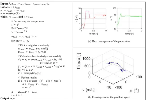
Table 1. The implemented simulated annealing algorithm for finding the mimimum volume respect to the headin and velocity, the convergence of the parameters are in the right side.
Input: , �� �, �� �, �, , �, , � , Initialize: ,
� ← �� �, � ← �� �
← entropy
while < and > �
// Decreasing the temperature ← �
� = �, * � = �, *
� ← �, � ← �
for = . .
// Pick a neighbor randomly
� ← � + �
� ← � + �
// Calculate the cloud (dynamic model)
′�← �+ cos � ∗ � ∗ ∆ ,� ∀
∈ [ ; ], �∈
′
�← �+ cos � ∗ � ∗ ∆ ,� ∀ ∈
[ ; ], �∈
′ ← entropy( ′�, ′�) // Update results
if ′< or exp − ′− >
� ← � , � ← �
← ′
� ← � , � ← �
← + Output: �, �
(a) The convergence of the parameters
(b) Convergence in the problem space
Variables: : point cloud, �, �∈ : th point from the point cloud, ∈ [ ; − ]: a random number, : maximum iteration number
(=150), : the entropy of the point cloud, �� �, �� �: initial guesses for the heading and velocity (=0,0), �, , �, : searching boundaries for heading and velocity (=90, 30), � : temperature that has to be achieved before return (=0.001), : number of neighbors to calculate at each iteration (=20), �, �: estimated heading and velocity (results), �: cooling schedule (geometric function), = . 5, note that ∈
; ], : temperature, �, �: radiuses for accessible neighbours ∆ ,�: time between the th and the first shot, � , � best parameters among the neighbours, � , � candidate parameters among the neighbors, ′�, ′�: coordinates of the th updated point
In our dataset, the geometric function is experienced to be the best cooling procedure. In order to avoid getting stuck at a local minima, we use exponential function in the update step. The right side of the figure shows the convergence of the parameters, and the convergence in the problem space which proves that the convergence is feasible. On the other hand, the method is a stochastic algorithm, thus different runs results slightly different solutions. For this reason, at each case, we run the algorithm, at least, 10 times and we used the statistics of these results to estimate the “goodness”or the “uncertainty”
of the method. Sometimes the algorithm gets stuck at a local minimum, say once in ten runs. These misidentifications are eliminated using sigma rule.
7. COMPARISON AND DISCUSSION The comparison of the three different methods, namely, heading estimation using reference model, Method 1, 2-DoF ICP, Method 2, and volume minimization, Method 3, are illustrated by an example in Figure 11.
Method 1 (using reference model) Method 2 (2-DoF ICP) Method 3 (volume minimization)
Figure 11. Comparison of the different solutions, top view
Because Method 1 does not provide any velocity estimation, the velocity from Method 3 is used for the cloud visualization. The estimated values can be seen under the plots. Figure 11 presents three datasets from three different object-sensor arrangements. The first dataset was captured at 10 m object distance with ~40˚ angle between the main scan plane and the motion direction. The second dataset shows a scenario at the same distance but with ~0˚ angle, and the last dataset was a challanging scenarios at 40 m object distance with ~0˚ angle and a realitively high velocity, ~ 7m/s, 12 knots, the maximum permitted at the test location.
On the first dataset, it is clearly seen that the different algorithms create comparable point clouds and similar estimation results. This proves that all approaches are able to provide the correct solution and the right feedback without reference solutions, such as GPS. The second and third datasets show that the sensor-object arrangement and distance can have relevant impact on the accuracy of the derived parameters and the reliability on the chosen method. The first dataset is presumably closely ideal for ICP algorithms due to the nearly 45˚ angle between the main scan plane and the motion direction of the aircraft. In this case the sensor can capture the whole 2D dimensional extensions (body and the wingspan) of the moving body, while at 0˚ angle it just sees the body, a cylindrical shape. ICP failures were exprencied in the latter cases, as it can be seen in the middle row of the table. The ICP method also fails if not enough points are acquired from the aircraft because of the long sensor-object distance, see last row. On the other hand, bigger aircraft with longer sensor-object distance provides the same amount of points as
smaller aircrafts in shorter range, thus in this case the ICP may be applicable.
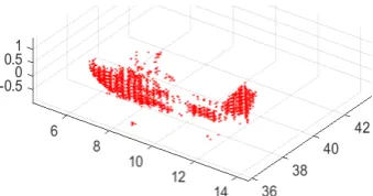
Surprisingly, the estimated heading parameter from Method 1 is consistent with the parameters derived from Method 3, even at larger distances, and not just on these three datasets, but on other investigated ones as well. The drawback of Method 1 is the use of a reference model, the aircraft types has to be known. In summary, Method 3 is the most reliable method. The final point cloud produced by Method 3 at the highest permitted speed and at the longest distance can be seen in Figure 12.
Figure 12. Point cloud from method 3 at ~7m/s velocity form 40 m object distance with ~0˚
In the future, we want to verify our methods with various types and sizes of aircraft operating at different distances. Additionally, more datasets are also essential to make the results statistically relevant. Installing multiple sensors are also able to improve the performance. On the other hand, the reference solutions are also required for comparative investigations. For this reason, we are planning to use GPS and IMU sensors on the airplane to compare the solutions.
8. CONCLUSION
3D active remote sensing, such as LiDAR technology, is able to provide excellent sensing capability to monitor operating aircrafts at airports. In this paper we used laser scanners with narrow vertical field of view to observe taxiing aircraft, and all results are based on using a Velodyne’s HDL-32E, for estimating the heading of the aircraft body. We investigated three different algorithms: the first uses reference model, the second is based on ICP algorithm, and the last one minimizes the volume of the reconstructed point cloud. We found that the volume minimization provides the most reliable and accurate solution, although reference solution is needed to verify the results.
Clearly, the LiDAR technology is able to sense aircraft body moving on the tarmac but during take-off and landing while in the air but close to the sensor. This solution opens new possibilities to centerline deviation monitoring and other safety studies. Furthermore, the fully reconstructed aircraft body can be used for determining other parameters, such as the aircraft type. These investigations are our middle/long term research plans.
ACKNOWLEDGEMENTS
Support from the FAA Pegasas Project 6 and the Center for Aviation Studies, OSU are greatly appreciated.
REFERENCES
Chou, C., Cheng, H., 2006. Aircraft Taxiing Pattern in Chiang Kai-Shek International Airport. In Airfield and Highway Pavement, pp. 1030-1040. doi: 10.1061/40838(191)87
Geiger, A., Lenz, P., Urtasun, R., 2012. "Are we ready for autonomous driving? The KITTI vision benchmark suite," In Computer Vision and Pattern Recognition (CVPR), 2012 IEEE Conference on , vol., no., pp. 3354,3361, 16-21 June 2012, doi: 10.1109/CVPR.2012.6248074
Huijing Z.; Shibasaki, R., 2005, "A novel system for tracking pedestrians using multiple single-row laser-range scanners," In: Systems, Man and Cybernetics, Part A: Systems and Humans, IEEE Transactions on Systems, Man and Cybernetics, vol.35, no.2, pp.283,291, March 2005 doi: 10.1109/TSMCA.2005.843396
Rosell J. R., Llorens J., Sanz R., Arnó J., et al., 2009, Obtaining the three-dimensional structure of tree orchards from remote 2D terrestrial LIDAR scanning, Agriculture and Forest Meteorology, Volume 149, Issue 9, 1 September 2009, Pages 1505–1515, DOI: 10.1016/j.agrformet.2009.04.008
Rusinkiewicz, Sz. , Levoy, M., 2001. “Efficient Variants of the ICP Algorithm”, in 3-D Digital Imaging and Modeling, pp.
145-152, URL:
http://www.cs.princeton.edu/~smr/papers/fasticp/fasticp_pap er.pdf
Scholz, F. 2003a. Statistical Extreme Value Analysis of ANC Taxiway Centerline Deviation for 747 Aircraft (prepared under cooperative research and development agreement between FAA and Boeing Company), URL: http://www.faa.gov/airports/resources/publications/reports/m edia/ANC_747.pdf
Scholz, F. 2003b. Statistical Extreme Value Analysis of JFK Taxiway Centerline Deviation for 747 Aircraft (prepared under cooperative research and development agreement
between FAA and Boeing Company) URL: http://www.faa.gov/airports/resources/publications/reports/m edia/JFK_101703.pdf
Scholz, F. 2005. Statistical Extreme Value Concerning Risk of Wingtip to Wingtip or Fixed Object Collision for Taxiing Large Aircraft (prepared under cooperative research and development agreement between FAA and Boeing Company),
Saez, J.M.; Escolano, F., 2005, Entropy Minimization SLAM Using Stereo Vision, Robotics and Automation, 2005. In ICRA 2005. Proceedings of the 2005 IEEE International Conference on Robotics and Automation, vol., no., pp.36-43, 18-22 April 2005, doi: 10.1109/ROBOT.2005.1570093
Saez, J.M.; Hogue, A.; Escolano, F.; Jenkin, M., 2006, Underwater 3D SLAM through entropy minimization In Robotics and Automation, 2006. ICRA 2006. Proceedings 2006 IEEE International Conference on Robotics and Automation, vol., no., pp. 3562-3567, 15-19 May 2006 doi: 10.1109/ROBOT.2006.1642246
Weiss, T.; Schiele, B.; Dietmayer, K., 2007, "Robust Driving Path Detection in Urban and Highway Scenarios Using a Laser Scanner and Online Occupancy Grids," Intelligent Vehicles Symposium, 2007 IEEE , vol., no., pp.184,189, 13-15 June 2007 doi: 10.1109/IVS.2007.4290112
Wilding et al., 2011. Risk Assessment Method to Support Modification of Airfield Separation Standards, ACRP Report 51 (prepared under airport cooperative research program,
sponsored by FAA) URL: