John C. Ham is at the University of Maryland, IFAU, IFS, IRP (Madison), and IZA. Daniela Iorio is at Universitat Autonoma de Barcelona and Barcelona GSE. Michelle Sovinsky is at the University of Zurich, the National University of Singapore and CEPR. The authors thank the editor and referees for comments which greatly improved the paper. They also thank Lynne Casper, James Heckman, Geert Ridder, Seth Sand-ers, Duncan Thomas and seminar participants at Alicante, Arizona, Chicago, Erlangen- Nuremberg, John Hopkins, IMT- Lucca, RAND, University of Southern California, Society of Economic Dynamics Meetings (Istanbul), the Econometrics Society Meetings (San Francisco), and the Econometrics Society European Meetings (Barcelona) for helpful comments. They are grateful to the National Science Foundation, the Claremont McKenna Lowe Institute for Political Economy, the USC College of Letters, Arts and Sciences, the Ministerio de Educacion y Ciencia (SEJ2006–00712), Ministerio de Ciencia y Tecnologia (SEJ2006– 00538), the Barcelona GSE, and the government of Catalonia for fi nancial support. Any opinions in this pa-per are those of the authors and do not necessarily refl ect the views of the NSF. The data used in this article can be obtained beginning January 2014 through December 2016 from michelle.sovinsky@gmail.com). [Submitted February 2011; accepted August 2012]
SSN 022 166X E ISSN 1548 8004 8 2013 2 by the Board of Regents of the University of Wisconsin System
T H E J O U R N A L O F H U M A N R E S O U R C E S • 48 • 3
Persistence and State Dependence of
Bulimia Among Young Women
John C. Ham
Daniela Iorio
Michelle Sovinsky
A B S T R A C T
Bulimia nervosa (BN) is a growing health concern and its consequences are especially serious given the compulsive nature of the disorder. However, little is known about the mechanisms underlying the persistent nature of BN. Using data from the NHLBI Growth and Health Study and instrumental variable techniques, we document that unobserved heterogeneity plays a role in the persistence of BN, but up to two- thirds of it is due to state dependence. Our fi ndings suggest that the timing of policy is crucial: Preventive educational programs should be coupled with more intense (rehabilitation) treatment at the early stages of the BN behaviors.
I. Introduction
an ED.1 In the past decade, 6–8.4 percent of female adolescents engaged in purging
behaviors (National Youth Risk Behavior 2005). Females who engage in BN typically start when they are in their teens or early twenties; however, the onset age appears to be dropping. Children are reporting bulimic behaviors at ever younger ages, and the behavior is increasingly seen in children as young as 10 (Cavanaugh and Ray 1999).
Bulimia is characterized by recurrent episodes of “binge- eating” followed by
com-pensatory purging.2 There are serious health consequences from these binge and purge
cycles, including electrolyte imbalances that can cause irregular heartbeats, heart
fail-ure, infl ammation and possible rupture of the esophagus from frequent vomiting, tooth
decay, gastric rupture, muscle weakness, anemia, and malnutrition (American Psy-chiatric Association 1993). The impact on adolescents and children is even more
pro-nounced due to irreversible effects on physical development and emotional growth.3
Our work is motivated by evidence that bulimics persist in their behaviors (Keel et al. 2003), which may have long- run effects on health outcomes and human capital accumulation. One possible reason that individuals may persist in BN is that starving,
bingeing, purging, and exercise increase β −endorphin levels, resulting in the same
chemical effect as that delivered by opiates. Along these lines, Bencherif et al. (2005) compare women with BN to healthy women of the same age and weight. They scan their brains using positron emission tomography after injection with a radioactive compound that binds to opioid receptors. The opioid receptor binding in bulimic women was lower than in healthy women in the area of the brain involved in pro-cessing taste, as well as the anticipation and reward of eating. This reaction has been found in other behaviors that exhibit substantial persistence, such as drug addiction and gambling. Finally, some studies in the biological literature suggest that there may be a genetic component to BN beyond the production of opioids (Bulik et al. 2003).
It is has not been examined whether the persistence of BN is due to individual heterogeneity (that is, some girls have persistent traits that make them more prone to
bulimic behavior, but they are not infl uenced by past experience) or true state
depen-dence (that is, past BN behavior is an important determinant of current BN behavior) (Heckman 1981). In this paper we exploit longitudinal data on individuals’ history of bulimic behavior and time- changing explanatory variables to separate state
depen-dence from individual heterogeneity in BN persistence. We fi nd that up to two- thirds
of BN persistence is due to true state dependence. Also, the impact of past behavior on current behavior is fourfold higher among African American girls, and girls from low- income households exhibit the highest persistence.
These fi ndings have important policy implications. Since true state dependence is
the most important cause of persistence in BN, it is reasonable to expect that the longer an individual experiences BN, the less responsive she will be to policy aimed at combatting the behavior. In this respect the timing of policy intervention is crucial: Preventive educational programs aimed at instructing girls about the deleterious health
1. Approximately 80 percent of BN patients are female (Gidwani 1997).
2. Binge- eating is the consumption of an unusually large amount of food (by social comparison) in a two- hour period accompanied by a loss of control over the eating process. Compensatory behavior includes self- induced vomiting, misuse of laxatives, diuretics, or other medications, fasting, or excessive exercise. BN is identifi ed with frequent weight fl uctuations.
effects of BN, as well as treatment interventions, will be most effective if provided
in the early stages.4 Moreover, because the role of state dependence is not the same
across racial and income groups, early intervention should pay special attention to African Americans and girls from low- income families. Second, making the case for BN exhibiting positive state dependence would help put those exhibiting BN on equal footing (from a treatment reimbursement perspective) with individuals abusing drugs or alcohol. In some states this is a current policy issue, since in several states treatment for alcoholism and drug addiction is covered but ED treatment is not covered or is
covered less generously.5 In fact, only 6 percent of people with bulimia receive mental
health care (Hoek and van Hoeken 2003), while a majority of states cover treatment
for alcoholism and drug addiction (Center for Mental Health Services 2008.)6 Finally,
there are potential long- run implications of ED behaviors on educational attainment given that eating disorders impact health outcomes. Recent work has shown that poor child health and nutrition reduces time in school and learning during that time. These
fi ndings suggest that policies aimed at improving health early in the process could also
serve to improve educational attainment.7
In order to investigate the persistence of BN, we estimate dynamic linear, Tobit, Ordered Probit, and Probit models that address the limited dependent nature of our measures of bulimic behavior. Our control variables are demographic variables and time- changing measures of perfectionism, distrust, and feelings of ineffectiveness, as
well as a poor body image in some specifi cations. The time- changing control variables
enable us to allow for endogenous past behavior. However, we also allow for the possibility that time- changing personality indices are correlated with an unobserved time constant individual effect since, for example, some medical studies have found that genetic factors may play a role in BN incidence (Lilenfeld et al. 1998; Bulik et al. 2003). Our approach of allowing personality traits to impact bulimic outcomes is in the same spirit as the literature on the impact of noncognitive skills and personality traits on economic outcomes (for example, Borghans et al. 2008). We also consider weak IV and overidentifying restrictions tests. Our restrictions pass these tests, and our estimates are robust to different estimation methods and identifying assumptions.
The outline of the paper is as follows. In Section II we present a literature overview. In Section III we describe the data and present basic statistics on BN persistence. In
Section IV we present our methodology and discuss identifi cation, while in Section V we present our results. We conclude in Section VI.
II. Literature Review and Background
In the social science literature, there are three papers on bingeing or purging behaviors. Hudson et al. (2007) and Reagan and Hersch (2005) focus on the prevalence of various types of ED behaviors among women and men. In a companion paper, Ham, Iorio, and Sovinsky (2011, hereafter HIS), we use data from the National Heart, Lung, and Blood Institute Growth and Health Study (hereafter NHLBI) to ex-amine which adolescent females are most at risk for BN in a multivariate framework. The NHLBI Growth and Health survey was an epidemiological study conducted by Striegel- Moore et al. (2000); they examined univariate correlations between BN and
race and between BN and parental education. HIS fi nd that African- Americans are
more likely than Whites to exhibit bulimic behaviors (consistent with Striegel- Moore et al. 2000) and that these effects remain after controlling for the education of the
parent, family income, and personality traits. However, HIS fi nd a more subtle
pat-tern from the interaction of income, class, and race: Low- and middle- income African American girls and low- income White girls are at substantially higher risk of bulimic behaviors than girls from other race- income groups.
The work in this paper differs from previous studies in the economics and epide-miology literatures along many important dimensions. First, we consider dynamic aspects of BN and distinguish between persistence due to individual heterogeneity and true state dependence, where we allow for racial and income differences in persis-tence. Furthermore, given that genetic factors may contribute to BN, persistence due to individual heterogeneity may be important. Our investigation of the relative roles of state dependence and individual heterogeneity is related to the existing empirical literature on this issue in other contexts (see, for example, Labeaga and Jones 2003; Gilleskie and Strumpf 2005; for a survey see Chaloupka and Warner 2000).
The large and growing literature on obesity is related to our work in the broad sense that it pertains to food consumption, but is otherwise unrelated given that women suffering from BN are characterized by average body weight (Department of Health and Human Services 2006). Our work is also related to the growing literature using
economic identifi cation strategies and appropriate econometric methods to investigate
public health issues, (see, for example, Adams et al. 2003; Engers and Stern 2002; Heckman et al. 2007; Hinton et al. 2010; Smith 2007). Finally, our work is different from previous research in the economics and epidemiology literature on habit
forma-tion in that we consider nonlinear and fi xed effects estimators appropriate for limited
dependent variables.
III. Data
organi-zation in the Washington, D.C. area.8 The survey was conducted annually for ten years
and contains substantial demographic and socioeconomic information such as age, race, parental education, and initial family income (in categories), as well as questions
on BN behavior. The latter were fi rst asked in 1990, when the girls were aged 11–12
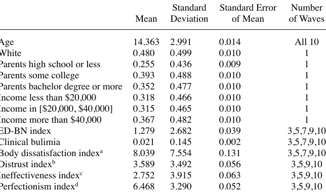
(Wave 3) and subsequently asked in Waves 5, 7, 9, and 10. We present descriptive statistics in Table 1. We include clustered standard errors of the mean to account for the fact that for all demographic variables (except age) we have one observation per person, while for the other variables we have multiple observations per person. The
survey is an exogenously stratifi ed sample, designed to be approximately equally
dis-tributed across race, income, and (highest educated) parental education level, as the
descriptive statistics in Table 1 confi rm.
The questions regarding bulimic behaviors were developed to be easy to
under-stand by young respondents and to be consistent with diagnostic criteria for BN.9
In particular, for each respondent the data contain an Eating Disorders Inventory index developed by a panel of medical experts, which was designed to assess the psychological traits relevant to bulimia (Garner, Olmstead, and Polivy 1983). Thus, a major advantage of these data is that all sample participants are evaluated regard-ing BN behaviors, and a BN eatregard-ing disorder index is developed for each participant independent of any diagnoses or treatment they have received. The survey reports an Eating Disorders Inventory Bulimia subscale for each respondent (hereafter the ED- BN index), which measures degrees of her behavior associated with BN. The ED- BN index is constructed based on the subjects’ responses (“always” = 1, “usu-ally” = 2, “often” = 3, “sometimes” = 4, “rarely” = 5, and “never” = 6) to seven items: 1) I eat when I am upset; 2) I stuff myself with food; 3) I have gone on eating binges where I felt that I could not stop; 4) I think about bingeing (overeating); 5) I eat moderately in front of others and stuff myself when they are gone; 6) I have the thought of trying to vomit in order to lose weight, and 7) I eat or drink in secrecy. A response of 4–6 on a given question contributes zero points to the ED- BN index; a response of 3 contributes one point; a response of 2 contributes two points; and a response of 1 contributes three points. The ED- BN index is the sum of the con-tributing points and ranges from 0 to 21 in our data. For instance, if a respondent answers “sometimes” to all questions, her ED- BN index will be zero. We have only the aggregate score, not the answers to individual questions. As Table 1 indicates, the mean ED- BN index is 1.2.
A higher ED- BN score is indicative of more BN related problems that are char-acterized by uncontrollable eating episodes followed by the desire to purge. Accord-ing to the team of medical experts that developed the index (Garner, Olmstead, and Polivy 1983), a score higher than 10 indicates that the girl is very likely to have a
8. The data do not report the location of the participant due to confi dentiality concerns. Schools were selected to participate in the study based on census tract data with approximately equal fractions of African American and White children where there was the least disparity in income and education between the two ethnic groups. The majority of the cohort was randomly drawn from families with nine- (or ten- ) year- old girls that participated in the Health Maintenance Organization (HMO). A small percentage was recruited from a Girl Scout troop located in the same geographical area as the HMO population.
clinical case of BN. The quantitative interpretation in terms of who is perceived to be suffering from clinical BN is motivated by results from surveys among women diagnosed with BN (by the Diagnostic and Statistical Manual of Mental Disorders
(DSM- IV) criteria): The average ED- BN index among this subsample was 10.8.10
For this reason, we will refer to a value of the ED- BN index of greater than 10 as clinical bulimia for the remainder of the paper. The ED- BN index is widely used in epidemiological and ED studies (Rush, First, and Blacker 2008). As shown in Table 1, approximately 2.2 percent of the girls (who are 14 years old on average) have a case
of clinical BN, which is close to the national average reported from other sources.11
However, in estimating some, but not all, of our models, we will exploit the fact that we know the numerical value of the index rather than simply whether it is greater
than 10; this tends to result in an effi ciency gain but does not change the basic nature
of our results.
The NHLBI Growth and Health survey also contains questions used to construct four other indices based on psychological criteria. These indices were developed by
10. See Garner, Olmstead, and Polivy (1983) for more details on the development and validation of the ED- BN index.
11. See, for instance, Hudson et al. (2007) and National Eating Disorders Association (2008). Table 1
Parents high school or less 0.255 0.436 0.009 1
Parents some college 0.393 0.488 0.010 1
Parents bachelor degree or more 0.352 0.477 0.010 1
Income less than $20,000 0.318 0.466 0.010 1
Income in [$20,000, $40,000] 0.315 0.465 0.010 1
Income more than $40,000 0.367 0.482 0.010 1
ED- BN index 1.279 2.682 0.039 3,5,7,9,10
Clinical bulimia 0.021 0.145 0.002 3,5,7,9,10
Body dissatisfaction indexa 8.039 7.554 0.131 3,5,7,9,10
Distrust indexb 3.589 3.492 0.056 3,5,9,10
Ineffectiveness indexc 2.752 3.915 0.063 3,5,9,10
Perfectionism indexd 6.468 3.290 0.052 3,5,9,10
Note: Income is in 1988$. See Appendix for more detailed description of the variables. a. This index ranges from 0 to 27 (maximal dissatisfaction).
a panel of medical experts (see Garner, Olmstead, and Polivy (1983) for a discussion of the association of these personality traits with EDs). The four additional indices measure a respondent’s potential for personality traits / disorders, and below we refer to
these indices collectively as the “personality indices.” The fi rst index is a measure of
each girl’s dissatisfaction with her body. This index is reported every year and is a sum of the respondents’ answers to nine items intended to assess satisfaction with size and
shape of specifi c parts of the body. Hereafter we refer to it as the body dissatisfaction
index. We also use three additional indices based on psychological criteria, measuring tendencies toward perfectionism (hereafter the perfectionism index), feelings of inef-fectiveness (hereafter the inefinef-fectiveness index), and interpersonal distrust (hereafter the distrust index). These indices are available in Waves 3, 5, 9, and 10, and thus overlap with the ED- BN index availability, with the exception that the ED- BN index is also available in Wave 7. For ease of exposition, we provide details on the questions used to form the personality indices in Appendix 1. In all cases we do not have the responses to the questions used to construct the score, just the aggregated index, where a higher score indicates a higher level of the personality trait.
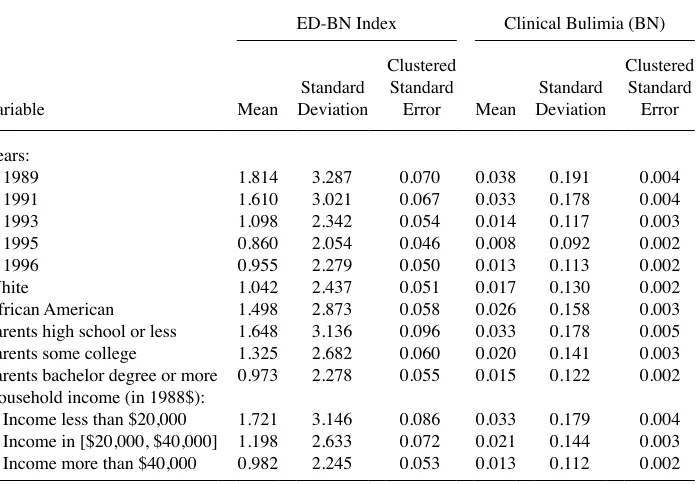
Table 2 shows the univariate relationship between the demographic variables, the ED- BN index (Columns 1–3), and BN incidence (Columns 4–6). Again, in each case we cluster the standard errors (by individual) for the means. The results indicate that as the girls age, both the ED- BN index and BN incidence fall. A notable point, which we examine in detail in our companion paper (HIS 2011), is that African American
girls have a statistically signifi cant higher ED- BN index and incidence of clinical BN
than White girls. Furthermore, both the ED- BN index and the incidence of clinical BN decrease as (the highest educated) parental education and family income increase,
and again these differences are statistically signifi cant at standard confi dence levels.
These results suggest that BN is more problematic among African American girls, girls from low- income families, and girls from families with low parental education. As we
discuss in HIS, these fi ndings are not due to an incorrect interpretation of what the
ED- BN index measures, that is, the possibility that it might capture obesity (binge
eat-ing) instead of BN behaviors. Neither do these fi ndings disappear once we condition
on the other demographic variables or personality indices. The bottom panel of Table 2 shows that both the ED- BN Index and BN incidence are correlated with the indices measuring personality traits.
IV. Empirical Models
some girls have persistent traits that make them more prone to bulimic behavior). We
fi rst consider a linear regression framework, since it allows an extended discussion
of identifi cation issues, which arise in any nonexperimental estimation of this type.
We then consider limited dependent variable models to estimate state dependence in bulimic behavior.
We consider four model specifi cations: (i) a linear regression structure that treats a
zero value of the ED- BN index as lying on the regression line; (ii) a Tobit structure for the ED- BN index; (iii) a linear probability model (LPM) for the incidence of clinical BN (that is, a value for the ED- BN index greater than 10) and (iv) a Probit model.
Table 2
Mean of ED- BN Index and Incidence of Clinical Bulimia by Characteristics
ED- BN Index Clinical Bulimia (BN)
Variable Mean
1989 1.814 3.287 0.070 0.038 0.191 0.004
1991 1.610 3.021 0.067 0.033 0.178 0.004
1993 1.098 2.342 0.054 0.014 0.117 0.003
1995 0.860 2.054 0.046 0.008 0.092 0.002
1996 0.955 2.279 0.050 0.013 0.113 0.002
White 1.042 2.437 0.051 0.017 0.130 0.002
African American 1.498 2.873 0.058 0.026 0.158 0.003
Parents high school or less 1.648 3.136 0.096 0.033 0.178 0.005 Parents some college 1.325 2.682 0.060 0.020 0.141 0.003 Parents bachelor degree or more 0.973 2.278 0.055 0.015 0.122 0.002 Household income (in 1988$):
Income less than $20,000 1.721 3.146 0.086 0.033 0.179 0.004 Income in [$20,000, $40,000] 1.198 2.633 0.072 0.021 0.144 0.003 Income more than $40,000 0.982 2.245 0.053 0.013 0.112 0.002
Correlations of ED- BN Index and Clinical Bulimia with Personality Characteristics
Personality Characteristic Index ED- BN Index Clinical Bulimia (BN)
Body dissatisfaction index 0.221 0.114
Distrust index 0.213 0.107
Ineffectiveness index 0.439 0.274
Perfectionism index 0.229 0.145
A. Linear Model
We begin with the regression model and consider our most basic specifi cation
(1) yit = α0+α1yit−1+δi+vit,
where yit−1 is the lag of the observed value of the ED- BN index, δi is an (unobserved)
individual- specifi c random effect, and vit is an uncorrelated (over time) error term. We
drop the year dummies for ease of exposition.12 The least squares estimate of α
1 will
refl ect both observed and unobserved heterogeneity as well as true state dependence.
To account for observed heterogeneity, we include current explanatory variables Xit to
obtain
(2) yit = γ0+ γ1yit−1+γ2Xit+δi+vit.
In our application Xit will consist of some or all of the current level of the
personal-ity characteristics (henceforth CPC) and the demographic variables (ethnicpersonal-ity, income, and the highest education of the parents) and in our basic model we assume that they
are uncorrelated with δi and with vit. We now consider issues related to identifi cation
to ensure that our estimate of γ1 refl ects only true state dependence.
1. Identifi cation
Identifi cation is an important and diffi cult issue in the estimation of dynamic models
since they often do not lend themselves to using experimental data to estimate the parameters of interest. Researchers generally face a number of options for achieving
identifi cation, none of which may be totally convincing on its own. Therefore, we
consider a number of identifi cation strategies to see whether our results are robust to
changing the identifi cation strategies. Our fi rst approach is to treat δi as a random
ef-fect uncorrelated with Xit, and to use the time- changing components of Xit−1 (that is,
the lagged personality characteristics, henceforth LPC) as excluded IV for the
endog-enous lagged dependent variable.13 Consider the case in which we use only one lag of
the personality characteristics as IV. Our approach will not produce consistent
esti-mates of γ1 if Xit−1 are weak instruments, that is, π2→ 0 as N → ∞ in the fi rst stage
equation,
(3) yit−1= π0+ π1Xit+ π2Xit−1+ eit−1.
Standard tests indicate that in our study Xit−1 are not weak instruments in the sense that
they affect yit−1 conditional on Xit (see Table 4).14 Thus, the validity of our identifi
ca-tion strategy, condica-tional on treating δi as a random effect uncorrelated with Xit, rests
on whether it is reasonable to assume that the LPC Xit−1 affect yit only through yit−1.
Suppose that this is not true in our data, and that the correct specifi cation is
12. If we add time dummies, the only real change is that age becomes very insignifi cant.
13. An alternative identifi cation strategy, which we did not investigate, is offered by Lewbel (2007). He shows that one does not need exclusion restrictions if one is willing to assume that the variance in the fi rst stage error term differs across individuals and depends on observable characteristics while the covariance between the fi rst stage and second stage error terms is constant.
(4) yit = γ0+ γ1yit−1+γ2Xit+ γ3Xit−1+δi+ νit.
However, if Equation 4 holds, we expect the overidentifying test for Equation 2 to fail. To see this consider a “reduced form” version of Equation 2 for current BN behavior
(5) yit = ρ0+ρ1Xit +ρ2Xit−1+ eit.
The overidentifying restriction test considers the null hypothesis ρ2 = γ1π2, which we
would not expect to hold if Equation 4 is the correct model. We do not fail these tests,
and thus we conclude that the data suggest that Xit−1 affects yit only through yit−1.15
Finally, one may be concerned that δi is correlated with Xit. An extreme version of
this issue has been raised in the medical literature, where, as noted above, it is
hypoth-esized that Xit, Xit−1 and yit are a function of a single unobserved factor, plus a random
noise. To consider this, let
(6) yit = αi+vit,
where αi is iid across i and has mean 0 and variance σα2,v
it is iid across i and t with
mean 0 and variance σv2, and E α
i,vi't
(
)
= 0 for all i,i′ and t. Further, assume thatper-sonality characteristic k,Xkit, is determined by
(7) Xkit = φkαi+ ekit, k =1, ...,K,
where E(vitekiτ) = 0 and E(ekiτek''i'τ) = 0 for all
i,i′,t,τ and k ≠ k′. Given the true value
of each βk is zero, we can consider the regression
(8) yit =βXit+αi+vit,
where αi is treated as a random effect uncorrelated with Xit. However, the least squares
coeffi cients are biased, that is, E(β)≠ 0, because
(9) E X
[
kit(
αi+ vit)
]
= E[
(
φkαi+ekit)
(
αi+vit)
]
= φkσα2, k = 1, ...,K.If we fi rst difference the equations for yit and Xit we obtain
(10) ∆yit = β∆Xit +∆vit,
where ∆ represents the fi rst- difference operator. Now the least squares coeffi cients are
unbiased, that is, E(β) = 0, because
(11) E
[
∆Xkit∆vit]
= E[
∆ekit∆vit]
= 0 for all k =1, ...,K..To investigate the single factor hypothesis, we estimate Equation 10 and test the null
hypothesis β = 0 for each specifi cation considered below. We decisively reject the null
hypothesis β = 0 in all cases and thus conclude that the single factor model is not
ap-propriate in our application.16
We next consider a specifi cation of our general model given by Equation 2 where it
is appropriate to treat δi as a fi xed effect (FE). As is well known, care must be
exer-15. This, of course, assumes that the overidentifying tests are not passed simply because of a lack of power. 16. When we do not include body dissatisfaction in the personality characteristics, the Wald statistics for the null hypothesis β = 0 when we use (do not use) the interpolated data are 190.652 (128.498), which are both much bigger than any reasonable critical value for χ2(3). When we include body dissatisfaction in the
cised when estimating FE dynamic models. To obtain consistent estimates, we follow
Arellano and Bond (1991; hereafter AB) and eliminate the FE by fi rst differencing
Equation 2 to obtain
(12) ∆yit = β0+β1∆yit−1+β2∆Xit + ∆vit.
We consider two cases. First, we assume that vis is independent of Xit for any t
condi-tional on δi, i.e., Xit is strictly exogenous (Wooldridge, 2002, p. 253). Under this
as-sumption we can treat ∆Xit as exogenous in Equation 12 and Xit−1 as excluded IV, that
is, ∆Xit acts as its own instrument. However, often these will be weak IVs, and this
indeed is a problem in our application. AB consider this problem and suggest that
re-searchers also use yit−2 as an IV. Note that the lag of the dependent variable will be a
valid IV as long as vit is independent over time. AB stress the importance of specifi
ca-tion tests in using this assumpca-tion for identifi cation. Specifi cally, one can test the null
hypothesis that vit is independent over time, as well as the null hypothesis that the
overidentifying restrictions hold. We fi nd we do not reject either of these null
hypotheses.17
AB note that the use of yit−2 as an IV allows one to make weaker assumptions on the
Xit. For example, there may be feedback effects from vit to future values of Xit and in
this case strict exogeneity would no longer hold. To address this potential issue, we
assume only sequential exogeneity, that is, that vis is independent of Xit only for s≥ t
conditional on δi (Wooldridge 2002, p. 299). Under the sequential exogeneity
assump-tion, we estimate the parameters of Equation 12 by 2SLS while also treating ∆Xit as
endogenous; we use yit−2 and Xit−1 as our excluded IV. We fi nd that for this specifi
ca-tion we also cannot reject the null hypothesis that vit is independent over time, nor can
we reject the overidentifying assumptions.18 Below we fi nd that these different
ap-proaches produce similar estimates of true state dependence, presumably increasing
the confi dence readers can place in our estimates.
B. Tobit Model
For the Tobit model, we start by considering the simplest latent variable equation
(13) yit* = λ
0+λ1yit−1+μi+eit,
where μi are (unobserved) individual- specifi c random effects and eit is an uncorrelated
(over time) error term, both of which are normally distributed. The estimate of λ1 will
capture observed and unobserved heterogeneity and true state dependence. To account
for observed heterogeneity, we add explanatory variables Xit to obtain
(14) yit* = θ
0+θ1yit−1+θ2Xit +μi+eit,
17. Again we need to add the caveat that we may not reject these null hypotheses simply because of a lack of power.
where the estimate of θ1 will refl ect unobserved heterogeneity and true state depen-dence. To capture only the latter, we consider the Wooldridge (2005) dynamic corre-lated random effects Tobit model based on Chamberlain (1984), and assume that
(15) μi = ϕ3Xi+ϕ4yi0+ci,
where Xi denotes the mean value of the explanatory variables, yi0 the initial condition,
and ci an individual specifi c error term. We now have
yit* = ϕ
0+ϕ1yit−1+ϕ2Xit+ϕ3Xi+ϕ4yi0+ ci+eit.
We estimate the model by following Wooldridge (2005) in assuming strict exogeneity
for the Xit (with respect to eit) and then using MLE; in this case, the estimate of ϕ1
re-fl ects only true state dependence. Restricting the initial condition to depend on the
initial observation of the ED- BN index is less of a problem in our sample because we have data on the respondents when they are young, and hence it seems reasonable to
assume that yi0 captures initial conditions.
As a robustness check we also estimate a dynamic Probit model (using the Wooldridge procedure) and a dynamic LPM for the incidence of the ED- BN index being greater than 10. For the LPM, we proceed in a manner analogous to the linear regression model, and for the Probit model, we proceed in a manner analogous to the Tobit. See Appendix 2 for details.
V. Empirical Results
A. Results for the Linear Model
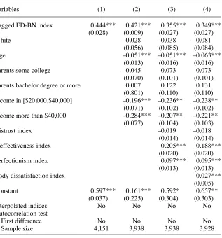
Table 3 contains our parameter estimates for the linear model. In Column 1 we con-sider a model where the only explanatory variable is the (assumed to be exogenous)
lagged dependent variable; its coeffi cient is estimated at 0.44 and, not surprisingly, it
is very statistically signifi cant. Regarding the effect of past ED- BN experience on
current behavior, the coeffi cient can be interpreted as an elasticity since we would
expect the mean of a variable and its lag to be equal. We obtain a relatively large
esti-mate of the elasticity of 0.44. To look at the magnitude of the coeffi cient in another
way, an individual with a lagged ED- BN index of 5 would have a current ED- BN
in-dex over two points higher than someone with a lagged inin-dex of 0; this difference is
almost 150 percent of the mean value of the ED- BN index. After we add the demo-graphic variables in Column 2 and the personality indices in Column 3, the lag
coef-fi cient drops to 0.421 and 0.35, respectively, and is insensitive to including body
dis-satisfaction in Column 4. These results demonstrate substantial persistence in BN behavior that can be due to both unobserved heterogeneity and true state dependence.
To focus on the latter, we fi rst assume the individual effect in Equation 2 is
uncor-related with Xit. As noted above, in this case researchers can use Xit−1 as IV as long as
they are not weak IV. Fortunately, in our case Xit−1 are not weak instruments, and thus
we do not need to add yit−2 as an IV, which would require restrictions on the
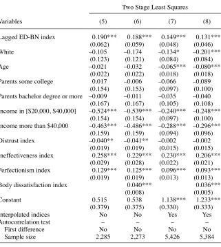
covari-ance of vit over time for the same individual. Thus in Columns 5 to 8, we estimate
Equation 2 while treating the lagged dependent variable as endogenous and use Xit−1
the fi rst and second stage equations, while in Column 6 we include body
dissatisfac-tion. Columns 5 and 6 both report a lagged coeffi cient of approximately 0.2,
suggest-ing that over half the variation in persistence attributed to unobserved heterogeneity
and state dependence is actually due to the latter. The coeffi cient estimate of 0.2
sug-gests an elasticity of 0.2 for the effect of lagged BN on current behavior. To put this another way, the expected ED- BN index for someone who has a lagged value of the ED- BN index equal to 5 compared to someone who has a lagged value of 0 would be
higher by 1, approximately 80 percent of the mean value of 1.2.19
19. Some girls in our sample may receive treatment once they begin bulimic behavior, although we cannot identify who they are. If this treatment is even partially effective, it will reduce the degree of true state depen-Table 3
Linear Regression Estimates of the Persistence of ED- BN Index
Variables (1) (2) (3) (4)
Lagged ED- BN index 0.444*** 0.421*** 0.355*** 0.349***
(0.028) (0.009) (0.027) (0.027)
White –0.028 –0.038 –0.081
(0.056) (0.085) (0.084)
Age –0.051*** –0.051*** –0.063***
(0.013) (0.016) (0.016)
Parents some college –0.045 0.073 0.073
(0.070) (0.101) (0.101)
Parents bachelor degree or more 0.007 0.122 0.131
(0.801) (0.110) (0.110)
Income in [$20,000,$40,000] –0.196*** –0.236** –0.238**
(0.071) (0.102) (0.102)
Income more than $40,000 –0.284*** –0.207** –0.221**
(0.077) (0.104) (0.103)
Distrust index –0.019 –0.018
(0.014) (0.014)
Ineffectiveness index 0.205*** 0.188***
(0.020) (0.020)
Perfectionism index 0.097*** 0.095***
(0.013) (0.013)
Body dissatisfaction index 0.027***
(0.005)
Constant 0.597*** 0.161*** 0.592* 0.657**
(0.037) (0.225) (0.304) (0.303)
Interpolated indices No No No No
Autocorrelation test
First difference No No No No
Sample size 4,151 3,938 3,938 3,928
Our sample size is limited by the fact that the personality indices are not available
in Wave 7, and this limitation is especially important in our AB analysis.20 However,
we can increase our sample size if we assume that the personality index values vary smoothly from Wave 5 to 9, and use interpolated values Wave 7, which doubles our
dence, so our estimates are lower bounds on the degree of true state dependence in untreated BN.
20. Specifi cally, in the AB analysis we lose the independent variables ∆Xit when the dependent variable is yi9 – yi7 and when the dependent variable is yi10 – yi9.
Table 3 (continued)
Two Stage Least Squares
Variables (5) (6) (7) (8)
Lagged ED- BN index 0.190*** 0.188*** 0.149*** 0.131***
(0.062) (0.059) (0.048) (0.046)
White –0.105 –0.174 –0.134* –0.201***
(0.123) (0.121) (0.084) (0.084)
Age –0.021 –0.032 –0.065*** –0.080***
(0.022) (0.022) (0.018) (0.018)
Parents some college 0.017 –0.006 –0.066 –0.089
(0.154) (0.153) (0.097) (0.100)
Parents bachelor degree or more –0.009 –0.011 –0.035 –0.040
(0.167) (0.167) (0.105) (0.108)
Income in [$20,000, $40,000] –0.524*** –0.539*** –0.240*** –0.248***
(0.154) (0.154) (0.097) (0.100)
Income more than $40,000 –0.463*** –0.486*** –0.288*** –0.296***
(0.159) (0.159) (0.094) (0.096)
Distrust index –0.040** –0.041** –0.002 –0.002
(0.019) (0.019) (0.015) (0.015)
Ineffectiveness index 0.258*** 0.229*** 0.230*** 0.206***
(0.029) (0.028) (0.022) (0.021)
Perfectionism index 0.129*** 0.125*** 0.096*** 0.093***
(0.019) (0.019) (0.013) (0.013)
Body dissatisfaction index 0.040*** 0.036***
(0.008) (0.005)
Constant 0.515 0.538 1.138*** 1.233***
(0.379) (0.375) (0.330) (0.333)
Interpolated indices No No Yes Yes
Autocorrelation test – – – –
First difference No No No No
Sample size 2,285 2,273 5,426 5,384
sample size.21 The 2SLS estimates of our basic model using the imputed data (with
and without body dissatisfaction) are in Columns 7 and 8. Comparing the results in Columns 7 and 8 to those in Columns 5 and 6, respectively, indicates that using the
imputed data diminishes the role of true state dependence by about one- fi fth, but that
the coeffi cient on the lagged value is still highly signifi cant.22 The interpolated indices
also allow us to use Xt−1 and Xt−2 as instruments. When we do this, we obtain
esti-21. When we use the interpolated indices we obtain a lagged ED- BN index coeffi cient of 0.327(0.022) and 0.323(0.022), for Columns 3 and 4, respectively. These estimates indicate that the results are very robust to the use of interpolated indices.
22. We also investigate whether the results are robust when we control for depression. We have self- reported information on depression in two waves. Using this subsample, we estimate the model with and without Table 3 (continued)
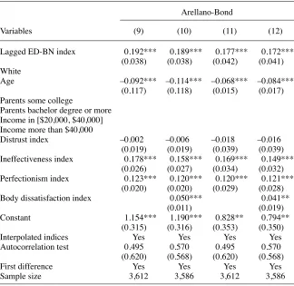
Arellano- Bond
Variables (9) (10) (11) (12)
Lagged ED- BN index 0.192*** 0.189*** 0.177*** 0.172***
(0.038) (0.038) (0.042) (0.041)
White
Age –0.092*** –0.114*** –0.068*** –0.084***
(0.117) (0.118) (0.015) (0.017)
Parents some college
Parents bachelor degree or more Income in [$20,000, $40,000] Income more than $40,000
Distrust index –0.002 –0.006 –0.018 –0.016
(0.019) (0.019) (0.039) (0.039)
Ineffectiveness index 0.178*** 0.158*** 0.169*** 0.149***
(0.026) (0.027) (0.034) (0.032)
Perfectionism index 0.123*** 0.120*** 0.120*** 0.121***
(0.020) (0.020) (0.029) (0.028)
Body dissatisfaction index 0.050*** 0.041**
(0.011) (0.019)
Constant 1.154*** 1.190*** 0.828** 0.794**
(0.315) (0.316) (0.353) (0.350)
Interpolated indices Yes Yes Yes Yes
Autocorrelation test 0.495 0.570 0.495 0.570
(0.620) (0.568) (0.620) (0.568)
First difference Yes Yes Yes Yes
Sample size 3,612 3,586 3,612 3,586
mated coeffi cients (standard errors) of 0.252 (0.071) and 0.177 (0.066), respectively for Columns 7 and 8 of Table 3.
As is standard practice, we consider two diagnostics for our 2SLS estimates in Col-umns 5 to (8). Table 4 presents the reduced form estimates to investigate the issue of
weak instruments. There will be heteroskedasticity in the fi rst- stage regression
equa-tion for a censored dependent variable; therefore, the widely used rule of thumb for the
fi rst- stage F- statistic of excluded instruments (Staiger and Stock 1997, Stock and Yogo
2005) will be inappropriate. Instead, we use the conjecture by Hansen, Hausman, and
Newey (2008) that in the presence of heteroskedasticity in the fi rst- stage equation, the
Wald statistic for the null hypothesis that the excluded instruments are zero in the fi rst
stage, minus the number of instruments, should be greater than 32. Note fi rst that we
pass the weak IV test in all specifi cations, and that the perfectionism, ineffectiveness,
and body dissatisfaction (when used) indices are always individually signifi cant,
sug-gesting that they are not simply driven by a single (genetic) factor.23
Further, when we consider the instruments on an individual basis, we pass the weak
IV test for the perfectionism, ineffectiveness, and body dissatisfaction indices.24
Our second diagnostic pertains to the overidentifi cation restrictions. We present a
Wald statistic to test the overidentifi cation restrictions that the instruments are valid,
which is suitable with heteroskedasticity and clustering; here the critical value is χ2(l),
where l is the degree of overidentifi cation. Intuitively, the test can be thought of as
assuming that one of the instruments is valid, and then examining whether the other
instruments have zero coeffi cients in the structural equation. Also, we specifi cally test
the validity of body dissatisfaction as an instrument, conditional on the other personal-ity indices being valid, by entering its lagged value as an explanatory variable in
Column 6 and testing whether its coeffi cient is signifi cantly different from zero. As the
p- values show, we can not reject the null hypothesis that the overidentifying restriction
with respect to restricting lagged body dissatisfaction is valid. Thus, overall the diag-nostics show that our instruments are not weak and the overidentifying restrictions, including that for body dissatisfaction in Column 6, are not rejected.
The 2SLS estimates in Columns 5 to 8 of Table 3 are consistent if we assume that
vis and δi are independent of Xit for all s,t. As noted above, to relax this assumption we also present the results using the AB approach of differencing before using 2SLS to
allow for the personality indices to be correlated with δi. We fi rst assume that the
personality traits are strictly exogenous with respect to vit in Equation 2) (That is, that
the personality traits are uncorrelated with vis at all s,t.) In this case we treat ∆Xit as
exogenous and use yit−2 and ∆Xit as excluded IV under the assumption that the vitare
independent over time. The results are in Columns 9 and 10 of Table 3 when we ex-clude and inex-clude body dissatisfaction, respectively. The results in Column 9 show a
highly signifi cant lag coeffi cient of around 0.19 and the coeffi cient estimates remain
the same when we include body dissatisfaction as an explanatory variable in Column
depression. The coeffi cient of the lagged ED- BN index is virtually the same and statistically signifi cant in both cases.
The Journal of Human Resources
Table 4
First Stage Estimates for Table 3
Estimates Corresponding to Columns 5–8 of Table 3
(1) (2) (3) (4)
Instruments for lagged ED- BN index
Lagged perfectionism index 0.154*** 0.154*** 0.165*** 0.165***
(0.019) (0.019) (0.014) (0.014)
Lagged ineffectiveness index 0.262*** 0.228*** 0.250*** 0.220***
(0.018) (0.019) (0.013) (0.014)
Lagged distrust index 0.017 0.013 –0.002 –0.006
(0.020) (0.020) (0.015) (0.015)
Lagged dissatisfaction index 0.060*** 0.053***
(0.011) (0.007)
Other regressors
White –0.221* –0.194 –0.249*** –0.282***
(0.130) (0.130) (0.080) (0.080)
Age –0.060** –0.083*** –0.078*** –0.106***
(0.027) (0.027) (0.018) (0.019)
Parents some college –0.181 –0.212 –0.171* –0.198**
Sovinsky
, Ham, and Iorio
753
Income in [$20,000, $40,000] 0.026 –0.021 –0.227** –0.230**
(0.159) (0.158) (0.096) (0.095)
Income more than $40,000 0.013 –0.041 –0.248** –0.263***
(0.171) (0.170) (0.103) (0.102)
Distrust index 0.040** 0.051*** 0.023 0.031**
(0.019) (0.019) (0.015) (0.015)
Ineffectiveness index 0.053*** 0.051*** 0.032** 0.028**
(0.017) (0.018) (0.013) (0.014)
Perfectionism index 0.005 0.004 –0.019 –0.020
(0.018) (0.018) (0.014) (0.014)
Body dissatisfaction index –0.020* –0.012*
(0.010) (0.006)
Constant 0.619 0.829* 1.350*** 1.640***
(0.453) (0.452) (0.327) (0.328)
Weak IV test statistic a 143 165 222 265
Overidentifi cation test b 1.796 2.005 2.736 3.096
(0.407) (0.571) (0.213) (0.407)
Interpolated values No No Yes Yes
Sample size 2,285 2,273 5,426 5,384
Note: Standard errors robust to heteroskedasticity and intra- group correlation reported in parenthesis. * indicates signifi cant at 10 percent level; ** signifi cant at 5 percent level; *** signifi cant at 1 percent level.
a. Hansen, Hausman, and Newey (2008) suggest that, in the presence of heteroskedasticity in the fi rst stage equation, the test statistic should be greater than 32.
10.25 The test of the null hypothesis of no serial correlation is essentially a test of the
overidentifying restriction on the lagged dependent variable (after allowing for heteroske-dasticity). From the bottom of Columns 9 and 10 we see that we cannot reject the null hypothesis, indicating that values of the ED- BN index lagged two periods (or more) are
valid instruments in the equations in fi rst differences, and our AB estimates are consistent.
Next we relax the strict exogeneity restriction by assuming that the personality traits
are sequentially exogenous in the sense that we only assume E(Xitvis)= 0 for t ≤ s to
allow for feedback from current vis to future Xit. Note that relaxing strict exogeneity
implies we must treat ∆Xit as endogenous in Equation 12, and we use yit−2 and Xit−1 as
excluded IV in the fi rst- differenced equation. The AB results for this case are in
Col-umns 11 and 12 when we exclude and include body dissatisfaction, respectively. Again, the test for serial correlation suggests that lagged two periods (or more) value
of the ED- BN index is a valid instrument.26 The coeffi cient of the lagged dependent
variable is estimated at 0.18 in Columns 11 and 12.
When carrying out IV estimation, it is not possible to test whether a model is
identi-fi ed (although it is possible to test over- identifying restrictions). However, the results
from diagnostic and robustness checks help us to add support to the notion that our
model specifi cation and identifying assumptions are appropriate. The estimates
ob-tained in Columns 5–12 are robust to a number of different identifi cation strategies in
terms of our assumptions on the independence of the personality traits Xit with respect
to δi and vit in Equation 2, and with respect to whether we include body dissatisfaction
in the model. Further, in terms of diagnostics, each of the different specifi cations
passes weak IV and overidentifi cation tests. Note in particular that our results are
ro-bust to allowing for the possibility (i) that personality indices are driven by a genetic
component in δi, that is, all personality traits are driven by one factor, and (ii) that there
may be feedback from current shocks to future values of personality indices.
In summary, we fi nd that there is substantial persistence in BN, and that about half
of this persistence is due to true state dependence. Further, the magnitude of the effect suggests that state dependence is quite important. Finally, these results are robust to
changes in the explanatory variables and identifi cation strategy.
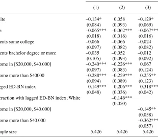
So far we have focused on models where state dependence is constant across race and income class. Table 5 presents 2SLS estimates describing the racial and income differences in the persistence of BN when we address the endogeneity of past behav-ior. We use interpolated values for Wave 7 (since we are estimating a richer model) and exclude body dissatisfaction as an explanatory variable. To facilitate the com-parison with these results, Column 1 repeats the results of Table 3 Column 7, where the lag is not interacted with race or income. In the remaining columns, we use the socioeconomic indicator of focus interacted with the lag of the perfectionism and ineffectiveness indices as IV. For example, in Column 2 we allow the persistence to differ by race, where the IV are race interacted with the lagged personality indices. Column 2 indicates that much of the persistence in the overall sample is driven by the behavior of African American girls. Indeed, the estimate for persistence among
Whites is very small and signifi cant (0.05), while it is substantial and signifi cant for
25. Weak instruments are not an issue because of the lagged dependent variable.
African- Americans (0.21). In Column 3, where we consider income differences in persistence, we observe that the strongest persistence is in low- income families, as
the estimated coeffi cient on the lagged behavior is signifi cant and very large at 0.32
(given we are instrumenting and imputing personality indices). It falls to 0.17 for middle- income families and is essentially zero for girls from high- income families.
These results show interesting race and income effects of BN persistence.27
B. Results for the Tobit and Other Nonlinear Models
The Tobit partial effect estimates are given in Table 6. Column 1 presents estimates where the only explanatory variable is the lagged dependent variable, and the estimated
27. The data are not rich enough for a model with race- income interactions in the levels and in the persis-tence.
Table 5
Racial and Income Class Differences in the Persistence of BN
Two- Stage Least Squares Estimates
(1) (2) (3)
White –0.134* 0.058 –0.129*
(0.084) (0.093) (0.069)
Age –0.065*** –0.062*** –0.067***
(0.018) (0.016) (0.016)
Parents some college –0.066 –0.066 –0.024
(0.097) (0.082) (0.082)
Parents bachelor degree or more –0.035 –0.052 –0.012
(0.105) (0.093) (0.092)
Income in [$20,000, $40,000] –0.240*** –0.226*** 0.067
(0.097) (0.083) (0.124)
Income more than $40000 –0.288*** –0.259*** 0.255**
(0.094) (0.089) (0.123)
Lagged ED- BN index 0.149*** 0.206*** 0.318***
(0.048) (0.036) (0.042)
Interaction with lagged ED- BN index, White –0.146***
(0.050)
Income in [$20,000, $40,000] –0.145**
(0.058)
Income more than $40,000 –0.362***
(0.057)
Sample size 5,426 5,426 5,426
The Journal of Human Resources
Tobit Partial Effects Estimates for the Persistence of the ED- BN Index
Variables (1) (2) (3) (4) (5)
Lagged ED- BN index 0.270*** 0.200*** 0.184*** 0.190*** 0.180***
(0.013) (0.012) (0.009) (0.013) (0.013)
White –0.077 –0.104**
(0.070) (0.060)
Age –0.041*** –0.036***
(0.013) (0.067)
Parents some college 0.096 0.035
(0.083) (0.067)
Parents bachelor degree or more 0.127 0.065
(0.095) (0.079)
Income in [$20,000,$40,000] –0.224*** –0.160***
(0.076) (0.065)
Income more than $40,000 –0.169** –0.160***
(0.086) (0.065)
Distrust index –0.007 –0.001 –0.015 –0.015
(0.010) (0.009) (0.012) (0.012)
Ineffectiveness index 0.123*** 0.118*** 0.114*** 0.099***
(0.010) (0.009) (0.011) (0.011)
Perfectionism Index 0.066*** 0.060*** 0.092*** 0.044***
(0.009) (0.008) (0.013) (0.018)
Body Dissatisfaction Index 0.019*** 0.033***
(0.003) (0.007)
Interpolated indices No No No No No
Chamberlain / Wooldridge No No No Yes Yes
Fixed effects
Sample size 4151 3938 3928 3938 3928
partial effect is 0.27. In Columns 2 and 3 we control for observable heterogeneity by including demographic variables and personality indices without and with body dissat-isfaction respectively. The partial effect of the lagged dependent variable falls to 0.20
in both Columns 2 and 3.28 In order to control for unobserved heterogeneity in
Col-umns 4 and 5, we include correlated random effects using the Wooldridge (2005) ap-proach, where we exclude and include body dissatisfaction, respectively. The estimates of 0.19 and 0.18 of the partial effect of the lagged dependent variable in these two col-umns capture true state dependence, and represent about two- thirds of BN persistence,
estimated at 0.27 in Column 1, which refl ects observed heterogeneity, unobserved
het-erogeneity, and true state dependence. Further, the persistence estimates in Columns 4 and 5 are approximately equal to those in Columns 2 and 3 respectively, suggesting that state dependence plays a much larger role than unobserved heterogeneity.
The estimated partial effects from the Probit and LPM models are of the same sign as the linear and Tobit estimates (see Tables A2 and A3 in Appendix 2), but fewer
estimated coeffi cients are statistically signifi cant. This is expected since the Probit
and LPM use much less information per person. Indeed, our estimates illustrate the importance of not focusing only on whether an individual has BN for understanding the determinants of the disorder.
VI. Conclusions
This is the fi rst study that quantifi es the role of true state dependence
and individual heterogeneity in bulimia nervosa among adolescent girls. We use a panel data set, the NHLBI Growth and Health Survey, which is uniquely suited for studying these issues. A major advantage of these data is that all sample participants were evaluated regarding bulimic behaviors for ten years, starting when they were young (aged 11–12 years), independent of any diagnoses or treatment they had re-ceived. For each respondent, the data contain i) an Eating Disorders Inventory index, developed by medical experts; ii) information on SES, and iii) information on time- changing personality traits.
Our use of these data produces a number of important results. First, and perhaps
most importantly, we fi nd that much of the persistence in bulimic behavior is due
to true state dependence after controlling for individual heterogeneity, and that this result continues to hold when we allow for the possibility that the personality traits are correlated with an individual random effect (possibly driven by a genetic factor), and the possibility that there is feedback from the current shock in BN to future values of
the personality indices. Indeed we fi nd that up to two- thirds of the persistence in BN
is due to the true state dependence, and that the past four years of behavior positively
and signifi cantly impact bulimic behavior in the current period.
Further, we show that African- Americans are more likely to persist in bulimic be-havior relative to Whites. Indeed, the estimates suggest that the impact of past behav-ior on current behavbehav-ior is fourfold higher among African- Americans. In addition, the strongest persistence (among income groups) is present in low- income families.
Our results have several important policy implications. First, since state dependence plays an important role in BN persistence, it is reasonable to expect that the longer an individual experiences BN, the less responsive she will be to policy aimed at combat-ing it. In this respect it is important to instruct a wide range of young women on the deleterious effects of BN and the importance of getting help, especially at the initial stages of bulimic behaviors. In addition, to the extent that poor health is linked with lower educational attainment, policy aimed at combating the onset of bulimic behav-iors among young girls could also serve to improve educational attainment.
Finally, a number of aspects of BN behavior are consistent with medical criteria that
defi ne an addiction. According to the DSM- IV, in order to be classifi ed as an addiction,
a behavior or substance abuse must satisfy at least three of seven criteria in a given year: (1) experiencing a persistent desire for the substance or behavior or an inability to reduce or control its use; (2) use of the substance or behavior continuing despite known adverse consequences; (3) withdrawal; (4) tolerance (more is needed for the same effect); (5) taking a larger amount of the substance or taking the substance for a longer period, than was intended; (6) spending much time seeking or consuming the substance or recovering from its effects; and (7) use of the substance or behavior
interfering with important activities.29 It is straightforward to see that BN fulfi lls
Cri-terion 1 (inability to control its use) as one of the diagnostic criteria for BN involves
loss of control over the eating process.30 Regarding Criterion 2, we document that
young women persist in their behaviors. Due to data limitations we are not able to determine whether the respondents are aware of the negative consequences of their behavior; however, a number of the adverse health effects will be readily apparent to
anyone who continues with BN behavior, such as infl amed and irritated esophagus,
tooth decay, muscle weakness, gastric rupture, and anemia. In this sense the continued behavior is consistent with addiction Criterion 2 (that is, use continues despite known
adverse consequences). There is separate scientifi c evidence of withdrawal symptoms
(Criterion 3) in laxative use, which is a purging behavior (Colton, Woodside, and Kaplan 1998). Hence, while not conclusive, the evidence suggests that BN may satisfy at least some of the criteria of a medical addiction.
Appendix 1
Data Variable De
fi
nitions
We describe the construction of the ED- BN index in the main text of the paper. The body dissatisfaction index is based on subject responses to nine items: (1) I think that my stomach is too big, (2) I think that my thighs are too large, (3) I
29. Further, note that to be diagnosed with a physiological dependence it is necessary that either Criterion 3 or 4 be met; thus, physiological dependence is neither necessary nor suffi cient for the medical defi nition of addiction.
think that my stomach is just the right size, (4) I feel satisfi ed with the shape of my body, (5) I like the shape of my buttocks, (6) I think my hips are too big, (7) I think that my thighs are just the right size, (8) I think that my buttocks are too large, (9) I think my hips are just the right size. This index ranges from 0 to 27, and responses are
scored such that a higher score indicates greater dissatisfaction.31
The perfectionism index is based on subject responses to six items: (1) In my family everyone has to do things like a superstar; (2) I try very hard to do what my parents and teachers want; (3) I hate being less than best at things; (4) My parents expect me to be the best; (5) I have to do things perfectly or not to do them at all; (6) I want to do very well. The subjects are offered the same responses, and the responses are scored in the same way as the ED- BN index.
The distrust index is based on subject responses to seven items: (1) I tell people about my feelings; (2) I trust people; (3) I can talk to other people easily; (4) I have close friends; (5) I have trouble telling other people how I feel; (6) I don’t want people to get to know me very well; and (7) I can talk about my private thoughts or feelings. The scoring rule is as follows: “always” = 1, “usually” = 2, “often” = 3, “sometimes” = 4, “rarely” = 5, and “never” = 6 in questions 5 and 6; and “always” = 6, “usually” = 5, “often” = 4, “sometimes” = 3, “rarely” = 2, and “never” = 1 in Questions 1, 2, 3, 4, and 7. A response of 4–6 on a given question contributes zero points to the distrust index; a response of 3 contributes 1 point; a response of 2 contributes 2 points; and a response of 1 contributes 3 points. The distrust index is a sum of all contributing points.
The ineffectiveness index is based on subject responses to ten items: (1) I feel I can’t do things very well; (2) I feel very alone; (3) I feel I can’t handle things in my life; (4) I wish I were someone else; (5) I don’t think I am as good as other kids; (6) I feel good about myself; (7) I don’t like myself very much; (8) I feel I can do whatever I try to do; (9) I feel I am a good person; (10) I feel empty inside. The scoring rule is as follows: “always” = 1, “usually” = 2, “often” = 3, “sometimes” = 4, “rarely” = 5, and “never” = 6 in questions 1, 2, 3, 4, 5, 7, and 10; and “always” = 6, “usually” = 5, “often” = 4, “sometimes” = 3, “rarely” = 2, and “never” = 1 in Questions 6, 8, and 9. A response of 4–6 on a given question contributes zero points to the ineffectiveness index; a response of 3 contributes 1 point; a response of 2 contributes 2 points; and a response of 1 contributes 3 points. The ineffectiveness index is a sum of all contributing points.
Table A1 provides more details on the variables used in the paper.
Appendix 2
Additional Regression Results
Table A2 presents the reduced form estimates to investigate the
is-sue of weak instruments. There will be heteroskedasticity in the fi rst- stage regression
The Journal of Human Resources
Table A1
Variable Defi nitions
Variable Description Coding Waves
ED- BN index Eating disorders bulimia subscale Categorical variable; Range 0–21 3,5,7,9,10 Clinical bulimia Case of clinical bulimia = 1 if ED- BN index > 10; = 0 otherwise 3,5,7,9,10 Body dissatisfaction index Measures poor body image concerns Categorical variable; Range 0–27 3,5,7,9,10 Perfectionism index Measures drive for perfection Categorical variable; Range 0–18 3,5,9,10 Ineffectiveness index Measures feelings of ineffectiveness Categorical variable; Range 0–29 3,5,9,10 Distrust index Measures interpersonal distrust Categorical variable; Range 0–21 3,5,9,10
Age Respondent age All 10
White Respondent race is white = 1 if Race is White; = 0 if African American 1 Parents high school or less Highest education of parents Dummy variable Highest education High
School or less
1
Parents some college Highest education of parents Dummy variable Highest education Some college
1
Parents bachelor degree or more Highest education of parents Dummy variable Highest education College degree or more
1
Income less than $20,000 Household income (in 1988$) Dummy variable Household income is Less than $20,000
1
Income in [$20000, $40000] Household income (in 1988$) Dummy variable Household income is in range [$20,000,$40,000]
1
Income more than $40,000 Household income (in 1988$) Dummy variable Household income is higher than $40,000
Sovinsky
, Ham, and Iorio
761
Two Stage Least Squares
Variables (1) (2) (3) (4) (5)
Lagged clinical bulimia 0.196*** 0.150***’ 0.149*** 0.034 0.005
(0.043) (0.041) (0.041) (0.090) (0.062)
White –0.005 –0.005 –0.007 –0.004
(0.005) (0.005) (0.008) (0.004)
Age –0.002** –0.003** –0.002 –0.003***
(0.001) (0.001) (0.002) (0.001)
Parents some college 0.001 0.001 –0.004 –0.005
(0.006) (0.006) (0.010) (0.005)
Parents bachelor degree or more 0.006 0.006 0.002 –0.001
(0.007) (0.007) (0.011) (0.006)
Income in [$20000, $40000] –0.007 –0.007 –0.009 –0.008*
(0.007) (0.007) (0.010) (0.005)
Income more than $40,000 –0.009 –0.009 –0.010 –0.012**
(0.006) (0.006) (0.010) (0.005)
The Journal of Human Resources
Table A2 (continued)
Two Stage Least Squares
Variables (1) (2) (3) (4) (5)
Distrust index –0.001 –0.001 –0.002* –0.001
(0.001) (0.001) (0.001) (0.001)
Ineffectiveness index 0.008*** 0.008*** 0.011*** 0.008***
(0.001) (0.002) (0.001) (0.001)
Perfectionism index 0.003*** 0.003*** 0.005*** 0.004***
(0.001) (0.001) (0.001) (0.001)
Body dissatisfaction index 0.001
(0.000)
Constant 0.016*** 0.023 0.024 0.010 0.031*
(0.002) (0.020) (0.020) (0.026) (0.017)
Interpolated indices No No No No No
First difference No No No No No
Sample size 4,151 3,938 3,928 2,285 2,273