El e c t ro n ic
Jo ur n
a l o
f
P r
o b
a b i l i t y
Vol. 11 (2006), Paper no. 42, pages 1094–1132.
Journal URL
http://www.math.washington.edu/~ejpecp/
Cube root fluctuations for the corner growth model
associated to the exclusion process
M. Bal´azs∗
E. Cator†
T. Sepp¨al¨ainen‡
Abstract
We study the last-passage growth model on the planar integer lattice with exponential weights. With boundary conditions that represent the equilibrium exclusion process as seen from a particle right after its jump we prove that the variance of the last-passage time in a characteristic direction is of ordert2/3
. With more general boundary conditions that include the rarefaction fan case we show that the last-passage time fluctuations are still of ordert1/3
, and also that the transversal fluctuations of the maximal path have order t2/3
. We adapt and then build on a recent study of Hammersley’s process by Cator and Groeneboom, and also utilize the competition interface introduced by Ferrari, Martin and Pimentel. The argu-ments are entirely probabilistic, and no use is made of the combinatorics of Young tableaux or methods of asymptotic analysis
Key words: Last-passage, simple exclusion, cube root asymptotics, competition interface, Burke’s theorem, rarefaction fan
AMS 2000 Subject Classification: Primary 60K35, 82C43.
Submitted to EJP on March 14 2006, final version accepted October 23 2006.
∗
Budapest University of Technology and Economics,Institute of Mathematics.
M. Bal´azs was partially supported by the Hungarian Scientific Research Fund (OTKA) grants TS49835, T037685, and by National Science Foundation Grant DMS-0503650.
†Delft University of Technology,faculty EWI, Mekelweg 4, 2628CD, Delft, The Netherlands.
‡University of Wisconsin-Madison,Mathematics Department, Van Vleck Hall, 480 Lincoln Dr, Madison
WI 53706-1388, USA.
1
Introduction
We construct a version of the corner growth model that corresponds to an equilibrium exclusion process as seen by a typical particle right after its jump, and show that along a characteristic direction the variance of the last-passage time is of order t2/3. This last-passage time is the
maximal sum of exponential weights along up-right paths in the first quadrant of the integer plane. The interior weights have rate 1, while the boundary weights on the axes have rates 1−̺ and ̺ where 0< ̺ <1 is the particle density of the exclusion process. By comparison to this equilibrium setting, we also show fluctuation results with similar scaling in the case of the rarefaction fan.
The proof is based on a recent work of Cator and Groeneboom (3) where corresponding results are proved for the planar-increasing-path version of Hammersley’s process. A key part of that proof is an identity that relates the variance of the last-passage time to the point where the maximal path exits the axes. This exit point itself is related to a second-class particle via a time reversal. The idea that the current and the second-class particle should be connected goes back to a paper of Ferrari and Fontes (4) on the diffusive fluctuations of the current away from the characteristic. However, despite this surprising congruence of ideas, article (3) and our work have no technical relation to the Ferrari-Fontes work.
The first task of the present paper is to find the connection between the variance of the last-passage time and the exit point, in the equilibrium corner growth model. The relation turns out not as straightforward as for Hammersley’s process, for we also need to include the amount of weight collected on the axes. However, once this difference is understood, the arguments proceed quite similarly to those in (3).
The notion of competition interface recently introduced by Ferrari, Martin and Pimentel (6; 7) now appears as the representative of a second-class particle, and as the time reversal of the maximal path. As a by-product of the proof we establish that the transversal fluctuations of the competition interface are of the order t2/3 in the equilibrium setting.
In the last section we take full advantage of our probabilistic approach, and show that for initial conditions obtained by decreasing the equilibrium weights on the axes in anarbitrary way, the fluctuations of the last-passage time are still of ordert1/3. This includes the situation known as therarefaction fan. We are also able to show that in this case the transversal fluctuations of the longest path are of ordert2/3. In this more general setting there is no direct connection between a maximal path and a competition interface (or trajectory of a second class particle).
appear to work only for geometrically distributed weights, from which one can then take a limit to obtain the case of exponential weights. New techniques are needed to go beyond the geometric and exponential cases, although we are not yet in a position to undertake such an advance. For the class of totally asymmetric stochastic interacting systems for which the last-passage approach works, this point of view has been extremely valuable. In addition to the papers already mentioned above, we list Sepp¨al¨ainen (14; 15), Johansson (9), and Pr¨ahofer and Spohn (13).
Organization of the paper. The main results are discussed in Section 2. Section 3 describes the relationship of the last-passage model to particle and deposition models, and can be skipped without loss of continuity. The remainder of the paper is for the proofs. Section 4 covers some preliminary matters. This includes a strong form of Burke’s theorem for the last-passage times (Lemma 4.2). Upper and lower bounds for the equilibrium results are covered in Sections 5 and 6. Lastly, fluctuations under more general boundary conditions are studied in Section 7.
Notation. Z+={0,1,2, . . .}denotes the set of nonnegative integers. The integer part of a real
number is ⌊x⌋ = max{n∈ Z: n≤ x}. C denotes constants whose precise value is immaterial and that do not depend on the parameter (typically t) that grows. X ∼Exp(̺) means that X has the exponential distribution with rate̺, in other words has densityf(x) =̺e−̺xonR+. For
clarity, subscripts can be replaced by arguments in parentheses, as for example inGij =G(i, j).
2
Results
We start by describing the corner growth model with boundaries that correspond to a special view of the equilibrium. Section 3 and Lemma 4.2 justify the term equilibrium in this context. Our results for more general boundary conditions are in Section 2.2.
2.1 Equilibrium results
We are given an array {ωij}i,j∈Z+ of nonnegative real numbers. We will always have ω00 = 0. The values ωij with either i = 0 or j = 0 are the boundary values, while {ωij}i,j≥1 are the
interior values.
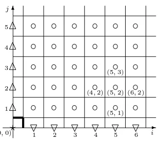
Figure 1 depicts this initial set-up on the first quadrant Z2+ of the integer plane. A ⋆ marks
(0,0), ▽’s mark positions (i, 0), i ≥ 1, △’s positions (0, j), j ≥ 1, and interior points (i, j), i, j≥1 are marked with ◦’s. The coordinates of a few points around (5,2) have been labeled. For a point (i, j)∈Z2+, let Πij be the set of directed paths
π ={(0,0) = (p0, q0)→(p1, q1)→ · · · →(pi+j, qi+j) = (i, j)} (2.1)
with up-right steps
(pl+1, ql+1)−(pl, ql) = (1,0) or (0,1) (2.2)
along the coordinate directions. Define thelast passage time of the point (i, j) as
Gij = max π∈Πij
X
(p,q)∈π
Gsatisfies the recurrence
Gij = (G{i−1}j∨Gi{j−1}) +ωij (i, j ≥0) (2.3)
(with formally assumingG{−1}j = Gi{−1} = 0). A common interpretation is that this models
a growing cluster on the first quadrant that starts from a seed at the origin (bounded by the thickset line in Figure 1). The value ωij is the time it takes to occupy point (i, j) after its
neighbors to the left and below have become occupied, with the interpretation that a boundary point needs only one occupied neighbor. ThenGij is the time when (i, j) becomes occupied, or
joins the growing cluster. The occupied region at time t≥0 is the set
A(t) ={(i, j) ∈Z2+ : Gij ≤t}. (2.4)
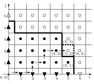
Figure 2 shows a possible later situation. Occupied points are denoted by solidly colored symbols, the occupied cluster is bounded by the thickset line, and the arrows mark an admissible pathπ from (0,0) to (5,2). If G5,2 is the smallest among G0,5, G1,4, G5,2 and G6,0, then (5,2) is the
next point added to the cluster, as suggested by the dashed lines around the (5,2) square. To create a model of random evolution, we pick a real number 0< ̺ <1 and take the variables
{ωij} mutually independent with the following marginal distributions:
ω00= 0, where the ⋆ is,
ωi0 ∼Exp(1−̺), i≥1, where the▽’s are,
ω0j ∼Exp(̺), j≥1, where the △’s are,
ωij ∼Exp(1), i, j≥1, where the ◦’s are.
(2.5)
✲ ✻
⋆ ▽ ▽ ▽ ▽ ▽ ▽
△ △ △ △ △
◦ ◦ ◦ ◦ ◦ ◦
◦ ◦ ◦ ◦ ◦ ◦
◦ ◦ ◦ ◦ ◦ ◦
◦ ◦ ◦ ◦ ◦ ◦
◦ ◦ ◦ ◦ ◦ ◦
(0,0) i
j
1 2 3 4 5 6 1
2 3 4 5
(5,2)
(5,1) (5,3)
(4,2) (6,2)
Figure 1: The initial situation
✲
Figure 2: A possible later situation
Once the parameter̺ has been picked we denote the last-passage time of point (m, n) byG̺mn.
In order to see interesting behavior we follow the last-passage time along the ray defined by
(m(t), n(t)) = (⌊(1−̺)2t⌋,⌊̺2t⌋) (2.6)
as t → ∞. In Section 3.4 we give a heuristic justification for this choice. It represents the characteristic speed of the macroscopic equation of the system. Let us abbreviate
G̺(t) =G̺ ⌊(1−̺)2t⌋,⌊̺2t⌋.
Once we have proved that all horizontal and vertical increments of G-values are distributed exponentially like the boundary increments, we see that
E(G̺(t)) = ⌊(1−̺)
2t⌋
1−̺ + ⌊̺2t⌋
̺ . The first result is the order of the variance.
Theorem 2.1. With 0< ̺ <1 and independent {ωij} distributed as in (2.5),
We emphasize here that our results do not imply a similar statement for the particle flux variance, nor for the position of the second class particle.
For given (m, n) there is almost surely a unique pathπbthat maximizes the passage time to (m, n), due to the continuity of the distribution of{ωij}. Theexit pointofbπ is the last boundary point
on the path. If (pl, ql) is the exit point for the path in (2.1), then eitherp0 =p1 =· · ·=pl = 0
orq0 =q1 =· · ·=ql= 0, andpk, qk≥1 for allk > l. To distinguish between exits via thei- and
j-axis, we introduce a non-zero integer-valued random variable Z such that if Z > 0 then the exit point is (p|Z|, q|Z|) = (Z,0), while if Z <0 then the exit point is (p|Z|, q|Z|) = (0,−Z). For the sake of convenience we abuse language and call the variable Z also the “exit point.” Z̺(t) denotes the exit point of the maximal path to the point (m(t), n(t)) in (2.6) with boundary condition parameter̺. Transpositionωij 7→ωjiof the array shows thatZ̺(t) and−Z1−̺(t) are
Theorem 2.2. Given 0< ̺ <1 and independent {ωij} distributed as in (2.5).
(a) Fort0 >0 there exists a finite constant C=C(t0, ̺) such that, for all a >0 and t≥t0,
P{Z̺(t)≥at2/3} ≤Ca−3.
(b) Givenε >0, we can choose a δ >0 small enough so that for all large enough t
P{1≤Z̺(t)≤δt2/3} ≤ε.
Competition interface. In (6; 7) Ferrari, Martin and Pimentel introduced thecompetition interfacein the last-passage picture. This is a pathk7→ϕk ∈Z2+(k∈Z+), defined as a function
of {Gij}: firstϕ0 = (0,0), and then for k≥0
ϕk+1 =
(
ϕk+ (1,0) ifG(ϕk+ (1,0))< G(ϕk+ (0,1)),
ϕk+ (0,1) ifG(ϕk+ (1,0))> G(ϕk+ (0,1)).
(2.7)
In other words,ϕtakes up-right steps, always choosing the smaller of the two possibleG-values. The term “competition interface” is justified by the following picture. Instead of having the unit squares centered at the integer points as in Figure 1, draw the squares so that their corners coincide with integer points. Label the squares by their northeast corners, so that the square (i−1, i]×(j−1, j] is labeled the (i, j)-square. Regard the last-passage time Gij as the time
when the (i, j)-square becomes occupied. Color the square (0,0) white. Every other square gets either a red or a blue color: squares to the left and above the pathϕare colored red, and squares to the right and below ϕ blue. Then the red squares are those whose maximal path bπ passes through (0,1), while the blue squares are those whose maximal path πb passes through (1,0). These can be regarded as two competing “infections” on the (i, j)-plane, and ϕ is the interface between them.
The competition interface represents the evolution of a second-class particle, and macroscopically it follows the characteristics. This was one of the main points for (7). In the present setting the competition interface is the time reversal of the maximal pathπb, as we explain more precisely in Section 4 below. This connection allows us to establish the order of the transversal fluctuations of the competition interface in the equilibrium setting. To put this in precise notation, we introduce
v(n) = inf{i : (i, n) =ϕk for somek≥0} (2.8)
and
w(m) = inf{j : (m, j) =ϕk for somek≥0}
with the usual convention inf∅ = ∞. In other words, (v(n), n) is the leftmost point of the competition interface on the horizontal linej =n, while (m, w(m)) is the lowest such point on the vertical linei=m. They are connected by the implication
v(n)≥m =⇒ w(m)< n (2.9)
Givenm and n, let
Z∗̺= [m−v(n)]+−[n−w(m)]+ (2.10) denote the signed distance from the point (m, n) to the point where ϕk first hits either of the
lines j = n (Z∗̺ > 0) or i= m (Z∗̺ < 0). Precisely one of the two terms contributes to the difference. When we let m = m(t) and n = n(t) according to (2.6), we have the t-dependent version Z∗̺(t). Time reversal will show that in distribution Z∗̺(t) is equal to Z̺(t). (The
notationZ∗ is used in anticipation of this time reversal connection.) Consequently
Corollary 2.3. Theorem 2.2 is true word for word when Z̺(t) is replaced by Z∗̺(t).
2.2 Results for the rarefaction fan
We now partially generalize the previous results to arbitrary boundary conditions that are bounded by the equilibrium boundary conditions of (2.5). Let{ωij} be distributed as in (2.5).
Let {ωˆij} be another array defined on the same probability space such that ˆω00= 0, ˆωij =ωij
fori, j≥1, and
ˆ
ωi0 ≤ωi0 and ωˆ0j ≤ω0j ∀i, j≥1. (2.11)
In particular, ˆωi0 = ˆω0j = 0 is admissible here. Sections 3.2 and 3.4 below explain how these
boundary conditions can represent the so-called rarefaction fan situation of simple exclusion and cover all the characteristic directions contained within the fan.
Let ˆG(t) denote the weight of the maximal path to (m, n) of (2.6), using the{ωˆij}array.
Theorem 2.4. Fix 0< α <1. There exists a constant C=C(α, ̺) such that for all t≥1 and a >0,
P{|Gˆ(t)−t|> at1/3} ≤Ca−3α/2.
As a last result we show that even with these general boundary conditions, a maximizing path does not fluctuate more than t2/3 around the diagonal of the rectangle. Define ˆZl(t) as the
i-coordinate of the right-most point on the horizontal linej=l of the right-most maximal path to (m, n), and ˆYl(t) as the i-coordinate of the left-most point on the horizontal line j=l of the
left-most maximal path to (m, n). (In this general setting we no longer necessarily have a unique maximizing path because we have not ruled out a dependence of {ωˆi0,ωˆ0j} on{ωˆij}i,j≥1.)
Theorem 2.5. For all 0< α <1 there exists C =C(α, ̺), such that for all a >0, s≤t with t≥1 and(k, l) = ((1−̺)2s,̺2s),
P{Zˆl(t)≥k+at2/3} ≤Ca−3α and P{Yˆl(t)≤k−at2/3} ≤Ca−3α.
3
Particle systems and queues
The proofs in our paper will only use the last-passage description of the model. However, we would like to point out several other pictures one can attach to the last-passage model. An immediate one is the totally asymmetric simple exclusion process (TASEP). The boundary conditions (2.5) of the last-passage model correspond to TASEP in equilibrium, as seen by a “typical” particle right after its jump. We also briefly discuss queues, and an augmentation of
3.1 The totally asymmetric simple exclusion process
This process describes particles that jump unit steps to the right on the integer latticeZ, subject to the exclusion rule that permits at most one particle per site. The state of the process is a
{0,1}-valued sequence eη = {ηex}x∈Z, with the interpretation that ηex = 1 means that site x is
occupied by a particle, andηex= 0 that xis vacant. The dynamics of the process are such that
each (1,0) pair in the state becomes a (0,1) pair at rate 1, independently of the rest of the state. In other words, each particle jumps to a vacant site on its right at rate 1, independently of other particles. The extreme points of the set of spatially translation-invariant equilibrium distributions of this process are the Bernoulli(̺) distributions ν̺ indexed by particle density 0≤̺≤1. Under ν̺ the occupation variables{eηx}are i.i.d. with mean E̺(eηx) =̺.
The Palm distribution of a particle system describes the equilibrium distribution as seen from a “typical” particle. For a functionf ofeη, the Palm-expectation is
b
E̺(f(eη)) = E
̺(f(eη)·ηe
0)
E̺(ηe
0)
in terms of the equilibrium expectation, see e.g. Port and Stone (12). Due to ηex ∈ {0,1}, for
TASEP the Palm distribution is the original Bernoulli(̺)-equilibrium conditioned onηe0 = 1.
Theorem 3.1(Burke). Let eη be a totally asymmetric simple exclusion process started from the Palm distribution (i.e. a particle at the origin, Bernoulli measure elsewhere). Then the position of the particle started at the origin is marginally a Poisson process with jump rate 1−̺.
The theorem follows from considering the inter-particle distances as M/M/1 queues. Each of these distances is geometrically distributed, which is the stationary distribution for the corre-sponding queue. Departure processes from these queues, which correspond to TASEP particle jumps, are marginally Poisson due to Burke’s Theorem for queues, see e.g. Br´emaud (2) for details. The Palm distribution is important in this argument, as selecting a “typical” TASEP-particle assures that the inter-TASEP-particle distances (or the lengths of the queues) are geometrically distributed. For instance, the first particle to the left of the origin in an ordinary Bernoulli equilibrium will not see a geometric distance to the next particle on its right.
Shortly we will explain how the boundary conditions (2.5) correspond to TASEP started from Bernoulli(̺) measure, conditioned on eη0(0) = 0 and
e
η1(0) = 1, i.e. a hole at the origin and a particle at site one initially. It will be
conve-nient to give all particles and holes labels that they retain as they jump (particles to the right, holes to the left). The particle initially at site one is labeled P0, and the hole initially at the
origin is labeled H0. After this, all particles are labeled with integersfrom right to left, and all
holes from left to right. The position of particle Pj at time t is Pj(t), and the position of hole
Hi at timet isHi(t). Thus initially
· · ·< P3(0)< P2(0)< P1(0)< H0(0) = 0
<1 =P0(0)< H1(0)< H2(0)< H3(0)<· · ·
Since particles never jump over each other,Pj+1(t)< Pj(t) holds at all times t≥0, and by the
same token alsoHi(t)< Hi+1(t).
Corollary 3.2. Marginally, P0(t)−1 and −H0(t) are two independent Poisson processes with
respective jump rates1−̺ and ̺.
Proof. The evolution of P0(t) depends only on the initial configuration
{ηex(0)}x>1 and the Poisson clocks governing the jumps over the edges {x → x + 1}x≥1.
The evolution of H0(t) depends only on the initial configuration {ηex(0)}x<0 and the Poisson
clocks governing the jumps over the edges {x → x + 1}x<0. Hence P0(t) and H0(t) are
independent. Moreover, {ηex(0)}x>1, x<0 is Bernoulli(̺) distributed, just like in the Palm
distribution. Hence Burke’s Theorem applies toP0(t). As for H0(t), notice that 1−eη(t), with
1x ≡ 1, is a TASEP with holes and particles interchanged and particles jumping to the left. Hence Burke’s Theorem applies to−H0(t).
Now we can state the precise connection with the last-passage model. Fori, j≥0 let Tij denote
the time when particlePj and holeHi exchange places, withT00= 0. Then
the processes{Gij}i,j≥0 and{Tij}i,j≥0 are equal in distribution.
For the marginal distributions on the i- and j-axes we see the truth of the statement from Corollary 3.2. More generally, we can compare the growing cluster
C(t) ={(i, j) ∈Z2+:Tij ≤t}
with A(t) defined by (2.4), and observe that they are countable state Markov chains with the same initial state and identical bounded jump rates.
Since each particle jump corresponds to exchanging places with a particular hole, one can deduce that at time Tij,
Pj(Tij) =i−j+ 1 and Hi(Tij) =i−j. (3.1)
By the queuing interpretation of the TASEP, we represent particles as servers, and the holes between Pj and Pj−1 as customers in the queue of server j. Then the occupation of the
last-passage point (i, j) is the same event as the completion of the service of customer i by server j. This infinite system of queues is equivalent to a constant rate totally asymmetric zero range process.
3.2 The rarefaction fan
The classical rarefaction fan initial condition for TASEP is constructed with two densitiesλℓ>
λr. Initially particles to the left of the origin obey Bernoulliλℓdistributions, and particles to the
right of the origin follow Bernoulliλr distributions. Of interest here is the behavior of a
second-class particle or the competition interface, and we refer the reader to articles (5; 7; 6; 11; 16) Following the development of the previous section, condition this initial measure on having a hole H0 at 0, and a particle P0 at 1. Then as observed earlier, H0 jumps to the left according
to a Poisson(λℓ) process, whileP0 jumps to the right according to a Poisson(1−λr) process. To
represent this situation in the last-passage picture, choose boundary weights{ωˆi0}i.i.d. Exp(1−
λr), and{ωˆ0j}i.i.d. Exp(λℓ), corresponding to the waiting times ofH0andP0. Supposeλℓ> ̺ >
λr andω is the̺-equilibrium boundary condition defined by (2.5). Then we have the stochastic
domination ωi0 ≥ ωˆi0 and ω0j ≥ ωˆ0j, and we can realize these inequalities by coupling the
3.3 A deposition model
In this section we describe a deposition model that gives a direct graphical connection between the TASEP and the last-passage percolation. This point of view is not needed for the later proofs, hence we only give a brief explanation.
✲
We start by tilting the j-axis and all the vertical columns of Figure 1 by 45 degrees, resulting in Figure 3. This picture represents the same initial situation as Figure 1, but note that now the j-coordinates must be read in the direction տ. (As before, some squares are labeled with their (i, j)-coordinates.) Thei−j tilted coordinate system is embedded in an x−h orthogonal system.
Figure 4: A possible move at a later time
the boundary of the squares belonging to A(t) of (2.4). Whenever it makes sense, the height hx of a column x is defined as the h-coordinate (i.e. the vertical height) of the thickset line
above the edge [x, x+ 1] on the x-axis. Define the increments ηx =hx−1−hx and notice that,
whenever defined,ηx∈ {0,1} due to the tilting we made. The last passage rules, converted for
this picture, tell us that occupation of a new square happens at rate one unless it would violate ηx∈ {0,1}for somex. Moreover, one can read that the occupation of a square (i, j) is the same
event as the pair (ηi−j, ηi−j+1) changing from (1,0) to (0,1). Comparing this to (3.1) leads us
to the conclusion that ηx, whenever defined, is the occupation variable of the simple exclusion
process that corresponds to the last passage model. This way one can also conveniently include the particles (ηx = 1) and holes (ηx = 0) on thex-axis, as seen on the figures. Notice also that
the time-incrementhx(t)−hx(0) is the cumulative particle current across the bond [x, x+ 1].
3.4 The characteristics
One-dimensional conservative particle systems have the conservation law
∂t̺(t, x) +∂xf(̺(t, x)) = 0 (3.2)
under the Eulerian hydrodynamic scaling, where̺(t, x) is the expected particle number per site and f(̺(t, x)) is the macroscopic particle flux around the rescaled position x at the rescaled time t, see e.g. (10) for details. Disturbances of the solution propagate with the characteristic speed f′(̺). The macroscopic particle flux for TASEP is f(̺) = ̺(1 −̺), and consequently the characteristic speed isf′(̺) = 1−2̺. Thus the characteristic curve started at the origin is t7→(1−2̺)t. To identify the point (m, n) in the last-passage picture that corresponds to this curve, we reason approximately. Namely, we look form and nsuch that hole Hm and particle
Pn interchange positions at around time t and the characteristic position (1−2̺)t. By time t,
that particlePnhas jumped over approximately (1−̺)tsites due to Burke’s Theorem. Hence at
time zero, Pn is approximately at position (1−2̺)t−(1−̺)t=−̺t. Since the particle density
is̺, the particle labels around this position aren≈̺2tat time zero. Similarly, holes travel at a speed −̺, so holeHm starts from approximately (1−2̺)t+̺t. They have density 1−̺, which
indicatesm ≈(1−̺)2t. Thus we are led to consider the point (m, n) = (⌊(1−̺)2t⌋,⌊̺2t⌋) as
done in (2.6).
In the rarefaction fan situation with initial density
̺(0, x) = (
λℓ, x <0
λr, x >0
withλℓ> λr
all curvest7→(1−2̺)tfor̺∈[λr, λℓ] are characteristics emanating from the origin. With this
initial density the entropy solution of the conservation law (3.2) is
̺(t, x) =
λℓ, x <(1−2λℓ)t
1
2 −2xt, (1−2λℓ)t < x <(1−2λr)t
λr, x >(1−2λr)t.
For given densities λℓ > λr and Bernoulli initial occupations, we can take any ̺ ∈ [λr, λℓ]
A macroscopic calculation utilizing ̺(t, x) and the fluxf(̺(t, x)) concludes that again, roughly speaking, particle̺2tmeets hole (1−̺)2tat point (1−2̺)tat timet, for each̺∈[λr, λℓ]. Thus
the endpoints (m, n) = (⌊(1−̺)2t⌋,⌊̺2t⌋) that are possible in Theorem 2.4 cover the entire
range of characteristic directions for givenλℓ > λr.
4
Preliminaries
We turn to establish some basic facts and tools. First an extension of Corollary 3.2 to show that Burke’s Theorem holds for every hole and particle in the last-passage picture. Define
Iij : =Gij−G{i−1}j fori≥1, j≥0, and
Jij : =Gij−Gi{j−1} fori≥0, j≥1.
(4.1)
Iij is the time it takes for particlePj to jump again after its jump to sitei−j. Jij is the time it
takes for holeHi to jump again after its jump to sitei−j+ 1. Applying the last passage rules
(2.3) shows
Iij =Gij −G{i−1}j
= (G{i−1}j∨Gi{j−1}) +ωij−G{i−1}{j−1}
−(G{i−1}j −G{i−1}{j−1})
= (J{i−1}j∨Ii{j−1}) +ωij−J{i−1}j
= (Ii{j−1}−J{i−1}j)++ωij.
(4.2)
Similarly,
Jij = (J{i−1}j−Ii{j−1})++ωij. (4.3)
For later use, we define
X{i−1}{j−1} =Ii{j−1}∧J{i−1}j. (4.4)
Lemma 4.1. Fix i, j ≥ 1. If Ii{j−1} and J{i−1}j are independent exponentials with respective
parameters 1−̺ and ̺, then Iij, Jij, and X{i−1}{j−1} are jointly independent exponentials with
respective parameters 1−̺, ̺, and1.
Proof. As the variablesIi{j−1},J{i−1}j andωij are independent, we use (4.2), (4.3) and (4.4) to
write the joint moment generating function as
MIij, Jij, X{i−1}{j−1}(s, t, u) :=Ee
sIij+tJij+uX{i−1}{j−1}
=Ees(Ii{j−1}−J{i−1}j)++t(J{i−1}j−Ii{j−1})++u(Ii{j−1}∧J{i−1}j)·Ee(s+t)ωij
where it is defined. Then, with the assumption of the lemma and the definition ofωij, elementary
calculations show
MIij, Jij, X{i−1}{j−1}(s, t, u) =
̺·(1−̺)
Let Σ be the set of doubly-infinite down-right paths in the first quadrant of the (i, j)-coordinate system. In terms of the sequence of points visited a path σ∈Σ is given by
σ ={· · · →(p−1, q−1)→(p0, q0)→(p1, q1)→ · · · →(pl, ql)→. . .}
with all pl, ql≥0 and steps
(pl+1, ql+1)−(pl, ql) =
(
(1,0) (direction →in Figure 1), or (0,−1) (direction ↓in Figure 1).
The interior of the set enclosed byσ is defined by
B(σ) ={(i, j) : 0≤i < pl, 0≤j < ql for some (pl, ql)∈σ}.
The last-passage time increments along σ are the variables
Zl(σ) =Gpl+1ql+1−Gplql=
(
Ipl+1ql+1, if (pl+1, ql+1)−(pl, ql) = (1,0), Jplql, if (pl+1, ql+1)−(pl, ql) = (0,−1),
forl∈Z. We admit the possibility thatσ is the union of the i- andj-coordinate axes, in which caseB(σ) is empty.
Lemma 4.2. For any σ ∈Σ, the random variables
{Xij : (i, j)∈ B(σ)}, {Zl(σ) :l∈Z} (4.5)
are mutually independent,I’s withExp(1−̺),J’s withExp(̺), andX’s withExp(1)distribution.
Proof. We first consider the countable set of paths that join the j-axis to the i-axis, in other words those for which there exist finite n0 < n1 such that pn = 0 for n ≤ n0 and qn = 0 for
n ≥ n1. For these paths we argue by induction on B(σ). When B(σ) is the empty set, the
statement reduces to the independence of ω-values on the i- and j-axes which is part of the set-up.
Now given an arbitrary σ ∈ Σ that connects the j- and the i-axes, consider a growth corner
(i, j) for B(σ), by which we mean that for some indexl∈Z,
(pl−1, ql−1),(pl, ql),(pl+1, ql+1) = (i, j+ 1),(i, j),(i+ 1, j).
A new valid eσ∈Σ can be produced by replacing the above points with
(pel−1,eql−1),(epl,qel),(pel+1,qel+1) = (i, j+ 1),(i+ 1, j+ 1),(i+ 1, j)
and nowB(σe) =B(σ)∪ {(i, j)}.
The change inflicted on the set of random variables (4.5) is that
{I{i+1}j, Ji{j+1}} (4.6)
has been replaced by
By (4.2)–(4.3) variables (4.7) are determined by (4.6) andω{i+1}{j+1}. If we assume inductively
thatσsatisfies the conclusion we seek, then so doeseσby Lemma 4.1 and because in the situation under considerationω{i+1}{j+1} is independent of the variables in (4.5).
For an arbitrary σ the statement follows because the independence of the random variables in (4.5) follows from independence of finite subcollections. Consider any squareR ={0≤i, j≤M} large enough so that the corner (M, M) lies outside σ∪ B(σ). Then theX- andZ(σ)-variables associated to σ that lie inR are a subset of the variables of a certain pathσe that goes through the points (0, M) and (M,0). Thus the variables in (4.5) that lie inside an arbitrarily large square are independent.
By applying Lemma 4.2 to a path that contains the horizontal line ql ≡ j we get a version
of Burke’s theorem: particle Pj obeys a Poisson process after time G0j when it “enters the
last-passage picture.” The vertical line pl≡igives the corresponding statement for hole Hi.
Example 2.10.2 of Walrand (17) gives an intuitive understanding of this result. Our initial state corresponds to the situation when particle P0 and hole H0 have just exchanged places in an
equilibrium system of queues. H0 is therefore a customer who has just moved from queue 0 to
queue 1. By that Example, this customer sees an equilibrium system of queues every time he jumps. Similarly, any new customer arriving to the queue of particle P1 sees an equilibrium
queue system in front, so Burke’s theorem extends to the region betweenP0 and H0.
Up-right turns do not have independence: variablesIij and Ji{j+1}, or Jij and I{i+1}j are not
independent.
The same inductive argument with a growing cluster B(σ) proves a result that corresponds to a coupling of two exclusion systemsη and ηewhere the latter has a higher density of particles. However, the lemma is a purely deterministic statement.
Lemma 4.3. Consider two assignments of values {ωij} and {ωeij} that satisfy ω00 = eω00 = 0,
ω0j ≥ωe0j, ωi0 ≤ ωei0, and ωij = ωeij for all i, j ≥ 1. Then all increments satisfy Iij ≤ Ieij and
Jij ≥Jeij.
Proof. One proves by induction that the statement holds for all increments between points in σ∪ B(σ) for those paths σ ∈Σ for which B(σ) is finite. If B(σ) is empty the statement is the assumption made on the ω- and ωe-values on the i- and j-axes. The induction step that adds a growth corner toB(σ) follows from equations (4.2) and (4.3).
4.1 The reversed process.
Fixm >0 and n >0, and define
Hij =Gmn−Gij
for 0 ≤ i ≤ m, 0 ≤ j ≤ n. This is the time needed to “free” the point (i, j) in the reversed process, started from the moment when (m, n) becomes occupied. For 0≤i < mand 0≤j < n,
Hij =−((G{i+1}j−Gmn)∧(Gi{j+1}−Gmn))
+ ((G{i+1}j−Gij)∧(Gi{j+1}−Gij))
with definition (4.4) of the X-variables. Taking this and Lemma 4.2 into account, we see that the H-process is a copy of the original G-process, but with reversed coordinate directions. Precisely speaking, define ω∗
00 = 0, and then for 0 < i ≤ m, 0 < j ≤ n: ωi∗0 = I{m−i+1}n,
ω0∗j =Jm{n−j+1}, andωij∗ =X{m−i}{n−j}. Then{ωij∗ : 0≤i≤m,0≤j≤n}is distributed like {ωij : 0≤i≤m,0≤j≤n} in (2.5), and the process
G∗ij =H{m−i}{n−j} (4.8)
for 0≤i≤m, 0≤j≤nsatisfies
G∗ij = (G∗{i−1}j ∨G∗i{j−1}) +ω∗ij, 0≤i≤m ,0≤j≤n
(with the formal assumption G∗{−1}j = Gi∗{−1} = 0), see (2.3). Thus the pair (G∗, ω∗) has the same distribution as (G, ω) in a fixed rectangle {0 ≤ i≤ m} × {0 ≤ j ≤ n}. Throughout the paper quantities defined in the reversed process will be denoted by a superscript∗, and they will always be equal in distribution to their original forward versions.
4.2 Exit point and competition interface.
For integers x define
Ux̺=G{x+}{x−} =
(Px
i=0ωi0, x≥0
P−x
j=0ω0j, x≤0.
(4.9)
Referring to the two coordinate systems in Figure 3, this is the last-passage time of the point on the (i, j)-axes above point x on the x-axis. This point is on the i-axis if x ≥0 and on the j-axis if x≤0.
Fix integersm≥x+∨1,n≥x−∨1, and define Πx(m, n) as the set of directed pathsπconnecting
(x+∨1, x−∨1) and (m, n) using allowable steps (2.2). Then let
Ax =Ax(m, n) = max π∈Πx(m,n)
X
(p,q)∈π
ωpq (4.10)
be the maximal weight collected by a path from (x+, x−) to (m, n) that immediately exits the axes, and does not count ωx+x−. Notice that A−1=A0 =A1 and this value is the last-passage
time from (1,1) to (m, n) that completely ignores the boundaries, or in other words, sets the boundary valuesωi0 and ω0j equal to zero.
By the continuity of the exponential distribution there is an a.s. unique path bπ from (0,0) to (m, n) which collects the maximal weight G̺mn. Earlier we defined the exit point Z̺ ∈ Z to
represent the last point of this path on either thei-axis or the j-axis. Equivalently we can now state thatZ̺is the a.s. unique integer for which
G̺mn=UZ̺̺+AZ̺.
Simply because the maximal pathπbnecessarily goes through either (0,1) or (1,0), Z̺is always nonzero.
of the reversed process follows the maximal path bπ backwards from the corner (m, n), until it hits either the i- or the j-axis. To make a precise statement, let us represent the a.s. unique maximal last-passage path, with exit point Z̺ as defined above, as
b
π ={(0,0) =bπ0 →bπ1→ · · · →πb|Z̺|→ · · · →bπm+n= (m, n)},
where{bπ|Z̺|+1 → · · · →πbm+n}is the portion of the path that resides in the interior{1, . . . , m}×
{1, . . . , n}.
Lemma 4.4. Let ϕ∗ be the competition interface constructed for the process G∗ defined by (4.8). Thenϕ∗
k = (m, n)−bπm+n−k for 0≤k≤m+n− |Z̺|.
Proof. Starting frombπm+n= (m, n), the maximal pathπbcan be constructed backwards step by
step by always moving to the maximizing point of the right-hand side of (2.3). This is the same as constructing the competition interface for the reversed process G∗ by (2.7). Since G∗ is not constructed outside the rectangle{0, . . . , m}×{0, . . . , n}, we cannot assert what the competition interface does after the point
ϕ∗m+n−|Z̺|=bπ|Z̺|=
(
(Z̺,0) if Z̺>0
(0,−Z̺) if Z̺<0.
Notice that, due to this lemma,Z∗̺defined in (2.10) is indeedZ̺defined in the reversed process,
which justifies the argument following (2.10).
The competition interface bounds the regions where the boundary conditions on the axes are felt. From this we can get useful bounds between last-passage times under different boundary conditions. This is the last-passage model equivalent of the common use of second-class particles to control discrepancies between coupled interacting particle systems. In the next lemma, the superscriptWrepresents the west boundary (j-axis) of the (i, j)-plane. Remember that (v(n), n) is the left-most point of the competition interface on the horizontal linej=ncomputed in terms of the G-process (see (2.8)).
Lemma 4.5. LetGW=0 be the last-passage times of a system where we set ω0j = 0 for allj≥1.
Then for v(n)< m1< m2,
A0(m2, n)−A0(m1, n)≤GW=0(m2, n)−GW=0(m1, n)
=G(m2, n)−G(m1, n).
Proof. The first inequality is a consequence of Lemma 4.3, because computing A0 is the same
as computingG with all boundary values ωi0 =ω0j = 0 (and in fact this inequality is valid for
all m1 < m2.) The equality G(m, n) =GW=0(m, n) form > v(n) follows because the maximal
path bπ for G(m, n) goes through (1,0) and hence does not see the boundary values ω0j. Thus
this same pathbπ is maximal forGW=0(m, n) too.
If we set ωi0 = 0 (the south boundary denoted by S) instead, we get this statement: for
0≤m1 < m2 ≤v(n),
A0(m2, n)−A0(m1, n)≥GS=0(m2, n)−GS=0(m1, n)
=G(m2, n)−G(m1, n).
4.3 A coupling on the i-axis
Let 1> λ > ̺ >0. As a common realization of the exponential weightsωiλ0 of Exp(1−λ) and ωi̺0 of Exp(1−̺) distribution, we write
ωλi0 = 1−̺ 1−λ·ω
̺
i0. (4.12)
We will use this coupling later for different purposes. We will also need
Var(ωiλ0−ω̺i0) =
1−̺ 1−λ−1
2
· 1
(1−̺)2 =
1 1−λ−
1 1−̺
2
.
4.4 Exit point and the variance of the last-passage time
With these preliminaries we can prove the key lemma that links the variance of the last-passage time to the weight collected along the axes.
Lemma 4.6. Fix m, n positive integers. Then
Var(G̺mn) = n ̺2 −
m (1−̺)2 +
2
1−̺ ·E(U
̺ Z̺+)
= m (1−̺)2 −
n ̺2 +
2 ̺ ·E(U
̺ −Z̺−),
(4.13)
where Z̺is the a.s. unique exit point of the maximal path from (0,0) to(m, n).
Proof. We label the total increments along the sides of the rectangle by compass directions:
W =G̺0n−G̺00, N =G̺mn−G̺0n, E =G̺mn−G̺m0, S =G̺m0−G̺00.
AsN and E are independent by Lemma 4.2, we have
Var(G̺mn) =Var(W+N)
=Var(W) +Var(N) + 2Cov(S+E − N,N) =Var(W)−Var(N) + 2Cov(S,N).
(4.14)
We now modify the ω-values in S. Letλ=̺+εand apply (4.12), without changing the other values {ωij :i≥0, j ≥1}. Quantities of the altered last-passage model will be marked with a
superscriptε. In this new process,Sε has a Gamma(m,1−̺−ε) distribution with density
fε(s) =
(1−̺−ε)m·e−(1−̺−ε)s·sm−1 (m−1)!
fors >0, whose ε-derivative is
∂εfε(s) =sfε(s)−
m
Given the sumSε, the joint distribution of{ω
i0}1≤i≤m is independent of the parameterε, hence
the quantityE(Nε| Sε =s) = E(N | S =s) does not depend on ε. Therefore, using (4.15) we
have
∂εE(Nε)
ε=0=∂ε
Z ∞
0
E(N | S=s)fε(s) ds
ε=0
= Z ∞
0
E(N | S=s)·s·f0(s) ds−
m 1−̺
Z ∞
0
E(N | S =s)f0(s) ds
=E(N S)− m
1−̺ ·E(N) =Cov(N,S).
(4.16)
Next we compute the same quantity by a different approach. LetZ andZε be the exit points of the maximal paths to (m, n) in the original and the modified processes, respectively. Similarly, Ux and Uxε are the weights as defined by (4.9) for the two processes. Hence UZ is the weight
collected on theiorj axis by the maximal path of the original process. Then
Nε− N = (Nε− N)·1{Zε=Z}+ (Nε− N)·1{Zε6=Z} = (UZε −UZ)·1{Zε=Z}+ (Nε− N)·1{Zε 6=Z}
= (UZε −UZ) + (Nε− N −UZε +UZ)·1{Zε 6=Z}.
Asω values are only changed on the i-axis, the first term is rewritten as
UZε −UZ =UZε+−UZ+ =
1−̺ 1−̺−ε −1
UZ+ = ε
1−̺−ε·UZ+
by (4.12). We show that the expectation of the second term is o(ε). Note that the increase Nε− N is bounded bySε− S. Hence
E[(Nε− N −UZε +UZ)·1{Zε6=Z}]
≤E[(Nε− N)·1{Zε6=Z}] ≤ E[(Sε− S)·1{Zε6=Z}]
≤ E[(Sε− S)2]12 · P{Zε6=Z}12.
(4.17)
To show that the probability is of the order of ε, notice that the exit point of the maximal path can only differ in the modified process from the one of the original process, if for some Z < k≤m,Uε
k+Ak > UZε +AZ withZ of the original process (see (4.10) for the definition of
Ai). Therefore,
P{Zε 6=Z}=P{Ukε+Ak> UZε +AZ for someZ < k≤m}
=P{Ukε−UZε > AZ−Ak for someZ < k≤m}
=P{Ukε−UZε > AZ−Ak≥Uk−UZ for someZ < k≤m} ≤P{Ukε−Uiε> Ai−Ak≥Uk−Ui for some 0≤i < k≤m}
≤ X
0≤i<k≤m
P{Ukε−Uiε> Ai−Ak≥Uk−Ui}.
We also used the definition ofZ in the third equality, viaAZ+UZ ≥Ak+Uk. Notice thatA’s
we write
SinceUk−Ui has a Gamma distribution, the supremum above isO(ε), which shows the bound
on P{Zε6=Z}. The first factor on the right-hand side of (4.17),
The proof of the first statement is then completed by this display, (4.14) and (4.16), as W and
N are Gamma-distributed by Lemma 4.2. The second statement follows in a similar way, using Cov(W,E). thejaxis. Note that in this coupling, when changing from̺ toλ, we are increasing the weights on thei-axis and decreasing the weights on thej-axis, which clearly implies Z̺≤Zλ. Also, we remain in the stationary situation, so (4.13) remains valid forλ. As U−̺x− is non-increasing in
x, this implies
We substitute this into the second line of (4.13) to get
5
Upper bound
We turn to proving the upper bounds in Theorems 2.1 and 2.2. We have a fixed density̺∈(0,1), and to study the last-passage times G̺ along the characteristic, we define the dimensions of the
last-passage rectangle as
m(t) =(1−̺)2t and n(t) =̺2t (5.1)
with a parametert→ ∞. The quantities Ax,Z andGmnconnected to these indices are denoted
byAx(t),Z(t),G(t). In the proofs we need to consider different boundary conditions (2.5) with
̺replaced byλ. This will be indicated by a superscript. However, the superscriptλonly changes the boundary conditions and not the dimensionsm(t) andn(t), always defined by (5.1) with a fixed ̺. Moreover, we apply the coupling (4.12) on the i-axis andωλ
0j = λ̺ ·ω ̺
0j on the j-axis.
The weights{ωij}i, j≥1 in the interior will not be affected by changes in boundary conditions, so
in particularAx(t) will not either. SinceGλ(t) chooses the maximal path,
Uzλ+Az(t)≤Gλ(t)
for all 1≤z≤m(t) and all densities 0< λ <1. Consequently, for integers u≥0 and densities λ≥̺,
P{Z̺(t)> u}=P{∃z > u : Uz̺+Az(t) =G̺(t)} ≤P{∃z > u : Uz̺−Uzλ+Gλ(t)≥G̺(t)} =P{∃z > u : Uzλ−Uz̺≤Gλ(t)−G̺(t)}
≤P{Uuλ−Uu̺≤Gλ(t)−G̺(t)}.
(5.2)
The last step is justified by λ≥̺ and the coupling (4.12).
To put the subsequent technicalities into context, we give a rough summary of the argument that follows. To get an upper bound forVar(G̺(t)), by Lemma 4.6 it suffices to find an upper bound for the mean of UZ̺̺(t)+. The goal will be to obtain an inequality of the type
P{UZ̺̺(t)+ > y} ≤C t2 y4 ·E(U
̺
Z̺(t)+) + (error terms). (5.3)
This is sufficient to guarantee thatE(UZ̺̺(t)+) does not grow faster thant2/3, provided the error terms can be handled. Informally speaking, here is the logic that produces inequality (5.3). If UZ̺̺(t)+ is too large, then except for a large deviation, it must be thatZ̺(t) is too large. When G̺(t) collects too much weight on the i-axis, we compare it to a λ-system with λ > ̺, as was done in (5.2) above. By choosing λ appropriately we can make E(Uλ
u −Uu̺−Gλ(t) +G̺(t))
We turn to the details of the derivation of the upper bound, beginning with the optimal choice with the help of Lemma 4.2. Some useful identities for future computations:
λu≥̺,
Proof. By Lemma 4.2 and (5.1)
E(Uλu
equals the main term of the bound.
This is easy to check in the form
Since the expression in parentheses is not larger than 1,u/t≤ 34(1−̺)2, and ̺≤λu, it follows
that
Var(Gλu(t))≤Var(G̺(t)) + 4
(1−̺)2 ·u.
Then we proceed with Lemma 4.6 and (5.1):
Var(Gλu(t)−G̺(t))≤2Var(Gλu(t)) + 2Var(G̺(t))
After these preparations, we continue the main argument from (5.2).
account, we write
the statement still holds, modified by a factor of a power of 4/3. Finally, the probability is trivially zero ifu >(1−̺)2t.
Fix a number 0< α <1, and define
y= u
α(1−̺). (5.6)
Lemma 5.6. We have the following large deviations estimate:
Lemma 5.7. There exist finite positive constants C2 =C2(α, ̺) and C3 =C3(α, ̺) such that,
Proof. The first inequality implies the second one by Lemma 4.6 and (5.1). To prove the first one, suppose that there exists a sequence tk ր ∞such that
lim
k for all large k’s, and consequently by the above lemma
Combining Lemma 5.5 and Theorem 5.8 gives a tail bound onZ:
Corollary 5.9. Given any t0 >0 there exists a finite constant C4 =C4(t0, ̺) such that, for all
a >0 and t≥t0,
P{Z̺(t)≥at2/3} ≤C4a−3.
6
Lower bound
The lower bound is a little more subtle than the upper bound for in a sense there is “less room in the estimates.” The objective is to show that UZ̺̺(t)+ genuinely fluctuates on the scale t2/3, and then again Lemma 4.6 translates this into a lower bound onVar(G̺(t)). So the main point
is to prove this lemma:
Lemma 6.1. We have the asymptotics
lim
εց0lim supt→∞
P{0< UZ̺̺(t)+ ≤εt2/3}= 0.
Note that part of the event is the requirementZ̺(t)>0. SinceU̺is a sum of i.i.d. exponentials,
the work lies really in controlling the pointZ̺(t). To make this explicit write
P{0< UZ̺̺(t)+ ≤εt2/3} ≤P{0< Z̺(t)≤δt2/3}+P{U
̺
⌊δt2/3⌋≤εt2/3}.
Givenδ >0, the last probability vanishes ast→ ∞for anyε < δ(1−̺)−1. Thus it remains to show that the first probability on the right can be made arbitrarily small for larget, by choosing a small enough δ.
Let 0 < δ, b < 1. Utilizing the fact that Z̺(t) marks the exit point of the maximal path, we
split this probability into two parts.
P{0< Z̺(t)≤δt2/3}
≤Pn sup
x>δt2/3
Ux̺+Ax(t)< sup
1≤x≤δt2/3
Ux̺+Ax(t)o
≤P n
sup
x>δt2/3
Ux̺+Ax(t)−A1(t)
< bt1/3o (6.1)
+ Pn sup
1≤x≤δt2/3
Ux̺+Ax(t)−A1(t)
> bt1/3o. (6.2)
Next we bound the probabilities (6.1) and (6.2) separately. We abbreviate (m, n) = (1−̺)2t,̺2t throughout this section.
We do not have direct control over the quantityAx(t)−A1(t) that appears in both probabilities
(6.1) and (6.2). As defined in (4.10), these are last passage times that use only the internal weights{ωij :i, j≥1}and thereby are not constrained by the boundary conditions. But we can
influence of the boundary conditions, as shown in Lemma 4.5 and equation (4.11). The location of the competition interface is controlled by Corollary 5.9 which applies toZ∗̺of (2.10) by time reversal (recall discussion before and after Lemma 4.4).
The only impediment appears to be that Lemma 4.5 and equation (4.11) concern a difference A0(m2, n)−A0(m1, n) of two last-passage times emanating from the common point (1,1) but
ending up at different points on the same horizontal line at level n, while we need to treat Ax(t)−A1(t) where the last-passage times emanate from different points (x,1) and (1,1) but
end up at (m, n). However, these situations can be turned into each other by reversing the coordinate directions of the internal weights. The maximal path between two points on the lattice does not depend on which point we declare the starting point and which the ending point.
This argument is made precise in the next lemma which develops a bound for probability (6.2). After that we handle (6.1) with similar reasoning.
Lemma 6.2. Let a, b > 0 be arbitrary positive numbers. There exist finite constants t0 =
t0(a, b, ̺) and C=C(̺) such that, for all t≥t0,
Pn sup
1≤z≤at2/3
Uz̺+Az(t)−A1(t) ≥bt1/3
o
≤Ca3(b−3+b−6).
Proof. The process {Uz̺} depends on the boundary {ωi0}. Pick a version
{ωij}1≤i≤m,1≤j≤n of the interior variables independent of {ωi0}. If we use the reversed
system
{ωeij =ωm−i+1,n−j+1}1≤i≤m,1≤j≤n (6.3)
to computeAz(m, n), then this coincides withA1(m−z+ 1, n) computed with{ωij}. Thus with
this coupling (and some abuse of notation) we can replace Az(m, n)−A1(m, n) with A1(m−
z + 1, n) −A1(m, n). [Note that A1(m, n) is the same for ω and ωe.] Next pick a further
independent version of boundary conditions (2.5) with density λ. Use these and {ωij}i,j≥1 to
compute the last-passage times Gλ, together with a competition interface ϕλ defined by (2.7)
and the projectionsvλ defined by (2.8). Then by (4.11), on the eventvλ(n)≥m,
A1(m, n)−A1(m−z+ 1, n)≥Gλ(m, n)−Gλ(m−z+ 1, n).
Set
Vzλ =Gλ(m, n)−Gλ(m−z, n),
a sum of z i.i.d. Exp(1−λ) variables. Vλ is independent of U̺. Combining these steps we get the bound
P n
sup
1≤z≤at2/3
Uz̺+Az(t)−A1(t)
≥bt1/3o
≤Pvλ(̺2t)<(1−̺)2t +P n
sup
1≤z≤at2/3
(Uz̺−Vzλ−1)≥bt1/3o
(6.4)
Introduce a parameter r >0 whose value will be specified later, and define
For the second probability on the right-hand side of (6.4), define the martingale Mz = Uz̺−
Vzλ−1−E(Uz̺−Vzλ−1), and note that forz≤at2/3,
E(Uz̺−Vzλ−1) = z 1−̺ −
z−1 1−λ =
zrt−1/3 (1−̺)(1−λ)+
1 1−λ
≤ rat
1/3
(1−̺)2 +
1 1−̺.
As long as
b > ra(1−̺)−2+t−1/3(1−̺)−1, (6.6) we get by Doob’s inequality, for anyp≥1,
Pn sup
1≤z≤at2/3
(Uz̺−Vzλ−1)≥bt1/3o
≤Pn sup
1≤z≤at2/3
Mz≥t1/3
b− ra (1−̺)2 −
t−1/3
1−̺ o
≤ C(p)t− p/3
b−ra(1−̺)−2−t−1/3(1−̺)−1pE
|M⌊at2/3⌋|p
≤ C(p, ̺)a p/2
b−ra(1−̺)−2−t−1/3(1−̺)−1p.
(6.7)
Now chooset0 = 43b−3(1−̺)−3. Then fort≥t0 the above bound is dominated by
C(p, ̺)ap/2
3b
4 −(1−ra̺)2 p
which becomes C(p, ̺)a3b−6 once we choose
r= b(1−̺)
2
4a (6.8)
and p= 6, and change the constant C(p, ̺).
For the first probability on the right-hand side of (6.4), introduce the times= (̺/λ)2t. Then
Pvλ(̺2t)<(1−̺)2t =Pvλ(λ2s)<λ2(1−̺)2̺−2s .
Notice that since λ < ̺ here, λ2(1−̺)2̺−2s ≤ (1−λ)2s and so by redefining (2.6) and (2.10) withsand λ, we have that the eventvλ(λ2s)<λ2(1−̺)2̺−2sis equivalent to
Z∗λ(s) = [(1−λ)2s−vλ(λ2s)]+−[λ2s−wλ((1−λ)2s)]+ =(1−λ)2s−vλ(λ2s)
>(1−λ)2s−λ2(1−̺)2̺−2s.
By Z∗λ =d Zλ, we conclude
Pvλ(̺2t)<(1−̺)2t
Utilizing the definitions (6.5) and (6.8) ofλandr, one can check that by increasingt0 =t0(a, b, ̺)
if necessary, one can guarantee that fort≥t0 there exists a constantC =C(̺) such that
(1−λ)2s−λ2(1−̺)2̺−2s≥Crs2/3.
Combining this with Corollary 5.9 and definition (6.8) ofr we get the bound
Pvλ(̺2t)<(1−̺)2t ≤PZλ(s)> Crs2/3 ≤Cr−3 ≤C(a/b)3.
Returning to (6.4) to combine all the bounds, we have
P
Completion of the proof of Lemma 6.1. By Lemma 6.2 the probability (6.2) is bounded by Cδ3(b−3+b−6). Bound the probability (6.1) by
where, following the example of the previous proof, we have introduced a new density, this time
λ=̺+rt−1/3,
and then used the reversal trick of equation (6.3) and Lemma 4.5 to deduce
Ax(m, n)−A1(m, n)≥Gλ(m−x+ 1, n)−Gλ(m, n)≡ −Vxλ−1≥ −Vxλ,
whereB(·) is standard Brownian motion. The random variable
sup
0≤y≤1
σ(̺)B(y)− ry (1−̺)2
is positive almost surely, so the above probability is less thanη/2 for smallδ andb. This implies (6.12).
The probability in (6.10) is bounded by
Pvλ(⌊̺2t⌋)>⌊(1−̺)2t−t2/3−1⌋
≤Pv1−λ(⌊(1−̺)2t−t2/3−1⌋)<⌊̺2t⌋ ≤Pv1−λ(⌊(1−λ)2s⌋)<⌊λ2s⌋ −qs2/3 =PZ∗1−λ(s)> qs2/3
=PZ1−λ(s)> qs2/3 ≤Cq−3.
Above we first used (2.9) and transposition of the array{ωij}. Because this exchanges the axes,
densityλbecomes 1−λ. Then we definedsby
(1−λ)2s= (1−̺)2t−t2/3−1
and observed that for large enought, the second inequality holds for someq=C(̺)((1−̺)r−̺). We used (2.10) and the distributional identity of Z and Z∗ thereafter. The last inequality is
from Corollary 5.9.
Now givenη >0, chooserlarge enough so thatCq−3< η. Given thisr, chooseδ, bsmall enough
so that (6.12) holds. Finally, shrinkδ further so that Cδ3(b−3+b−6)< η (shrinkingδ does not violate (6.12)). To summarize, we have shown that, given η >0, if δ is small enough, then for all large t
P{1≤Z̺(t)≤δt2/3} ≤3η. (6.13) This concludes the proof of the lemma.
Via transpositions we get Lemma 6.1 also for thej-axis:
Corollary 6.3. We have the asymptotics
lim
εց0lim supt→∞ P{0< U ̺
−Z̺(t)− ≤εt2/3}= 0.
Proof. Let{ωij}be an initial assignment with density̺. Letωeij =ωji be the transposed array,
which is an initial assignment with density 1−̺. Under transposition the (1−̺)2t×̺2t
rectangle has become ̺2t×(1−̺)2t, the correct characteristic dimensions for density 1−
̺. Since transposition exchanges the coordinate axes, after transposition UZ̺̺(t)+ has become U1−̺
−Z1−̺(t)−, and so these two random variables have the same distribution. The corollary is now
(6.13) proves part (b) of Theorem 2.2. The theorem below gives the lower bound for Theorem 2.1 and thereby completes its proof.
Theorem 6.4.
lim inf
t→∞
E(UZ̺̺(t)+)
t2/3 >0, and lim inft→∞
Var(G̺(t)) t2/3 >0.
Proof. Suppose there exists a density̺and a sequencetk→ ∞such thattk−2/3Var(G̺(tk))→0.
Then by Lemma 4.6
E(UZ̺̺(t k)+)
t2k/3 →0 and
E(U̺
−Z̺(t k)−)
t2k/3 →0. From this and Markov’s inequality
P{UZ̺̺(t
k)+ > εt
2/3
k } →0 and P{U ̺ −Z̺(t
k)−> εt
2/3
k } →0
for everyε >0. This together with Lemma 6.1 and Corollary 6.3 implies
P{UZ̺̺(tk)+ >0} →0 and P{U
̺
−Z̺(tk)−>0} →0.
But these statements imply that
P{Z̺(tk)>0} →0 and P{Z̺(tk)<0} →0,
which is a contradiction since these two probabilities add up to 1 for each fixedtk. This proves
the second claim of the theorem.
The first claim follows because it is equivalent to the second.
7
Rarefaction boundary conditions
In this section we prove results on the longitudinal and transversal fluctuations of a maximal path under more general boundary conditions. Abbreviate as before
(m, n) = (1−̺)2t,̺2t.
We start by studyingA0(t) =A0(m, n), the length of the maximal path to (m, n) when there are
no weights on the axes, and we will show that it has fluctuations of the order t1/3. We still use
the boundary conditions (2.5), so that we have coupledA0(t) andG̺(t). We first need another
version of Lemma 6.2 to make it applicable for all t≥1.
Lemma 7.1. Fix 0< α <1. There exists a constant C=C(α, ̺) such that, for eacht≥1and b≥C,
P{G̺(t)−A0(t)≥bt1/3} ≤Cb−3α/2.
Proof. Note that
P{G̺(t)−A0(t)≥bt1/3}
≤P{ sup
|z|≤at2/3
Uz̺(t) +Az(t)−A0(t)≥bt1/3}
+P{ sup
|z|≤at2/3
Uz̺(t) +Az(t)6=G̺(t)}.
The last term of (7.1) can easily be dealt with using Corollary 5.9: there exists aC =C(̺) such that
P sup
|z|≤at2/3
Uz̺(t) +Az(t)
6
=G̺(t) ≤P{Z̺(t)≥at2/3}
+P{Z̺(t)≤ −at2/3} ≤Ca−3.
(7.2)
For the first term of (7.1) we will use the results from the proof of Lemma 6.2. We split the range ofz into [1, at2/3] and [−1,−at2/3] and consider for now only the first part. Define
λ=̺−rt−1/3.
We can use (6.4) and (6.7), where we choose a = bα/2, p = 2, and r = bα/2. Choose C =
C(α, ̺) > 0 large enough so that for b ≥ C (6.6) is satisfied and the denominator of the last bound in (6.7) is at leastb/2. Then we can claim that, for allb≥C and t≥1,
P sup
1≤z≤at2/3
Uz̺(t) +Az(t)−A0(t)≥bt1/3
≤Pvλ(̺2t)<(1−̺)2t +Cbα/2−2.
(7.3)
From (6.9) we get withs= (̺/λ)2t
Pvλ(̺2t)<(1−̺)2t =PZλ(s)>(1−λ)2s−λ2(1−̺)2̺−2s .
Now we continue differently than in Lemma 6.2 so thattis not forced to be large. An elementary calculation yields
(1−λ)2s−λ2(1−̺)2̺−2s≥21−̺ ̺ rs
2/3+2̺−1
̺2 r 2s1/3
−1.
We want to write down conditions under which the right-hand side above is at least δrs2/3 for some constant δ and all s ≥ 1. First increase the above constant C = C(α, ̺) so that if b=r2/α ≥C, then
1−̺ ̺ rs
2/3−1≥ 1−̺
2̺ rs
2/3 for all s≥1.
Then choose η =η(α, ̺) > 0 small enough such that wheneverb ∈[C, ηt2/(3α)] (in this case r is small enough compared tot1/3, but notice that the interval might as well be empty whentis
small),
1−̺ ̺ rs
2/3
≥ −2̺̺−2 1r2s1/3.
This last condition is vacuously true if̺≥1/2.
Now we have forC≤b≤ηt2/(3α) and withδ = (1−̺)/(2̺),
(1−λ)2s−λ2(1−̺)2̺−2s≥δrs2/3 for all s≥1.
If we combine this with (7.3) and Corollary 5.9, we can state that for all C ≤b≤ηt2/(3α) and t≥1,
P{ sup
1≤z≤at2/3