Full Terms & Conditions of access and use can be found at
http://www.tandfonline.com/action/journalInformation?journalCode=ubes20
Download by: [Universitas Maritim Raja Ali Haji], [UNIVERSITAS MARITIM RAJA ALI HAJI
TANJUNGPINANG, KEPULAUAN RIAU] Date: 11 January 2016, At: 20:49
Journal of Business & Economic Statistics
ISSN: 0735-0015 (Print) 1537-2707 (Online) Journal homepage: http://www.tandfonline.com/loi/ubes20
Conditional Euro Area Sovereign Default Risk
André Lucas, Bernd Schwaab & Xin Zhang
To cite this article: André Lucas, Bernd Schwaab & Xin Zhang (2014) Conditional Euro Area Sovereign Default Risk, Journal of Business & Economic Statistics, 32:2, 271-284, DOI: 10.1080/07350015.2013.873540
To link to this article: http://dx.doi.org/10.1080/07350015.2013.873540
Accepted author version posted online: 31 Dec 2013.
Submit your article to this journal
Article views: 594
View related articles
View Crossmark data
Conditional Euro Area Sovereign Default Risk
Andr ´e LUCAS
Faculty of Economics and Business and Tinbergen Institute, VU University Amsterdam, De Boelelaan 1105, 1081 HV Amsterdam, The Netherlands ([email protected])
Bernd SCHWAAB
Financial Research, European Central Bank, Kaiserstrasse 29, 60311 Frankfurt, Germany ([email protected])
Xin ZHANG
Research Division, Sveriges Riksbank, Brunkebergstorg 11, SE 103 37 Stockholm, Sweden ([email protected])
We propose an empirical framework to assess the likelihood of joint and conditional sovereign default from observed CDS prices. Our model is based on a dynamic skewed-tdistribution that captures all salient features of the data, including skewed and heavy-tailed changes in the price of CDS protection against sovereign default, as well as dynamic volatilities and correlations that ensure that uncertainty and risk dependence can increase in times of stress. We apply the framework to euro area sovereign CDS spreads during the euro area debt crisis. Our results reveal significant time-variation in distress dependence and spill-over effects for sovereign default risk. We investigate market perceptions of joint and conditional sovereign risk around announcements of Eurosystem asset purchases programs, and document a strong impact on joint risk.
KEY WORDS: Financial stability; Higher order moments; Sovereign credit risk; Time-varying parameters.
1. INTRODUCTION
In this article we construct a novel empirical framework to as-sess the likelihood of joint and conditional default on credit risky claims, such as government debt issued by euro area countries. This framework allows us to estimate marginal, joint, and con-ditional probabilities of a sovereign credit event from observed prices of credit default swaps (CDS) on sovereign debt. Default is defined as any credit event that would trigger a sovereign CDS contract, such as the nonpayment of principal or interest when it is due, a forced exchange of debt into claims of lower value, a moratorium, or an official repudiation of the debt. Clearly, a risk assessment and monitoring framework is useful for track-ing market perceptions about interacttrack-ing sovereign risks durtrack-ing a debt crisis. However, the current framework should also be useful for market risk measurement of credit risky claims more generally.
Unlike marginal probabilities, conditional probabilities of sovereign default cannot be obtained from raw market data alone. Instead, they require a proper multivariate modeling framework. Our methodology is novel in that our joint and tail probability assessments are derived from a multivariate frame-work based on a dynamic generalized hyperbolic (GH) skewed-t
density that naturally accommodates all relevant empirical fea-tures of the data, such as skewed and heavy-tailed changes in individual country CDS spreads, as well as time variation in their volatilities and dependence. Moreover, the model can easily be calibrated to match current market expectations regarding the marginal probabilities of default as in, for example, Segoviano and Goodhart (2009), Huang, Zhou, and Zhu (2009), and Black et al. (2012).
We make three empirical contributions in addition to introduc-ing a novel non-Gaussian framework for modelintroduc-ing dependent risks. First, we provide estimates of the time variation in euro area joint and conditional sovereign default risk using a pro-posed model and a 10-dimensional dataset of sovereign CDS spreads from January 2008 to February 2013. Using our results, we can investigate market perceptions regarding the conditional probability of a credit event in one country in the euro area given that a credit event occurs in another country. Such an analysis allows inference, for example, on which countries are consid-ered by market participants to be more exposed to certain credit events than others. Our modeling framework also allows us to investigate the presence and severity of spill-overs in the risk of sovereign credit events as perceived by market participants. Specifically, we document spill-overs from the possibility of a credit event in one country to the perceived riskiness of other euro area countries. This suggests that, at least during a severe debt crisis, the cost of debt refinancing in one euro area country can depend on perceived developments in other countries. This, in turn, is consistent with a risk externality from public debt to other countries in a monetary union.
Second, we analyze the extent to which parametric modeling assumptions matter for joint and conditional risk assessments. Perhaps surprisingly, and despite the appeal of price-based joint
© 2014American Statistical Association Journal of Business & Economic Statistics April 2014, Vol. 32, No. 2 DOI:10.1080/07350015.2013.873540 Color versions of one or more of the figures in the article can be found online atwww.tandfonline.com/r/jbes.
271
risk measures to guide policy decisions and to evaluate their impact on credit markets ex post, we are not aware of a detailed investigation of how different parametric assumptions matter for joint and conditional risk assessments. We, therefore, report results based on a dynamic multivariate Gaussian,
symmetric-t, and GH skewed-t(GHST) specification, as well as a GHST copula approach. The distributional assumptions turn out to be most relevant for our conditional assessments, whereas simpler joint default probability estimates are less sensitive to the as-sumed dependence structure. In particular, and much in line with Forbes and Rigobon (2002), we show that it is important to account for the different salient features of the data, such as nonzero tail dependence and skewness, when interpreting esti-mates of time-varying volatilities and increases in correlation in times of stress.
Finally, we provide an in-depth analysis of the impact on sovereign risk of two key policy announcements made during the euro area sovereign debt crisis. First, on May 9, 2010, euro area heads of state announced a rescue package to mitigate sovereign risk conditions and perceived risk contagion in the euro area. The rescue package contained the European Finan-cial Stability Facility (EFSF), a rescue fund. At the same time, the ECB announced an asset purchase program (the Securities Markets Programme, SMP) within which the European Central Bank and 17 euro area national central banks would purchase government bonds in secondary markets. Later, on August 2, 2012, a second asset purchase program was announced (the Outright Monetary Transactions, OMT). The OMT replaced the earlier SMP. We assess joint and conditional sovereign default risk perceptions, as implied by CDS prices, around both policy announcements. For both the May 2010 and August 2012 an-nouncements we find that market perceptions ofjointsovereign default risk have decreased very strongly. In some cases, joint bivariate risks decreased by more than 50% virtually overnight. We show that these strong reductions in joint risk were due to large reductions in marginal risk perceptions, while market per-ceptions ofconditionalsovereign default risk did not decrease at the same time. This suggests that perceived risk interactions remained a concern.
From a (tail) risk perspective, our joint approach is in line with, for example, Acharya et al. (2010) who focused on finan-cial institutions: bad outcomes are much worse if they occur in clusters. What seems manageable in isolation may not be so if the rest of the system is also under stress. While adverse develop-ments in one country’s public finances or banking sectors could perhaps still be handled with the support of other nondistressed countries, the situation becomes more and more problematic if two, three, or more countries would be in distress. Relevant questions regarding joint and conditional sovereign default risk perceptions would be hard if not impossible to answer without an empirical model such as the one proposed in this article.
The use of CDS data to estimate market implied default prob-abilities means that our probability estimates combine physical default probabilities with the price of sovereign default risk. As a result, our risk measures constitute an upper bound for an investor worried about losing money due to joint sovereign defaults. This has to be kept in mind when interpreting the em-pirical results later on. Estimating default probabilities directly from observed defaults, however, is impossible in our context,
as exactly one OECD credit event is observed over our sample period (Greece, on March 8, 2012). Even if more credit events would have been observed, they would not have allowed us to perform the detailed empirical analysis on the dynamics of joint and conditional default risk.
The literature on sovereign credit risk has expanded rapidly and branched off into different fields. Part of the literature fo-cuses on the theoretical development of sovereign default risk and strategic default decisions; see, for example, Guembel and Sussman (2009), Yue (2010), and Tirole (2012). Another part of the literature tries to disentangle the different priced components of sovereign credit risk using asset pricing methodology, includ-ing the determination of common risk factors across countries; see, for example, Pan and Singleton (2008), Longstaff et al. (2011), and Ang and Longstaff (2011). Benzoni et al. (2011), and Caporin et al. (2012a) model sovereign risk conditions in the euro area, and find evidence for risk contagion. Finally, the link between sovereign credit risk, country ratings, and macro fundamentals was investigated by, for example, Haugh, Olli-vaud, and Turner (2009), Hilscher and Nosbusch (2010), and DeGrauwe and Ji (2012).
Our article primarily relates to the empirical literature on sovereign credit risk as proxied by sovereign CDS spreads and focuses on spill-over risk as perceived by financial markets. We take a pure time-series perspective instead of assuming a spe-cific pricing model as in Longstaff et al. (2011) or Ang and Longstaff (2011). The advantage of such an approach is that we are much more flexible in accommodating all the relevant em-pirical features of CDS changes given that we are not bound by the analytical (in)tractability of a particular pricing model. This appears particularly important for the data at hand. In particular, our article relates closely to the statistical literature for multiple defaults, such as, for example, Li (2001), Hull and White (2004), and Avesani, Pascual, and Li (2006). These articles, however, typically build on a Gaussian or sometimes symmetric Student-t
dependence structure, whereas we impose a dependence struc-ture that allows for nonzero tail dependence, skewness, and time variation in both volatilities and correlations. Our approach, therefore, also relates to an important strand of literature on modeling dependence in high dimensions, see, for example, De-marta and McNeil (2005), Chen, H¨ardle, and Spokoiny (2010), Christoffersen et al. (2012), Patton and Oh (2012, 2013), Smith, Gan, and Kohn (2012), and Engle and Kelly (2012), as well as to a growing literature on observation-driven time varying parameter models, such as, for example, Patton (2006), Creal, Koopman, and Lucas (2011,2013), and Harvey (2013). Finally, we relate to the CIMDO framework of Segoviano and Goodhart (2009). This is based on a multivariate prior distribution, usu-ally Gaussian or symmetric-t, that can be calibrated to match marginal risks as implied by the CDS market. Their multivari-ate density becomes discontinuous at so-called threshold levels: some parts of the density are shifted up, others are shifted down, while the parametric tails and extreme dependence implied by the prior remain intact at all times. Our model does not have similar discontinuities, while it allows for a similar calibration of default probabilities to current CDS spread levels.
The remainder of the article is as follows. In Section2, we introduce the multivariate statistical model and discuss the es-timation of fixed and time varying parameters. We present our
main empirical results on joint and conditional sovereign risk during the euro area debt crisis in Section3. In Section4, we discuss the risk impact of Eurosystem asset purchase program announcements. We conclude in Section5.
2 STATISTICAL MODEL
2.1 The Dynamic Generalized Hyperbolic
Skewedt Distribution
perbolic skewed t (GHST) distributed random variable with
zero mean, unit covariance matrix I,ν >4 degrees of freedom, and skewness parameterγ ∈Rn;ς
t ∈R+ an inverse Gamma
distributed random variable with parameters (ν/2, ν/2), mean
μς =ν/(ν−2), and varianceσς2=2ν2/((ν−2)2(ν−4));T a
matrix such thatT′T =(μςI+σς2γ γ′)−1; andzt ∈Rna
stan-dard multivariate normal random variable, independent ofςt.
The mean-variance mixture construction foret in (1) reveals
that clustering of CDS spread changes can be the result of (time-varying) correlations as captured byLt, or of large
re-alizations of the common risk factor ςt. Earlier applications
of the GHST distribution to financial and economic data in-clude, for example, Menc´ıa and Sentana (2005), Hu (2005), and Aas and Haff (2006). Alternative skewedt distributions have been proposed as well, such as Branco and Dey (2001), Gupta (2003), Azzalini and Capitanio (2003), and Bauwens and Lau-rent (2005); see also the overview of Aas and Haff (2006). The advantage of the GHST distribution vis-`a-vis these alternatives is that the generalized hyperbolic class of distributions links in more closely with the fat-tailed and skewed pricing models from the continuous-time finance literature.
In the remaining exposition, we setμt =0. Forμt =0, all
derivations go through ifyt is replaced byyt−μt. The
condi-tional density ofytis given by
p(yt|Lt, γ , ν)=
whereKa(b) is the modified Bessel function of the second kind,
and the matrix Lt characterizes the time-varying covariance
matrixt =LtL′t=DtRtDt, where Dt is a diagonal matrix
containing the time-varying volatilities ofyt, andRtis the
time-varying correlation matrix.
The fat-tailedness and skewness of CDS data pose a challenge for standard dynamic specifications of volatilities and correla-tions, such as standard GARCH or DCC type dynamics; see Engle (2002). In the presence of fat tails, large values ofyt
occur regularly even if volatility is not changing rapidly. If not
properly accounted for, such observations lead to biased esti-mates of the dynamic behavior of volatilities and joint failure probabilities. A direct way to link the distributional properties ofytto the dynamic behavior oft,Lt,Dt, andRt is given by
the generalized autoregressive score (GAS) framework of Creal, Koopman, and Lucas (2011,2013). In the GAS framework for the fat-tailed GHST distribution with time-varying volatilities and correlations, observationsytthat lie far from the bulk of the
data automatically receive less impact on volatility and correla-tion dynamics than under the normality assumpcorrela-tion. The same holds for observations in the left tail if yt is left-skewed. The
intuition for this is clear: the effect of a large observation yt
is partly attributed to the fat-tailed nature ofyt and partly to a
local increase of volatilities and/or correlations. In this way, the estimates of volatilities and correlations in the GAS framework based on the GHST become more robust to incidental influen-tial observations, which are prevalent in the CDS data used in our empirical analysis. We refer to Creal, Koopman, and Lucas (2011) and Zhang et al. (2011) for more details.
The GAS dynamics fortare given by the following
equa-tions. We assume that the time-varying covariance matrixtis
driven by a number of unobserved dynamic factorsft, such that t=(ft)=L(ft)L(ft)′=D(ft)R(ft)D(ft). In our
empiri-cal application in Section3, the number of factors equals the number of free elements int. We can, however, also pick a
smaller number of factors to obtain a “factor GAS” model. The dynamics offtare given by
ft+1=ω+
where ∇t is the score of the conditional GHST density with
respect toft,ωis a vector of fixed intercepts, Ai andBj are
appropriately sized fixed parameter matrices, St is a scaling
matrix for the score∇t, andω=ω(θ),Ai =Ai(θ), andBj = Bj(θ) all depend on a static parameter vectorθ. Typical choices
for the scaling matrixSt areIt−a
−1fora=0,1/2,1, where
It−1 =E[∇t∇′
t|yt−1, yt−2, . . .],
is the Fisher information matrix. For example, settinga=1 sets
St =I−1
t−1and accounts for the curvature of the score∇t.
For appropriate choices of the distribution, the parameteriza-tion and the scaling matrix, the GAS model (5)–(6) encompasses a wide range of familiar models, including the (multivariate) GARCH model, the autoregressive conditional duration (ACD) model, and the multiplicative error model (MEM); see Creal, Koopman, and Lucas (2013) for more examples. Details on the parameterizationDt=D(ft),Rt =R(ft), and the scaling
ma-trix St used in our empirical application in Section3 can be
found in the appendix. We also show in the appendix that
∇t =t′Ht′vec(wtytyt′−LtT T′L′t−(1−μςwt)LtTγ y′t),
(this should be the same as Equation (A.7) from the
ap-pendix) withk′
a(b)=∂lnKa(b)/∂b. The “weight” functionwt
decreases in the Mahalanobis distanced(yt) as defined in (3).
The matricestandHtare time-varying and
parameterization-specific and depend on ft, but not on the data. The form of
the score in Equation (7) is very intuitive. Due to the presence of wt in (7), observations that are far out in the tails receive
a smaller weight and, therefore, have a smaller impact on fu-ture values offt. This robustness feature is directly linked to
the fat-tailed nature of the GHST distribution and allows for smoother correlation and volatility dynamics in the presence of heavy-tailed observations (i.e.,ν <∞); compare also the ro-bust GARCH literature for an alternative approach, for example, Boudt, Danielsson, and Laurent (2013).
For skewed distributions (γ =0), the score in (7) shows that positive CDS changes have a different impact on correlation and volatility dynamics than negative ones. As explained earlier, this aligns with the intuition that CDS changes from, for example, the left tail are less informative about changes in volatilities and correlations if the conditional observation density is itself left-skewed. For the symmetric Student’s-tcase, we haveγ =0 and the asymmetry term in (7) drops out. If furthermore the fat-tailedness is ruled out by consideringν→ ∞, one can show that
wt =μς =1,T =I, and that∇tcollapses to the intuitive form
for a multivariate GARCH model,∇t =t′Ht′vec(ytyt′−t).
Note that the GAS model in (5)–(6) can also be used di-rectly as a dynamic GHST copula model; see McNeil, Frey, and Embrechts (2005) and Patton and Oh (2012,2013) for the (dynamic) copula approach. In a copula framework, we take
Dt =I in the expressiont =DtRtDt, such that only the
cor-relation matrixRt remains to be modeled. As the score of the
copula likelihood with respect to the time-varying parameterft
does not depend on the marginal distributions, the dynamics as specified in Equations (5)–(6) and (7) remain unaltered. The advantage of the copula perspective is that we can allow for more heterogeneity in the marginal distribution of CDS spread changes across countries. We come back to this in the empirical section.
2.2 Parameter Estimation
The parameters of the dynamic GHST model can be estimated by standard maximum likelihood procedures as the likelihood function is known in closed form using a standard prediction error decomposition. To limit the number of free parameters in the nonlinear optimization problem, we use a correlation tar-geting approach similar to Engle (2002), Hu (2005), and other studies that are based on a multivariate GARCH framework. Let
ω′=(ωD, ωR), withωDandωRdenoting the parts offt
describ-ing the dynamics of volatilitiesD(ft) and correlationsR(ft),
respectively. We then set ωR=ω˜ ·(I−B1− · · · −Bq)−1f¯R,
where ¯fR is such thatR( ¯fR) equals the unconditional
correla-tion matrix, and ˜ω is a scalar parameter that is estimated by maximizing the likelihood.
As an alternative, we also considered a two-step procedure that is commonly found in the literature. In the first step, we estimated univariate models for the volatility dynamics. Using these, we filtered the data. In the second step, we estimated the correlation dynamics based on the filtered data and correlation targeting. The results were qualitatively similar as for the one-step approach sketched above. Moreover, the two-one-step approach
is somewhere half-way the one-step approach and a true copula approach. Therefore, we only report the one-step and copula re-sults in our empirical section. The two-step approach, however, may lead to gains in computational speed with only a modest loss in parameter accuracy for large enough samples.
3 EMPIRICAL APPLICATION: EURO AREA
SOVEREIGN RISK
3.1 CDS Data
We compute joint and conditional probabilities of a credit event for a set of ten countries in the euro area. We focus on sovereigns that have a CDS contract traded on their reference bonds since the beginning of our sample in January 2008. We se-lect ten countries: Austria (AT), Belgium (BE), Germany (DE), Spain (ES), France (FR), Greece (GR), Ireland (IE), Italy (IT), the Netherlands (NL), and Portugal (PT). CDS spreads are avail-able for these countries at a daily frequency from January 1, 2008
to February 28, 2013, yielding T =1348 observations. The
CDS contracts have a five-year maturity. They are denominated in U.S. dollars, as U.S. dollar-denominated contracts are much more liquid than their euro-denominated counterparts. The cur-rency issue is complex, as the underlying sovereign bonds are typically denominated in euros. Moreover, sovereign risk and currency risk may be correlated if investors lose confidence in the euro after one or more European sovereign defaults. Part of the currency effects may impact CDS prices and cause correla-tions that are not due to actual clustering of sovereign debt risk. This has to be kept in mind when interpreting the results. All time series data are obtained from Bloomberg.
We prefer CDS spreads to bond yield spreads as a measure of sovereign default risk since the former are less affected by funding liquidity and flight-to-safety issues; see, for example, Pan and Singleton (2008) and Ang and Longstaff (2011). In addition, our CDS series are likely to be less affected than bond yields by the outright government bond purchases that have taken place during the second half of our sample; see Section4.
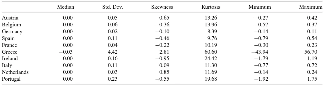
Table 1 provides summary statistics for daily demeaned changes in these 10 CDS spreads. All time series have significant non-Gaussian features under standard tests and significance lev-els. In particular, we note the nonzero skewness and large values of kurtosis for almost all time series in the sample. All series are covariance stationary according to standard unit root (ADF) tests.
3.2 Daily Model Calibration
We estimate all model parameters over the entire sample. Us-ing the parameter estimates, we compute joint and conditional default probabilities after calibrate the model at each timetto market implied individual probabilities of default as in Sego-viano and Goodhart (2009).
The marginal default probabilities are typically estimated directly from observed prices of CDS insurance. We invert a CDS pricing formula to calculate the risk neutral default prob-abilities following the procedure described in O’Kane (2008). This “bootstrapping” procedure is a standard method in finan-cial practice for marking to market a CDS contract. Since the
Table 1. CDS descriptive statistics
Median Std. Dev. Skewness Kurtosis Minimum Maximum
Austria 0.00 0.05 0.65 13.26 −0.27 0.42
Belgium 0.00 0.06 −0.36 13.96 −0.57 0.37
Germany 0.00 0.02 −0.10 8.39 −0.14 0.11
Spain 0.00 0.11 −0.46 9.76 −0.79 0.54
France 0.00 0.04 −0.22 10.19 −0.30 0.23
Greece −0.03 4.42 2.81 60.60 −43.94 56.70
Ireland 0.00 0.16 −0.95 24.42 −1.79 1.19
Italy 0.00 0.11 0.09 11.30 −0.77 0.72
Netherlands 0.00 0.03 0.85 11.69 −0.14 0.24
Portugal 0.00 0.23 −0.55 19.68 −1.92 1.75
Note: The summary statistics correspond to daily changes in observed sovereign CDS spreads (in 100 basis points) for 10 euro-area countries from January 2008 to February 2013. Almost all skewness and excess kurtosis statistics havep-values below 10−4, except the skewness parameters of Germany and Italy.
procedure is standard and available in O’Kane (2008), we only highlight our choices in the implementation. First, we fix the recovery rate at a stressed level of 25% for all countries. This is roughly in line with the recovery rate that investors received on average in the Greek debt restructuring in Spring 2012, see Zettelmeyer, Trebesch, and Gulati (2013). Second, the term structure of discount ratesrt is flat at the one year EURIBOR
rate (and thus close to zero in our later application). Also, the risk neutral default intensity is assumed to be constant. We note, however, that the precise form of discounting hardly has an effect on our results as the implied risk neutral default intensi-ties are quite robust to the precise form of discounting. Finally, we use a CDS pricing formula that does not take into account counterparty credit risk; see also Huang, Zhou, and Zhu (2009), Black et al. (2012), and Creal, Gramacy, and Tsay (2012). Given these choices, a solver quickly finds the (unique) default inten-sity that matches the expected present values of payments within the premium leg and within the default leg of the CDS. The one year ahead default probability is a simple function of the default intensity; see O’Kane (2008) and Hull and White (2000).
Given the marginal probability of defaultpi,t of sovereigni
at timet, we simulate the joint probability of defaultpij,t for
sovereignsiandjat timetas
pij,t =Pryi,t> Fi,t−1(pi,t), yj,t > Fj,t−1(pj,t), (9)
whereyi,t is theith element of yt, andFi,t−1(·) denotes the
in-verse marginal GHST distribution of sovereigniat timet, and where the joint probability of exceedance is computed using the multivariate GHST dependence structure. All marginal and joint GHST probabilities are computed using the model’s esti-mated parameters. The conditional probability for sovereignj
defaulting given a default of sovereigniis easily computed as
pij,t/pi,t. Note that the joint and conditional default
probabili-ties have a dual time dependence. First, there is dependence on time because the model is recalibrated to current market condi-tionspi,t at each timet. Second, there is dependence on time
because volatilities and correlations vary over time. The second effect impacts both the marginal distributions of yi,t and the
joint distribution ofytas specified in Section2.
3.3 Time-Varying Volatility and Correlation
This section discusses our main empirical results on time-varying volatility and correlation dynamics based on the GHST
modeling framework in Section 2. We consider four
differ-ent choices for the time-varying parameter model specifica-tion. The first three correspond to a Gaussian (ν= ∞,γ =0), a Student’s-t (γ =0), and a GHST multivariate distribution, respectively. The fourth approach uses GHST univariate dis-tributions for the marginal disdis-tributions, and a GHST copula for the dependence structure. The copula approach is flexible in allowing for heterogeneity across sovereigns in the marginal behavior of CDS spread changes. The computational burden for the dependence part, however, is challenging. This is due to the required numerical inversion of the cumulative distribution function of the GHST for every observation at every evaluation of the likelihood. To facilitate this task, we restrict the number of parameters in the copula by settingγ =γ˜(1, . . . ,1)′for some
scalar ˜γ ∈R. Note that we still allow for different skewness parameters for each of the marginal distributions. Also note that the degrees of freedom parameter may be different for each of the marginal distributions, as well as for the marginal distribu-tions and the copula.
In an earlier version of this article we also considered a GHST model for a fixed degrees of freedom parameterν=5. The pa-rameterνis then treated as a robustness parameter as in Franses and Lucas (1998). The main advantage of fixingνis that it in-creases the computational speed considerably, while most of the qualitative results in terms of the dynamics of joint and condi-tional default probabilities remain unaltered for the application
at hand. We leave the suggestion of using a predetermined ν
as a robustness device for empirical researchers who are more concerned about computational speed.
There is one important difference between the multivariate GHST and the copula GHST approach that is relevant for the results reported below. The multivariate GHST restricts the degrees of freedom parameter to be the same across all the marginals. As a result, the degrees of freedom parameter determines both the fatness of the marginal tails and the degree of tail clustering. Some of the CDS data have very fat tails,
pushing the value ofν downwards. However, asν approaches
4 from above, the covariance matrixtcollapses to a rank one
matrix proportional to γ γ′, and thus to a perfect correlation
2008 2009 2010 2011 2012 2013 0.005
0.010 0.015 0.020
Germany, squared difference CDS
2008 2009 2010 2011 2012 2013 1
2 3 4
Portugal, squared difference CDS
2008 2009 2010 2011 2012 2013 0.005
0.010
Germany, Gaussian volatility Germany, Student-t scale
Germany, GHST scale Germany, GHST marginal scale
2008 2009 2010 2011 2012 2013 0.5
1.0 1.5 2.0
Portugal, Gaussian volatility Portugal, Student-t scale
Portugal, GHST scale Portugal, GHST marginal scale
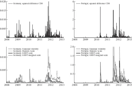
Figure 1. Estimated time-varying volatilities for changes in CDS for two countries. We report four different estimates of time-varying volatility that pertain to changes in CDS spreads on sovereign debt. The estimates are based on different parametric assumptions regarding the univariate distribution of sovereign CDS spread changes: Gaussian, symmetrict, and a GHST distribution, and a GHST copula. We pick two countries, Germany and Portugal, to illustrate differences across model specifications. As a direct benchmark, squared CDS spread changes are plotted as well in the top panels.
case. As this is incompatible with the data, there is an automatic mechanism to pushν above 4. The final result balances these two effects. In the copula approach, the step of modeling the marginals versus the dependence structure is split. As a result, the degrees of freedom parameter for the marginal models may become very low, while that for the copula can be substantially higher; see also the empirical results further below. In particular, the degrees of freedom parameters of the marginal models may be below 4, such that the variance no longer exists. This poses no problem for the computation of joint and conditional de-fault probabilities. It does mean, however, that we can no longer consider a time-varyingvariancefor the marginals. To account for this, we setT =1 for the marginal models in the copula
approach and interpretLt as the time-varyingscaleparameter.
The latter is well-defined for anyν >0.
Figure 1plots the squared CDS spread changes and estimated volatility or scale levels for two countries and four different mod-els. The assumed statistical model (Gaussian, Student-t, GHST, copula) directly influences the dynamics of the volatility esti-mates. For example, early 2010, the German series spikes for the Gaussian model and then comes down exponentially. For Portugal we see something similar around July 2011. In partic-ular, the temporary increased volatility for the Gaussian series does not appear in line with the subsequent squared CDS spread changes. We see no similar behavior for the GAS models based on fat-tailed distributional assumptions due to the presence of the weighting mechanismwtin (7).
Table 2reports the parameter estimates of the different mod-els. We estimate all specifications under the restriction of sta-tionarity by reparameterizingB=(1+exp(−B˜))−1for ˜B
∈R. Standard errors are computed using the likelihood based sand-wich covariance matrix estimator and the delta method. For all models, volatilities and correlations are highly persistent, that is,Bis numerically equal to or close to one. Note that the pa-rameterization of our score driven model is different than that of a standard GARCH model. In particular, the persistence is
com-pletely captured byBrather than byA+B as in the GARCH
case. Also note thatωregularly takes on negative values. This is natural as we defineftto be the log-volatility rather than the
volatility itself.
The estimates of the skewness parametersγ differ somewhat between the multivariate GHST and the GHST copula speci-fication. For the multivariate GHST, 7 out of the 10 γ’s are negative, but only those for Greece, Ireland, and Portugal are statistically significant. For the copula, all marginalγ’s are pos-itive, but the (common) copulaγ is negative. The significance of the marginalγ’s differs between countries. The copula γ, however, is highly significant. The difference can be explained by the fact that the multivariate distribution mixes the effect of the marginal distributions with that of the dependence structure. This is no longer the case for the copula. The negativeγ for the copula increases the sensitivity of the correlation dynamics to common increases in CDS spreads, making sudden com-mon shifts upwards in CDS spreads more likely. The (marginal)
Table 2. Model parameter estimates
AT BE DE ES FR GR IE IT NL PT Joint
Gaussian
A 0.058 0.070 0.075 0.066 0.085 0.096 0.073 0.092 0.082 0.089 0.015 (0.007) (0.020) (0.013) (0.036) (0.011) (0.005) (0.017) (0.012) (0.016) (0.008) (0.001) B 0.992 0.993 0.978 0.983 0.993 1.000 0.969 1.000 0.982 1.000 0.983
(0.003) (0.010) (0.011) (0.022) (0.007) (0.000) (0.010) (0.000) (0.010) (0.000) (0.002) ω −3.551 −3.684 −4.065 −2.546 −3.952 −3.648 −2.326 −4.211 −3.954 −3.934
(0.314) (0.803) (0.150) (0.289) (0.412) (0.294) (0.147) (0.261) (0.196) (0.319) Student’s-t
A 0.127 0.126 0.110 0.136 0.138 0.148 0.150 0.138 0.125 0.184 0.022 (0.011) (0.010) (0.014) (0.014) (0.017) (0.034) (0.020) (0.014) (0.015) (0.025) (0.002) B 1.000 1.000 1.000 1.000 1.000 0.999 1.000 1.000 1.000 0.999 1.000
(0.000) (0.000) (0.000) (0.001) (0.000) (0.001) (0.000) (0.000) (0.000) (0.001) (0.000) ω −3.955 −3.405 −3.983 −3.540 −3.504 −3.616 −3.476 −3.436 −3.912 −3.502
(0.337) (0.242) (0.281) (0.280) (0.342) (0.279) (0.506) (0.284) (0.296) (0.318)
ν 5.917
(0.210) GHST
A 0.081 0.079 0.071 0.087 0.089 0.094 0.096 0.088 0.080 0.117 0.013 (0.008) (0.007) (0.011) (0.010) (0.011) (0.025) (0.013) (0.009) (0.011) (0.016) (0.001) B 0.998 0.998 0.999 0.997 0.998 0.995 0.996 0.997 0.998 0.995 1.000
(0.001) (0.001) (0.001) (0.001) (0.001) (0.002) (0.001) (0.001) (0.001) (0.001) (0.000) ω −3.787 −3.163 −3.765 −3.343 −3.312 −2.863 −3.288 −3.284 −3.703 −3.342
(0.350) (0.255) (0.293) (0.293) (0.349) (0.301) (0.472) (0.290) (0.327) (0.329)
ν 4.048
(0.021) γ −0.009 −0.004 0.005 −0.023 −0.002 0.165 −0.024 0.000 −0.008 −0.039
(0.021) (0.017) (0.013) (0.020) (0.014) (0.036) (0.012) (0.013) (0.011) (0.016) GHST Copula
A 0.098 0.099 0.119 0.120 0.135 0.197 0.128 0.105 0.103 0.125 0.007 (0.012) (0.014) (0.017) (0.016) (0.017) (0.028) (0.016) (0.015) (0.016) (0.014) (0.001) B 0.993 0.991 0.974 0.989 0.985 0.985 0.990 0.991 0.983 0.991 0.993
(0.004) (0.004) (0.009) (0.004) (0.006) (0.004) (0.004) (0.004) (0.007) (0.003) (0.001) ω −3.530 −3.422 −4.305 −2.689 −3.843 −1.330 −2.572 −2.736 −4.172 −2.219
(0.457) (0.347) (0.159) (0.345) (0.294) (0.362) (0.402) (0.385) (0.199) (0.439)
ν 3.742 4.115 4.452 3.989 4.316 2.074 3.028 3.894 3.638 4.590 10.291 (0.419) (0.487) (0.567) (0.436) (0.552) (0.070) (0.279) (0.460) (0.454) (0.619) (1.049) γ 0.077 0.090 0.056 0.056 0.085 0.013 0.020 0.070 0.059 0.119 −0.008
(0.029) (0.035) (0.034) (0.028) (0.035) (0.012) (0.016) (0.030) (0.029) (0.041) (0.001)
Note: The table reports parameter estimates that pertain to four different model specifications. The sample consists of daily changes from January 2008 to February 2013. The Student’s-t
and GHST distribution are estimated jointly. The GHST copula is estimated with the same skewness parameter.
volatility dynamics, by contrast, appear less sensitive to large increases in CDS spreads, as follows from the positiveγ’s for the marginal models. The multivariate GHST specification lacks this flexibility.
The degrees of freedom parameter for the Student’s-t distri-bution is estimated atν=5.9. That of the multivariate GHST distribution is estimated even lower atν=4.05. This is close to the region where the variance no longer exists. As discussed
before, the low value ofν for the GHST mixes the extremely
fat-tailed marginal behavior of CDS spread changes for spe-cific countries such as Greece or Ireland, and the multivariate tail dependence structure. The GHST copula approach does not suffer from this automatic link. For the copula specification, we indeed see that six countries have a degrees of freedom estimate for the marginal distribution below 4. For the Greek case, the estimate is even close to 2, such that the mean may
no longer exist. By contrast, the degrees of freedom parame-ter for the dependence structure is estimated atν=10.3, such that tail dependence for the copula specification is smaller. How the different effects balance out when computing the joint and conditional default probabilities is shown in the next sections.
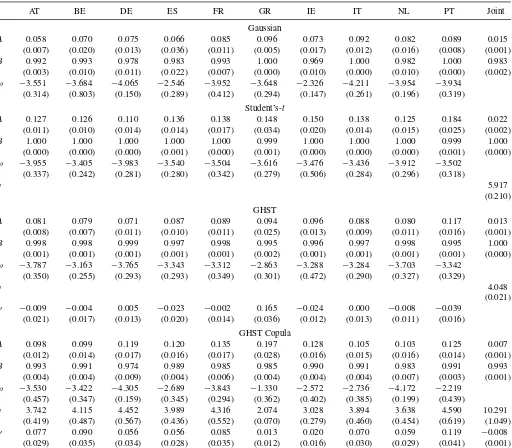
Figure 2 plots the average correlation, averaged across 45 bivariate time-varying pairs, for each model specification. The dynamic correlation coefficients refer to the standardized CDS spread changes. Givenn=10, there aren(n−1)/2=45 dif-ferent elements in the correlation matrix. As a robustness check, we benchmark each multivariate model-based estimate to the av-erage over 45 correlation pairs obtained from a 60 business days rolling window. Over each window we use the same prefiltered marginal data as for the multivariate model estimates. Com-paring the correlation estimates across different specifications,
2008 2009 2010 2011 2012 2013 0.25
0.50 0.75 1.00
Gaussian Correlation Rolling Window Correlation
2008 2009 2010 2011 2012 2013 0.25
0.50 0.75 1.00
Student-t correlation Rolling Window Correlation
2008 2009 2010 2011 2012 2013 0.25
0.50 0.75 1.00
GHST correlation Rolling Window Correlation
2008 2009 2010 2011 2012 2013 0.25
0.50 0.75 1.00
GHST copula correlation Rolling Window Correlation
Figure 2. Average correlation over time. Plots of the estimated average correlation over time, where averaging takes place over 45 estimated correlation coefficients. The correlations are estimated based on different parametric assumptions: Gaussian, symmetrict, and GH Skewed-t (GHST), and GHST copula. The time axis runs from March 2008 to February 2013. The corresponding rolling window correlations are each estimated using a window of 60 business days of prefiltered CDS changes.
the GHST model matches the rolling window estimates most closely.
Correlations increased visibly during times of stress. GHST correlations are low in the beginning of the sample at around 0.3 and increase to around 0.75 during 2010 and 2011. Estimated dependence across euro area sovereign risk increases sharply for the first time around September 15, 2008, on the day of the Lehman bankruptcy, and around September 30, 2008, when the Irish government issued a broad guarantee for the deposits and borrowings of six large financial institutions. Average GHST correlations remain high afterwards, around 0.75, until around May 10, 2010. At this time, euro area heads of state introduced a rescue package that contained government bond purchases by the ECB under the so-called Securities Markets Program, and the European Financial Stability Facility, a fund designed to provide financial assistance to euro area states in economic difficulties. After an eventual decline to around 0.5 toward the beginning of 2013.
3.4 Joint Sovereign Risk During the Euro
Area Debt Crisis
This section discusses the probability of the extreme (tail) possibility that two or more credit events take place in our sample of 10 euro-area countries, over a one year horizon, as perceived by credit market participants. Such a probability depends on the perceived country-specific (marginal) probabilities, as well as the dependence structure.
Figure 3 plots estimates of marginal CDS-implied prob-abilities of default (pd) over a one year horizon obtained as
described in Section 3.2and in, for example, Segoviano and
Goodhart (2009). These probabilities are directly inferred from CDS spreads and do not depend on parametric assumptions regarding their joint distribution. Market-implied pds vary markedly in the cross-section, ranging from below 2% for some countries to above 8% for Greece, Portugal, and Ireland during the second half of 2011. The market-implied probability of a credit event in Greece increases above 25% in mid-2011, and afterwards increases further until March 2012.
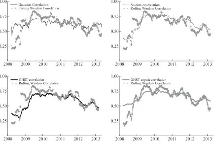
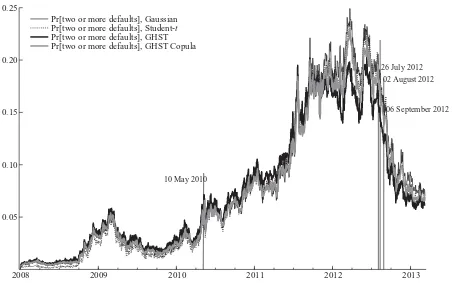
Figure 4plots the market-implied probability of two or more credit events among 10 euro-area countries over a one year horizon. The joint probability is calculated by simulation, using 50,000 draws at each timet. For each simulation, we keep track of the joint exceedance ofyi,t andyj,t above their calibrated
thresholds at timet, as described in Section 3.2. This simple estimate combines all marginal risk estimates and 45 correla-tion parameter estimates into a single time series plot. The plot reflects, first, the deterioration of debt conditions since the be-ginning of the debt crisis in Spring 2010, and second, a clear turning of the tide around mid-2012. Vertical lines indicate the announcement of a first euro area rescue package (the EFSF and SMP) on May 10, 2010, and announcements regarding the Out-right Monetary Transactions (OMT) in August and September 2012, which we revisit in Section4.
There are only slightly different patterns in the estimated probabilities of joint default inFigure 4; the overall dynamics are
Austria, AT Belgium, BE Germany, DE Spain, ES France, FR Greece, GR Ireland, IE Italy, IT
The Netherlands, NL Portugal, PT
2008 2009 2010 2011 2012 2013
0.05 0.10 0.15 0.20 0.25
GR
PT
IE
ES
IT
BE FR
AT NL DE
Austria, AT Belgium, BE Germany, DE Spain, ES France, FR Greece, GR Ireland, IE Italy, IT
The Netherlands, NL Portugal, PT
Figure 3. CDS-implied marginal probabilities of a credit event. The risk neutral marginal probabilities of a credit event for 10 euro area countries are extracted from CDS prices. The sample is daily data from January 1, 2008 to February 28, 2013.
2008 2009 2010 2011 2012 2013
0.05 0.10 0.15 0.20 0.25
10 May 2010
02 August 2012
06 September 2012 26 July 2012
Pr[two or more defaults], Gaussian Pr[two or more defaults], Student-t
Pr[two or more defaults], GHST Pr[two or more defaults], GHST Copula
Figure 4. Probability of two or more credit events. The top panel plots the time-varying probability of two or more credit events (out of 10) over a one-year horizon. Estimates are based on different distributional assumptions regarding marginal risks and multivariate de-pendence: Gaussian, symmetric-t, and GH skewed-t(GHST) distribution, and a GHST copula with GHST marginals. Vertical lines refer to program announcements on May 10, 2010 (SMP and EFSF), and on August 2, 2012 (OMT) and September 6, 2012 (details on OMT); see Section4.
roughly similar across the different distributional specifications. In the beginning of our sample, the joint default probability from the GHST multivariate distribution is somewhat higher
than that from the Gaussian, symmetric-t, and GHST copula
models. This pattern reverses in mid-2011, when the Gaussian, symmetric-t, and GHST copula estimates are slightly higher than the GHST multivariate density estimate. Altogether, the level and dynamics in the estimated measures of joint default from this section do not appear to be very sensitive to the precise model specification.
3.5 Conditional Risk and Risk Spillovers
This section investigates conditional probabilities of default. Such conditional probabilities relate to questions of “what if?” In addition, a cross-sectional comparison may help reveal which entities are expected by credit markets to be relatively more af-fected by a certain credit event. To our knowledge, this is the first attempt in the literature to evaluate such market perceptions. Clearly, conditioning on a credit event is different from condi-tioning on incremental changes in risk; see Caceres, Guzzo, and Segoviano (2010) and Caporin et al. (2012b).
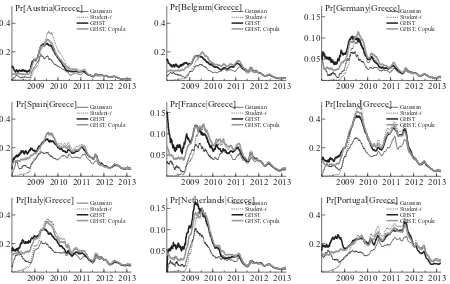
We condition on a credit event in Greece to illustrate our general methodology. We pick this event since it has by far the highest market-implied probability of occurring during most of our sample period, and indeed occurred on March 8, 2012.
Figure 5plots the conditional probability of a credit event, as perceived by credit markets, for nine euro-area countries. We again consider the four parametric multivariate models consid-ered in the previous sections.
We document three empirical findings. First, during 2011 Ireland and Portugal are perceived by credit market participants to be more affected by a possible Greek credit event than the other countries, with conditional probabilities around 30%; this is similar for all fat-tailed parametric specifications. The condi-tional probability estimates for the Gaussian model are lower at a level slightly above 20%. Ireland and Portugal were in an EU-IMF program during 2011. The other seven countries appear more “ring-fenced” during that time, with conditional probabil-ities below 20%. As a result, credit market participants appear to be most concerned about the adverse fallout for countries that are already in a fiscally weaker position. This is intuitive, for example, because sovereign fiscal backstops for the financial sector are less strong.
Second, the level and dynamics of the conditional estimates are clearly sensitive to the parametric assumptions. The con-ditional probability estimates are highest in the GHST density and copula case, with the symmetric-testimates second, and the Gaussian case last. The correlations and the mixing variableςt
in Equation (1) thus operate together to capture the tail depen-dence in the data. Accounting for this tail dependepen-dence changes the conditional risk assessments.
Finally, and interestingly, the conditional probabilities decrease markedly since the second half of 2011. This is a time when the CDS-implied marginal probability of a Greek credit event increases from about 25% to close to one (>90% in December 2011). As the eventual default becomes more and more likely, and is eventually almost entirely priced into CDS contracts and sovereign bonds, also the perceived fallout for the other countries in our sample is reduced. This is consistent with
2009 2010 2011 2012 2013 0.2
2009 2010 2011 2012 2013 0.2
2009 2010 2011 2012 2013 0.05
2009 2010 2011 2012 2013 0.2
2009 2010 2011 2012 2013 0.05
0.10
0.15 Pr[France|Greece] Gaussian Student-t
GHST GHST, Copula
2009 2010 2011 2012 2013 0.2
2009 2010 2011 2012 2013 0.2
2009 2010 2011 2012 2013 0.05
0.10
0.15 Pr[Netherlands|Greece]Gaussian Student-t
GHST GHST, Copula
2009 2010 2011 2012 2013 0.2
Figure 5. Conditional probabilities of a credit event given a Greek credit event. Plots of annual conditional probabilities of a credit event for nine countries in the euro area given a credit event in Greece. We distinguish conditional risk estimates based on a Gaussian dependence structure, symmetric-t, GH skewed-t(GHST) multivariate density, and a GHST copula with GHST marginals.
the notion that market participants prepare for the contingency of a credit event as it becomes more and more apparent. When the credit event actually happened, it was widely anticipated and markets were relatively unfazed; see Reuters(2012).
4 EVENT STUDY: ASSET PURCHASE
ANNOUNCEMENTS AND SOVEREIGN RISK DEPENDENCE
This section investigates the immediate impact of two key policy announcements on sovereign risk conditions as perceived by credit market participants. We document that each policy announcement had a very strong effect on joint sovereign risk perceptions, cutting some perceived joint risks by up to 50%. We show that this pronounced impact worked through decreasing marginal risks, and not by lowering risk dependence. For all analyses in this section, we use the GHST copula specification of the model as it is the most flexible specification.
During a weekend meeting on May 8–9, 2010, euro area heads of state agreed on a comprehensive rescue package to mitigate potential risk contagion in the euro area. Two main measures were announced on the same day: the European Finan-cial Stability Facility (EFSF) and the ECB’s Securities Markets Program (SMP). The EFSF is a limited liability facility with an objective to preserve financial stability of the euro area by providing temporary financial assistance to euro area member states in economic difficulties. Initially committed funds were 440bn Euro. The announcement made clear that EFSF funds could be combined with funds raised by the European Com-mission of up to 60bn Euro, and funds from the International Monetary Fund of up to 250bn Euro, for a total safety net up to 750bn Euro. The other key component of the rescue package was a government bond buying program, the SMP. Specifically, the ECB announced that it would start to intervene in secondary government bond markets to ensure depth and liquidity in those market segments that are qualified as being dysfunctional. These purchases were meant to restore an appropriate monetary policy transmission mechanism; see ECB (2010). The joint announce-ment impacted asset prices on Monday, May 10, 2010.
The impact of the May 10, 2010 announcement on joint sovereign risk perceptions (as well as that of the initial bond purchases) is visible inFigure 4. The figure suggests that the probability of two or more credit events in our sample of 10 countries decreases from about 7% to approximately 3% before and after the announcement, thus virtually overnight.Figure 3
indicates that marginal risks decreased considerably as well. The average correlation plots inFigure 2do not suggest a widespread and prolonged decrease in dependence. Instead, there seems to be an up-tick in average correlations.
To further investigate the impact on joint and conditional sovereign risk from actions communicated on May 10, 2010
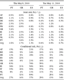
and implemented shortly afterwards, Table 3 reports
model-based estimates of joint and conditional risk. We report our risk estimates for two dates, Thursday, May 6, 2010 and Tuesday, May 11, 2011, that is, two business days before and after the announced change in policy. The top panel ofTable 3confirms that the joint probability of a credit event in, say, both Portugal and Greece, or Ireland and Greece, declines from 3.8% to 1.7% and from 2.5% to 1.3%, respectively. These are large declines in
Table 3. Sovereign risk perceptions around SMP and EFSF announcement Conditional risk, Pr(i|j)
AT 15% 8% 21% 17% 8% 20%
Note: The top and bottom panels report GHST copula model-implied joint and conditional probabilities of a credit event for a subset of countries, respectively. For the conditional probabilities Pr(idefaulting|jdefaulted), the conditioning eventsjare in the columns (PT, GR, ES), while the eventsiare in the rows (AT, BE,. . ., PT). Avg contains the averages for each column. Joint and conditional risks are reported two business days before and after the 10 May 2010 announcement.
joint risk, cutting some perceived risks in half. For any country in the sample, the probability of that country failing simultaneously with Greece or Portugal over a one-year horizon is substantially lower after the May 10, 2010 announcement than before. The bottom panel of Table 3 indicates that the decrease in joint default probabilities is generally not due to a decline in default dependence. Instead, the perceived conditional probabilities of a credit event in, for example, Greece or Ireland given a credit event in Portugal remains roughly constant from 63% to 59% and from 38% to 38%, respectively. Similarly, the perceived conditional probabilities of a credit event in Belgium or Ireland given a credit event in Greece only move from 9% to 11% and from 21% to 19%, respectively.
Figures 4 and 3 also suggest that the impact of the May
10, 2010 announcement was temporary. Sovereign yields soon started to rise afterwards in some euro-area countries.Figure 4
would suggest that the height of the euro area debt crisis could be dated from mid-2011 to mid-2012.
A visible break of the upward trend in joint risk can be asso-ciated with three dates in 2012 (also visible as vertical lines in
Figure 4). On July 26, 2012, the president of the ECB pledged to do “whatever it takes” to preserve the euro, and that “it will be enough.” In the speech, sovereign risk premia were mentioned as a key concern within the ECB’s mandate; see Draghi (2012). Communication regarding a new asset purchase program, the
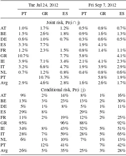
Table 4. Sovereign risk perceptions around OMT announcements Conditional risk, Pr(i|j)
AT 9% 2% 14% 8% 1% 16%
Note: The top and bottom panels report GHST copula model-implied joint and conditional probabilities of a credit event for a subset of countries, respectively. For the conditional probabilities Pr(idefaulting|jdefaulted), the conditioning eventsjare in the columns (PT, GR, ES), while the eventsiare in the rows (AT, BE,. . ., PT). Avg contains the averages for each column. Joint and conditional risks are reported two business days before the July 26, 2012, and after the 06 September 2012 announcement of the OMT details.
Outright Monetary Transactions (OMT), followed swiftly af-terwards on August 2. The OMT is an asset purchase program that replaces the earlier SMP; see ECB (2012) for details. These details on OMT were communicated on September 6, 2012. The joint impact of the three measures on joint risk in clearly visible in Figure 4. For a discussion of this figure in the context of central bank communication in the financial press, see Wessel (2013).
Table 4reports model-based estimates of joint and conditional risk around the OMT announcements. We compare risk esti-mates for Tuesday, July 24, 2012 (two days before the speech) to risk estimates for Friday, September 7, 2012 (two days af-ter the announcement of the OMT details). A common finding emerges. Just as in the case of the May 10, 2010 announcement, joint risks have decreased markedly. For example, the joint prob-ability of a credit event in both Spain and Italy over a one year horizon decreased from 4.7% to 2.9%. Similar reductions are observed for other countries as well. Second, the decrease in joint risk is generally not due to a decline in dependence, or per-ceived connectedness. Instead, the conditional probabilities of a credit event remain very similar, despite the period of more than two months between the two measurement dates. This suggests that market perceptions regarding risk interactions remained a concern.
We conclude that both the May 10, 2010 and 2012 policy announcements had a very strong effect on joint sovereign risk
perceptions, cutting some perceived joint risks by up to 50%. This pronounced impact worked through decreasing marginal risks, not perceived risk dependence. These findings are robust to alternative statistical choices (such as the degrees of freedom in the dependence model), as well as to alternative ways of extracting marginal risks from CDS prices (such as recovery rates assumptions in the case of a credit event).
5 CONCLUSION
We have proposed a novel empirical framework to assess risk perceptions regarding joint and conditional default based on the price of CDS insurance. Our methodology is novel in that our joint risk measures are derived from a multivariate framework based on a dynamic generalized hyperbolic skewed-tconditional density that naturally accommodates skewed and heavy-tailed changes in marginal risks as well as time variation in volatility and multivariate dependence. When applying the model to euro area sovereign CDS data from January 2008 to February 2013, we find significant time variation in risk dependence, evidence for risk spillovers regarding sovereign credit events, as well as a strong impact of key policy announcements during the euro area debt crisis on joint and conditional sovereign risk perceptions. Regarding model risk, parametric assumptions, in particular assumptions about higher order moments and their dynamics, matter for joint and conditional risk assessments.
APPENDIX A: TECHNICAL BACKGROUND
The generalized autoregressive score model of Creal,
Koop-man, and Lucas (2001, 2013) for the GH skewed-t (GHST)
conditional density (2) adjusts the time-varying parameterft at
every step using the scaled score of the conditional density at timet. This can be regarded as a steepest ascent improvement of the parameter using the local (at timet) likelihood fit of the model. ftD =ln(diag(Dt)), which ensures that variances are always
positive, irrespective of the value of ftD. For the correlation matrix, we use the hypersphere parameterization also used in Creal, Koopman, and Lucas (2011) and Zhang et al. (2011). This ensures thatRt is always a correlation matrix, that is, positive
semidefinite with ones on the diagonal. We setRt =R(ftR)=
wherecij t =cos(φij t) andsij t =sin(φij t). The dimension offtR
thus equals the number of correlation pairs.
As implied by Equation (6), we take the derivative of the log conditional density with respect toft, and obtain
∇t =
modified Bessel function of the second kind, D0
n is the the
duplication matrix vec(L)=D0
nvech(L) for a lower triangular
matrixL,Dnis the standard duplication matrix for a
symmet-ric matrixS vec(S)=Dnvech(S),Bn=(D′
nDn)−1Dn′, andCn
is the commutation matrix, vec(S′)=Cnvec(S) for an arbitrary
matrixS.
To scale the score∇t, Creal, Koopman, and Lucas (2013)
pro-posed the use of powers of the inverse information matrix. The information matrix for the GHST distribution, however, does not have a tractable form. Therefore, we scale by the information matrix of the symmetric Student’s-tdistribution,
St = {′
t(I⊗(LtT)−1)′[gG−vec(I)vec(I)′]
×(I⊗(LtT)−1)t}−1, (A.8)
where g=(ν+n)/(ν+2+n), and G=E[ztz′t⊗ztz′t] for zt ∼N(0,I). Zhang et al. (2011) demonstrated that this results
in a stable model that outperforms alternatives such as the DCC if the data are fat-tailed and skewed.
For parsimony, the dynamics of the correlation parameterfR t
follow a similar parameterization as in the DCC model,
ftR+1=ω˜(1−BR) ¯fR+ARstR+BRftR, (A.9)
where ˜ω, AR, BR ∈Rare scalars, and ¯fR is such that R( ¯fR)
equals the unconditional correlation matrix of the data. Estima-tion results showed that ˜ωwas close to 1 in all cases. To further reduce the number of parameters, we therefore set ˜ω=1. All remaining parameters are estimated by maximum likelihood. Inference is carried out by taking the negative inverse Hessian of the log-likelihood at the optimum as the covariance matrix for the estimator.
Evaluating the GHST density and distribution can be tricky due to the modified Bessel function and various off-setting
fac-tors in the conditional density expression (2). We used the built-in modified Bessel function of the Ox programmbuilt-ing language of Doornik (2007), except in the far tails. For the far tails and
yt, γ ∈R, we used the expression
Abramowitz and Stegun (1970). This also directly balances the skewness effect in either tail in a numerically stable way. If small values of the argument|b|are of interest, similar expan-sions exist.
ACKNOWLEDGMENTS
The authors thank seminar and conference participants at Bundesbank, HEC Lausanne, Riksbank, the Royal Economics Society meeting at Cambridge, the IRMC risk management conference in Rome, the Society for Financial Econometrics meeting in Oxford, the Econometric Society European Meet-ing in Malaga, the “ForecastMeet-ing rare events” conference at San Francisco Fed, the Macro-prudential Research Network annual conference at ECB, the “New tools for financial regulation” con-ference at Banque de France, and the Humboldt-Copenhagen Conference in Financial Econometrics in Berlin. Andr´e Lucas thanks the Dutch National Science Foundation (NWO, grant VICI453-09-005) and the European Union Seventh Framework Programme (FP7SSH/20072013, grant agreement 320270 -SYRTO) for financial support. The views expressed in this arti-cle are those of the authors and they do not necessarily reflect the views or policies of the Riksbank, the European Central Bank, or the European System of Central Banks.
[Received June 2012. Revised May 2013.]
REFERENCES
Aas, K., and Haff, I. (2006), “The Generalized Hyperbolic Skew Student’st Distribution,”Journal of Financial Econometrics, 4, 275–309. [273] Abramowitz, M., and Stegun, I. A. (1970),Handbook of Mathematical Function
with Formulas, Graphs, and Mathematical Tables, (Applied Mathematics Series, Vol. 55), National Bureau of Standards, U.S. Department of Com-merce. [283]
Acharya, V. V., Pedersen, L. H., Philippon, T., and Richardson, M. (2010), “Measuring Systemic Risk,” FRB of Cleveland Working Paper No. 10-02. [272]
Ang, A., and Longstaff, F. (2011), “Systemic Sovereign Credit Risk: Lessons From the US and Europe,” NBER Discussion Paper 16983. [272,274] Avesani, R. G., Pascual, A. G., and Li, J. (2006), “A New Risk Indicator and
Stress Testing Tool: A Multifactor Nth-to-Default cds Basket,” Working Paper, WP/06/105, IMF. [272]
Azzalini, A., and Capitanio, A. (2003), “Distributions Generated by Perturbation of Symmetry With Emphasis on a Multivariate SkewtDistribution,”Journal of the Royal Statistical Society, Series B, 65, 367–389. [273]
Bauwens, L., and Laurent, S. (2005), “A New Class of Multivariate Skew Den-sities, With Application to Generalized Autoregressive Conditional Het-eroskedasticity Models,”Journal of Business and Economic Statistics, 23, 346–354. [273]
Benzoni, L., Collin-Dufresne, P., Goldstein, R., and Helwege, J. (2011), “Mod-eling Credit Contagion via the Updating of Fragile Beliefs,” available at http://papers.ssrn.com/sol3/papers.cfm?abstract_id=2016579. [272] Black, L., Correa, R., Huang, X., and Zhou, H. (2012), “The Systemic Risk of
European Banks During the Financial and Sovereign Debt Crisis,” avail-able at http://www.federalreserve.gov/pubs/ifdp/2013/1083/ifdp1083.pdf. [271,275]
Boudt, K., Danielsson, J., and Laurent, S. (2013), “Robust Forecasting of Dy-namic Conditional Correlation GARCH Models,”International Journal of Forecasting, 29, 244–257. [274]
Branco, M., and Dey, D. (2001), “A General Class of Multivariate Skew-Elliptical Distributions,”Journal of Multivariate Analysis, 79, 99– 113. [273]
Caceres, C., Guzzo, V., and Segoviano, M. (2010), “Sovereign Spreads: Global Risk Aversion, Contagion or Fundamentals?” Working Paper WP/10/120, IMF. [280]
Caporin, M., Pelizzon, L., Ravazzolo, F., and Rigobon, R. (2012a), “Measur-ing Sovereign Contagion in Europe,” available athttp://ideas.repec.org/ p/bno/worpap/2012_05.html. [272]
——— (2012b), “Measuring Sovereign Contagion in Europe,” available at http://www.nber.org/papers/w18741.. [280]
Chen, Y., H¨ardle, W., and Spokoiny, V. (2010), “GHICA—Risk Analysis With GH Distributions and Independent Components,”Journal of Empirical Fi-nance, 17, 255–269. [272]
Christoffersen, P., Errunza, V., Jacobs, K., and Langlois, H. (2012), “Is the Potential for International Diversification Disappearing? A Dy-namic Copula Approach,” Review of Financial Studies, 25, 3711– 3751. [272]
Creal, D., Koopman, S. J., and Lucas, A. (2011), “A Dynamic Multivariate Heavy-Tailed Model for Time-Varying Volatilities and Correlations,” Jour-nal of Economic and Business Statistics, 29, 552–563. [272,273,282] ——— (2013), “Generalized Autoregressive Score Models With Applications,”
Journal of Applied Econometrics, 28(5), 777–795. [272,273,282,283] Creal, D. D., Gramacy, R. B., and Tsay, R. S. (2012), “Market-Based
Credit Ratings,” available at http://faculty.chicagobooth.edu/drew.creal/ research/papers/crealGramacyTsay2012.pdf. [275]
DeGrauwe, P., and Ji, Y. (2012), “Mispricing of Sovereign Risk and Multiple Equilibria in the Eurozone,” Center of European Policy Studies (CEPS) Working document 361. [272]
Demarta, S., and McNeil, A. J. (2005), “ThetCopula and Related Copulas,” International Statistical Review, 73, 111–129. [272]
Doornik, J. A. (2007), Ox: An Object-Oriented Matrix Language, London: Timberlake Consultants Press. [283]
Draghi, M. (2012), “Speech at the Global Investment Conference in London,” Press release ECB 26 July 2012, available athttp://www.ecb. europa.eu/press/key/date/2012/html/sp120726.en.html. [281]
ECB (2010), “ECB Decides on Measures to Address Severe Tensions in Finan-cial Markets,” ECB Press Release, May 10. [281]
——— (2012), “Technical Features of Outright Monetary Transactions,” ECB Press Release, September 6. [282]
Engle, R. (2002), “Dynamic Conditional Correlation,”Journal of Business and Economic Statistics, 20, 339–350. [273,274]
Engle, R. F., and Kelly, B. T. (2012), “Dynamic Equicorrelation,”Journal of Business and Economic Statistics, 30, 212–228. [272]
Forbes, K., and Rigobon, R. (2002), “No Contagion, Only Interdependence: Measuring Stock Market Comovements,”The Journal of Finance, 57, 2223– 2261. [272]
Franses, P., and Lucas, A. (1998), “Outlier Detection in Cointegration Analysis,” Journal of Business & Economic Statistics, 459–468. [275]
Guembel, A., and Sussman, O. (2009), “Sovereign Debt Without Default Penal-ties,”Review of Economic Studies, 76, 1297–1320. [272]
Gupta, A. (2003), “Multivariate Skew-tDistribution,”Statistics, 37, 359–363. [273]
Harvey, A. C. (2013),Dynamic Models for Volatility and Heavy Tails, Cam-bridge University Press. [272]
Haugh, D., Ollivaud, P., and Turner, D. (2009, July). “What Drives Sovereign Risk Premiums? An Analysis of Recent Evidence From the Euro
Area,” Working Paper 718, Economics Department, OECD, available at http://ideas.repec.org/p/oec/ecoaaa/718-en.html.. [272]
Hilscher, J., and Nosbusch, Y. (2010), “Determinants of Sovereign Risk: Macroeconomic Fundamentals and the Pricing of Sovereign Debt,”Review of Finance, 14, 235–262. [272]
Hu, W. (2005), “Calibration of Multivariate Generalized Hyperbolic Distribu-tions Using the EM Algorithm, With ApplicaDistribu-tions in Risk Management, Portfolio Optimization and Portfolio Credit Risk,” Electronic Theses, Trea-tises and Dissertations. Paper 3694. Florida State University, College of Arts and Sciences. [273,274]
Huang, X., Zhou, H., and Zhu, H. (2009), “A Framework for Assessing the Systemic Risk of Major Financial Institutions,”Journal of Banking and Finance, 33, 2036–2049. [271,275]
Hull, J. C., and White, A. (2000), “Valuing Credit Default Swaps i: No Counterparty Default Risk,” The Journal of Derivatives, 8, 29–40. [275]
——— (2004), “Valuation of a CDO and annth-to-Default CDS Without Monte Carlo Simulation,”Journal of Derivatives, 12, 8–23. [272]
Li, D. (2001), “On Default Correlation: A Copula Function Approach,”Journal of Fixed Income, 9, 43–54. [272]
Longstaff, F., Pan, J., Pedersen, L., and Singleton, K. (2011), “How Sovereign is Sovereign Credit Risk?”American Economic Journal: Macroeconomics, 3, 75–103. [272]
McNeil, A. J., Frey, R., and Embrechts, P. (2005),Quantitative Risk Manage-ment: Concepts, Techniques and Tools, Princeton, NJ: Princeton University Press. [274]
Menc´ıa, J., and Sentana, E. (2005), “Estimation and Testing of Dynamic Models With Generalized Hyperbolic Innovations,” Discussion Paper No. 5177, CEPR. [273]
O’Kane, D. (2008),Modelling Single-Name and Multi-Name Credit Derivatives, New York: Wiley Finance. [274]
Pan, J., and Singleton, K. (2008), “Default and Recovery Implicit in the Term Structure of Sovereign CDS Spreads,”The Journal of Finance, 63, 2345– 2384. [272,274]
Patton, A., and Oh, D. H. (2012), “Modelling Dependence in High Dimensions With Factor Copulas,” working paper, Duke University. [272,274] ——— (2013), “Time-Varying Systemic Risk: Evidence From a Dynamic
Cop-ula Model of CDS Spreads,” Economic Research Initiatives at Duke (ERID) Working Paper No. 167. [274]
Patton, A. J. (2006), “Modelling Asymmetric Exchange Rate Dependence,” International Economic Review, 47, 527–556. [272]
Reuters (2012), “Industry Group Finds Greek Deal Triggers CDS Payout,” Reuters Report, March 9 2012. [281]
Segoviano, M. A., and Goodhart, C. (2009), “Banking Stability Measures,” Working Paper WP/09/4, IMF. [271,272,274,278]
Smith, M. S., Gan, Q., and Kohn, R. J. (2012), “Modeling Dependence Using SkewtCopulas: Bayesian Inference and Applications,”Journal of Applied Econometrics, 27, 500–522. [272]
Tirole, J. (2012), “Country Solidarity, Private Sector Involvement and the Con-tagion of Sovereign Crises,”mimeo. [272]
Wessel, D. (January 9, 2013), “How Jawboning Works,”Wall Street Journal. [282]
Yue, V. (2010), “Sovereign Default and Debt Renegotiation,”Journal of Inter-national Economics, 80, 176–187. [272]
Zettelmeyer, J., Trebesch, C., and Gulati, G. M. (2013), “The Greek Debt Restructuring: An Autopsy,” Peterson Institute for International Economics, WP 13-8. [275]
Zhang, X., Creal, D., Koopman, S., and Lucas, A. (2011), “Modeling Dynamic Volatilities and Correlations Under Skewness and Fat Tails,” Discussion Paper 11-078/DSF22, TI-DSF. [273,282,283]