26-1
26
C H A P T E RThe Application of Queueing Theory
A
s described in Chap. 17, queueing theory has enjoyed a prominent place among the modern analytical techniques of OR. However, the emphasis has been on develop-ing a descriptive mathematical theory. Thus, queuedevelop-ing theory is not directly concerned with achieving the goal of OR: optimal decision making. Rather, it develops information on the behavior of queueing systems. This theory provides part of the information needed to conduct an OR study attempting to find the best design for a queueing system.Section 17.10 discusses the applicationof queueing theory in the broader context of an overall OR study. This chapter expands considerably further on this same topic. It begins by introducing three examples that will be used for illustration throughout the chapter. Section 26.2 discusses the basic considerations for decision making in this context. The following two sections then develop decision models for the optimaldesign of queueing systems. The last model requires the incorporation of travel-time models,which are presented in Sec. 26.5.
■
26.1
EXAMPLES
Example 1—How Many Repairers?
SIMULATION, INC., a small company that makes gidgets for analog computers, has 10 gidget-making machines. However, because these machines break down and require repair frequently, the company has only enough operators to operate eight machines at a time, so two machines are available on a standby basis for use while other machines are down. Thus, eight machines are always operating whenever no more than two ma-chines are waiting to be repaired, but the number of operating mama-chines is reduced by 1 for each additional machine waiting to be repaired.
The time until any given operating machine breaks down has an exponential distribu-tion, with a mean of 20 days. (A machine that is idle on a standby basis cannot break down.) The time required to repair a machine also has an exponential distribution, with a mean of 2 days. Until now the company has had just one repairer to repair these machines, which has frequently resulted in reduced productivity because fewer than eight machines are op-erating. Therefore, the company is considering hiring a second repairer, so that two ma-chines can be repaired simultaneously.
one or two servers. (Notice the analogy between this problem and the County Hospital emergency room problem described in Sec. 17.1.) With one slight exception, this system fits the finite calling population variation of the M/M/s model presented in Sec. 17.6, where N⫽10 machines, ⫽ᎏ210ᎏ customer per day (for each operating machine), and ⫽ᎏ12ᎏcustomer per day. The exception is that the 0and 1parameters of the birth-and-death process are changed from 0⫽10and 1⫽9to 0⫽8and 1⫽8. (All the
other parameters are the same as those given in Sec. 17.6.) Therefore, the Cnfactors for calculating the Pnprobabilities change accordingly (see Sec. 17.5).
Each repairer costs the company approximately $280 per day. However, the estimated
lost profit from having fewer than eight machines operating to produce gidgets is $400 per day for each machine down. (The company can sell the full output from eight oper-ating machines, but not much more.)
The analysis of this problem will be pursued in Secs. 26.3 and 26.4.
Example 2—Which Computer?
EMERALD UNIVERSITY is making plans to lease a supercomputer to be used for sci-entific research by the faculty and students. Two models are being considered: one from the MBI Corporation and the other from the CRAB Company. The MBI computer costs more but is somewhat faster than the CRAB computer. In particular, if a sequence of typ-ical jobs were run continuously for one 24-hour day, the number completed would have a Poisson distribution with a mean of 30 and 25 for the MBI and the CRAB computers, respectively. It is estimated that an average of 20 jobs will be submitted per day and that the time from one submission to the next will have an exponential distribution with a mean of 0.05 day. The leasing cost per day would be $5,000 for the MBI computer and $3,750 for the CRAB computer.
Thus, the queueing system of concern has the computer as its (single) server and the jobs to be run as its customers. Furthermore, this system fits the M/M/1 model presented at the beginning of Sec. 17.6. With 1 day as the unit of time,⫽20 customers per day, and ⫽30 and 25 customers per day with the MBI and the CRAB computers, respec-tively. You will see in Secs. 26.3 and 26.4 how the decision was made between the two computers.
Example 3—How Many Tool Cribs?
The MECHANICAL COMPANY is designing a new plant. This plant will need to include one or more tool cribs in the factory area to store tools required by the shop mechanics. The tools will be handed out by clerks as the mechanics arrive and request them and will be returned to the clerks when they are no longer needed. In existing plants, there have been frequent complaints from supervisors that their mechanics have had to waste too much time traveling to tool cribs and waiting to be served, so it appears that there should be more
tool cribs and more clerks in the new plant. On the other hand, management is exerting pressure to reduce overhead in the new plant, and this reduction would lead to fewertool cribs and fewerclerks. To resolve these conflicting pressures, an OR study is to be con-ducted to determine just how many tool cribs and clerks the new plant should have.
of 2 mechanics per minute. Therefore, it was decided to use the M/M/smodel of Sec. 17.6 to represent each queueing system. With 1 hour as the unit of time,⫽120. If only one tool crib were to be provided, also would be 120. With more than one tool crib, this mean arrival rate would be divided among the different queueing systems.
The total cost to the company of each tool crib clerk is about $20 per hour. The cap-ital recovery costs, upkeep costs, and so forth associated with each tool crib provided are estimated to be $16 per working hour. While a mechanic is busy, the value to the com-pany of his or her output averages about $48 per hour.
Sections 26.3 and 26.4 include discussions of how this (and additional) information was used to make the required decisions.
26.2 DECISION MAKING 26-3
■
26.2
DECISION MAKING
Queueing-type situations that require decision making arise in a wide variety of contexts. For this reason, it is not possible to present a meaningful decision-making procedure that is applicable to all these situations. Instead, this section attempts to give a broad concep-tual picture of a typical approach.
Designing a queueing system typically involves making one or a combination of the following decisions:
1. Number of servers at a service facility
2. Efficiency of the servers
3. Number of service facilities.
When such problems are formulated in terms of a queueing model, the corresponding de-cision variables usually are s(number of servers at each facility),(mean service rate per busy server), and (mean arrival rate at each facility). The number of service facilitiesis directly related to because, assuming a uniform workload among the facilities,equals the total mean arrival rate to all facilities divided by the number of facilities. (Section 17.10 also mentions two other possible decisions when designing a queueing system, namely, the amount of waiting space in the queue and any priorities for different categories of cus-tomers, but we will focus in this chapter on the three types of decisions listed above.)
Refer to Sec. 26.1 and note how the three examples there respectively illustrate situ-ations involving these three decisions. In particular, the decision facing Simulation, Inc., is how many repairers(servers) to provide. The problem for Emerald University is how fast a computer(server) is needed. The problem facing Mechanical Company is how many tool cribs(service facilities) to install as well as how many clerks(servers) to provide at each facility.
The first kind of decision is particularly common in practice. However, the other two also arise frequently, particularly for the internal service systems described in Sec. 17.3. One example illustrating a decision on the efficiency of the servers is the selection of the type of materials-handling equipment (the servers) to purchase to transport certain kinds of loads (the customers). Another such example is the determination of the size of a main-tenance crew (where the entire crew is one server). Other decisions concern the number of service facilities, such as copy centers, computer facilities, tool cribs, storage areas, and so on, to distribute throughout an area.
shown in Fig. 26.1, and (2) the amount of waiting for that service, as suggested in Fig. 26.2. Figure 26.2 can be obtained by using the appropriate waiting-time equation from queueing theory. (For better conceptualization, we have drawn these figures and the subsequent two figures as smooth curves even though the level of service may be a discrete variable.)
These two considerations create conflicting pressures on the decision maker. The ob-jective of reducing service costs recommends a minimal level of service. On the other hand, long waiting times are undesirable, which recommends a high level of service. There-fore, it is necessary to strive for some type of compromise. To assist in finding this com-promise, Figs. 26.1 and 26.2 may be combined, as shown in Fig. 26.3. The problem is thereby reduced to selecting the point on the curve of Fig. 26.3 that gives the best bal-ance between the average delay in being serviced and the cost of providing that service. Reference to Figs. 26.1 and 26.2 indicates the corresponding level of service.
Cost of service per arrival
Level of service
Expected waiting time
Level of service ■ FIGURE 26.1
Service cost as a function of service level.
■ FIGURE 26.2
Expected waiting time as a function of service level.
Expected waiting time
Cost of service per arrival ■ FIGURE 26.3
Obtaining the proper balance between delays and service costs requires answers to such questions as, How much expenditure on service is equivalent (in its detrimental im-pact) to a customer’s being delayed 1 unit of time? Thus, to compare service costs and waiting times, it is necessary to adopt (explicitly or implicitly) a common measure of their impact. The natural choice for this common measure is cost, which then requires estima-tion of the cost of waiting.
Because of the diversity of waiting-line situations, no single process for estimating the cost of waiting is generally applicable. However, we shall discuss the basic consider-ations involved for several types of situconsider-ations.
One broad category is where the customers are externalto the organization provid-ing the service; i.e., they are outsidersbringing their business to the organization. Con-sider first the case of profit-makingorganizations (typified by the commercial service sys-tems described in Sec. 17.3). From the viewpoint of the decision maker, the cost of waiting probably consists primarily of the lost profitfrom lost business.This loss of business may occur immediately (because the customer grows impatient and leaves) or in the future (be-cause the customer is sufficiently irritated that he or she does not come again). This kind of cost is quite difficult to estimate, and it may be necessary to revert to other criteria, such as a tolerable probability distribution of waiting times. When the customer is not a human being, but a job being performed on order, there may be more readily identifiable costs incurred, such as those caused by idle in-process inventories or increased expedit-ing and administrative effort.
Now consider the type of situation where service is provided on a nonprofitbasis to customers externalto the organization (typical of social service systems and some trans-portation service systems described in Sec. 17.3). In this case, the cost of waiting usually is a social cost of some kind. Thus, it is necessary to evaluate the consequences of the waiting for the individuals involved and/or for society as a whole and to try to impute a monetary value to avoiding these consequences. Once again, this kind of cost is quite dif-ficult to estimate, and it may be necessary to revert to other criteria.
A situation may be more amenable to estimating waiting costs if the customers are
internalto the organization providing the service (as for the internal service systems dis-cussed in Sec. 17.3). For example, the customers may be machines (as in Example 1) or employees (as in Example 3) of a firm. Therefore, it may be possible to identify directly some of or all the costs associated with the idleness of these customers. Typically, what is being wasted by this idleness is productive output, in which case the waiting cost be-comes the lost profitfrom all lost productivity.
Given that the cost of waitinghas been evaluated explicitly, the remainder of the analysis is conceptually straightforward. The objective is to determine the level of service that mini-mizes the total of the expected cost of service and the expected cost of waiting for that ser-vice. This concept is depicted in Fig. 26.4, where WC denotes waiting cost,SC denotes ser-vice cost,and TC denotes total cost.Thus, the mathematical statement of the objective is to
Minimize E(TC)⫽E(SC)⫹E(WC).
The next three sections are concerned with the application of this concept to various types of problems. Thus, Sec. 26.3 describes how E(WC) can be expressed mathemati-cally. Section 26.4 then focuses on E(SC) to formulate the overall objective function E(TC) for several basic design problems (including some with multiple decision variables, so that the level-of-service axis in Fig. 26.4 then requires more than one dimension). This section also introduces the fact that when a decision on the number of service facilities is required, time spent in traveling to and from a facility should be included in the analysis (as part of the total time waiting for service). Section 26.5 discusses how to determine the expected value of this travel time.
To express E(WC) mathematically, we must first formulate a waiting-cost functionthat de-scribes how the actual waiting cost being incurred varies with the current behavior of the queue-ing system. The form of this function depends on the context of the individual problem. However, most situations can be represented by one of the two basic forms described next.
The g(N) Form
Consider first the situation discussed in the preceding section where the queueing system
customersare internalto the organization providing the service, and so the primary cost of waiting may be the lost profit from lost productivity.The rateat which productive output is lost sometimes is essentially proportionalto the number of customers in the queueing sys-tem. However, in many cases there is not enough productive work available to keep all the members of the calling population continuously busy. Therefore, little productive output may be lost by having just a few members idle, waiting for service in the queueing system, whereas the loss may increase greatly if a few more members are made idle because they require service. Consequently, the primary property of the queueing system that determines the current rateat which waiting costs are being incurred is N, the number of customers in the system. Thus, the form of the waiting-cost function for this kind of situation is that il-lustrated in Fig. 26.5, namely, a function of N. We shall denote this form by g(N).
The g(N) function is constructed for a particular situation by estimating g(n), the waiting-cost rate incurred when N⫽n, for n⫽1, 2, . . . , where g(0)⫽0. After com-puting the Pnprobabilities for a given design of the queueing system, we can calculate
E(WC)⫽E(g(N)).
Because Nis a random variable, this calculation is made by using the expression for the expected value of a functionof a discreterandom variable
E(WC)⫽
ⴥn⫽0
g(n)Pn.
The Linear Case. For the special case where g(N) is a linear function(i.e., when the waiting cost is proportional to N), then
g(N)⫽CwN,
Expected cost
Solution
E(TC) ⫽E(SC) ⫹E(WC) Sum of costs
Cost of service
E(SC)
Cost of waiting
E(WC)
Level of service ■ FIGURE 26.4
Conceptual solution
procedure for many waiting-line problems.
where Cwis the cost of waiting per unit time for each customer. In this case,E(WC) re-duces to
E(WC)⫽Cw
ⴥn⫽0
nPn⫽CwL.
Example 1—How Many Repairers? For Example 1 of Sec. 26.1, Simulation, Inc., has two standby widget-making machines, so there is no lost productivity as long as the number of customers (machines requiring repair) in the system does not exceed 2. How-ever, for each additional customer (up to the maximum of 10 total), the estimated lost profit is $400 per day. Therefore,
g(n)⫽
as shown in Table 26.1. Consequently, after calculating thePnprobabilities as described in Sec. 26.1,E(WC) is calculated by summing the rightmost column of Table 26.1 for each of the two cases of interest, namely, having one repairer (s⫽1) or two repairers (s⫽2).
forn⫽0, 1, 2 forn⫽3, 4, . . . , 10, 0
400(n⫺2)
26.3 FORMULATION OF WAITING-COST FUNCTIONS 26-7
N
Waiting cost per unit time
0 1 2 3 ⴢⴢⴢ n ⴢⴢⴢ g(N)
Number of customers in the system ■ FIGURE 26.5
The waiting-cost function as a function of N.
■ TABLE 26.1 Calculation of E(WC) for Example 1
sⴝ1 sⴝ2
Nⴝn g(n) Pn g(n)Pn Pn g(n)Pn
0 0 0.271 0 0.433 0
1 0 0.217 0 0.346 0
2 0 0.173 0 0.139 0
3 400 0.139 56 0.055 24
4 800 0.097 78 0.019 16
5 1,200 0.058 70 0.006 8
6 1,600 0.029 46 0.001 0
7 2,000 0.012 24 3⫻10⫺4 0
8 2,400 0.003 7 4⫻10⫺5 0
9 2,800 7⫻10⫺4 0 4
⫻10⫺6 0
10 3,200 7⫻10⫺5 0 2
⫻10⫺7 0
The h(ᐃ) Form
Now consider the cases discussed in Sec. 26.2 where the queueing system customersare
externalto the organization providing the service. Three major types of queueing systems described in Sec. 17.3—commercial service systems, transportation service systems, and social service systems—typically fall into this category. In the case of commercial ser-vice systems, the primary cost of waiting may be the lost profit from lost future busi-ness. For transportation service systems and social systems, the primary cost of waiting may be in the form of a social cost. However, for either type of cost, its magnitude tends to be affected greatly by the size of the waiting times experienced by the customers. Thus, the primary property of the queueing system that determines the waiting cost cur-rently being incurred is ᐃ, the waiting time in the system for the individualcustomers. Consequently, the form of the waiting-cost function for this kind of situation is that il-lustrated in Fig. 26.6, namely, a function of ᐃ. We shall denote this form by h(ᐃ).
Note that the example of a h(ᐃ) function shown in Fig. 26.6 is a nonlinear function where the slope keeps increasing as ᐃincreases. Although h(ᐃ) sometimes is a simple linear function instead, it is fairly common to have this kind of nonlinear function. An in-creasing slope reflects a situation where the marginal costof extending the waiting time keeps increasing. A customer may not mind a “normal” wait of reasonable length, in which case there may be virtually no negative consequences for the organization providing the service in terms of lost profit from lost future business, a social cost, etc. However, if the wait extends even further, the customer may become increasingly exasperated, perhaps even missing deadlines. In such a situation, the negative consequences to the organization may rapidly become relatively severe.
One way of constructing the h(ᐃ) function is to estimate h(w) (the waiting cost in-curred when a customer’s waiting time ᐃ⫽w) for several values of wand then to fit a polynomial to these points. The expectation of this function of a continuous random vari-able is then defined as
E(h(ᐃ))⫽
ⴥ
0
h(w)fᐃ(w) dw,
where fᐃ(w) is the probability density function of ᐃ. However, because E(h(ᐃ)) is the expected waiting cost per customerand E(WC) is the expected waiting cost per unit time,
these two quantities are not equal in this case. To relate them, it is necessary to multiply
ᐃ
Waiting cost per customer
0
h(ᐃ)
Waiting time in the system ■ FIGURE 26.6
E(h(ᐃ)) by the expected number of customers per unit time entering the queueing sys-tem. In particular, if the mean arrival rate is a constant , then
E(WC)⫽E(h(ᐃ))⫽
ⴥ0
h(w)fᐃ(w) dw.
Example 2—Which Computer? Because the faculty and students of Emerald Uni-versity would experience different turnaround times with the two computers under con-sideration (see Sec. 26.1), the choice between the computers required an evaluation of the consequences of making them wait for their jobs to be run. Therefore, several leading sci-entists on the faculty were asked to evaluate these consequences.
The scientists agreed that one major consequence is a delay in getting research done.
Little effective progress can be made while one is awaiting the results from a computer run. The scientists estimated that it would be worth $500 to reduce this delay by a day. Therefore, this component of waiting cost was estimated to be $500 per day, that is, 500ᐃ, where ᐃis expressed in days.
The scientists also pointed out that a second major consequence of waiting is a break in the continuity of the research.Although a short delay (a fraction of a day) causes lit-tle problem in this regard, a longer delay causes significant wasted time in having to gear up to resume the research. The scientists estimated that this wasted time would be roughly proportional to the squareof the delay time. Dollar figures of $100 and $400 were then imputed to the value of being able to avoid this consequence entirely rather than having a wait of ᎏ12ᎏday and 1 day, respectively. Therefore, this component of the waiting cost was estimated to be 400ᐃ2.
This analysis yields
h(ᐃ)⫽500ᐃ⫹400ᐃ2.
Because
fᐃ(w)⫽(1⫺)e⫺(1⫺)w
for the M/M/1 model (see Sec. 17.6) fitting this single-server queueing system,
E(h(ᐃ))⫽
ⴥ
0
(500w⫹400w2)(1⫺)e⫺(1⫺)wdw,
where ⫽/for a single-server system. Since (1⫺)⫽(⫺), the values of and presented in Sec. 26.1 give
(1⫺)⫽
Evaluating the integral for these two cases yields
E(h(ᐃ))⫽
The result represents the expected waiting cost (in dollars) for each person arriving with a job to be run. Because ⫽20, the total expected waiting cost per day becomes
E(WC)⫽
The Linear Case. Before turning to the next example, consider now the special case where h(ᐃ) is a linear function,
h(ᐃ)⫽Cwᐃ,
for MBI computer for CRAB computer. $1,160 per day
$2,640 per day
for MBI computer for CRAB computer. 58
132
for MBI computer for CRAB computer. 10
5
where Cwis the cost of waiting per unit time for each customer. In this case,E(WC) re-duces to
E(WC)⫽E(Cwᐃ)⫽Cw(W)⫽CwL.
Note that this result is identical to the result when g(N) is a linear function. Consequently, when the total waiting cost incurred by the queueing system is simply proportionalto the total waiting time, it does not matter whether the g(N) or the h(ᐃ) form is used for the waiting-cost function.
Example 3—How Many Tool Cribs? As indicated in Sec. 26.1, the value to the Mechanical Company of a busy mechanic’s output averages about $48 per hour. Thus,
Cw⫽48. Consequently, for each tool crib the expected waiting cost per hour is
E(WC)⫽48L,
where L represents the expected number of mechanics waiting (or being served) at the tool crib.
■
26.4
DECISION MODELS
We mentioned in Sec. 26.2 that three common decision variables in designing queueing systems are s(number of servers),(mean service rate for each server), and (mean ar-rival rate at each service facility). We shall now formulate models for making some of these decisions.
Model 1—Unknown s
Model 1 is designed for the case where both and are fixed at a particular service fa-cility, but where a decision must be made on the number of servers to have on duty at the facility.
Formulation of Model 1.
Definition: Cs⫽marginal cost of a server per unit time. Given: ,,Cs.
To find: s.
Objective: Minimize E(TC)⫽Css⫹E(WC).
Because only a few alternative values of snormally need to be considered, the usual way of solving this model is to calculate E(TC) for these values of sand select the min-imizing one. Section 17.10 describes and illustrates this approach for the linear case where E(WC)⫽CwL. The example presented there uses an Excel template that has been provided in your OR Courseware for performing these calculations when the queueing system fits the M/M/squeueing model. However, as long as the queueing model is tractable, it often is not very difficult to perform these calculations yourself for other cases, as illustrated by the following example.
Example 1—How Many Repairers? For Example 1 of Sec. 26.1, each repairer
Model 2—Unknown and s
Model 2 is designed for the case where both the efficiency of service, measured by , and the number of servers sat a service facility need to be selected.
Alternative values of may be available because there is a choice on the qualityof the servers. For example, when the servers will be materials-handling units, the quality of the units to be purchased affects their service rate for moving loads.
Another possibility is that the speedof the servers can be adjusted mechanically. For example, the speed of machines frequently can be adjusted by changing the amount of power consumed, which also changes the cost of operation.
Still another type of example is the selection of the number of crews (the servers) and the size of each crew (which determines ) for jointly performing a certain task. The task might be maintenance work, or loading and unloading operations, or inspection work, or setup of machines, and so forth.
In many cases, only a few alternative values of are available, e.g., the efficiency of the alternative types of materials-handling equipment or the efficiency of the alternative crew sizes.
Formulation of Model 2.
Definitions: f()⫽marginal cost of server per unit time when mean service rate is .
A⫽set of feasible values of . Given: ,f(),A.
To find: ,s.
Objective: Minimize E(TC)⫽f()s⫹E(WC), subject to 苸A.
Example 2—Which Computer? As indicated in Sec. 26.1,⫽30 for the MBI com-puter and ⫽25 for the CRAB computer, where 1 day is the unit of time. These com-puters are the only two being considered by Emerald University, so
A⫽{25, 30}.
Because the leasing cost per day is $3,750 for the CRAB computer (⫽25) and $5,000 for the MBI computer (⫽30),
f()⫽
The supercomputer chosen will be the only one available to the faculty and students, so the number of servers (supercomputers) for this queueing system is restricted to s⫽1. Hence,
E(TC)⫽f()⫹E(WC), for ⫽25 for ⫽30. 3,750
5,000
26.4 DECISION MODELS 26-11
■ TABLE 26.2 Calculation of E(TC) in dollars per day for Example 1
s Css E(WC) E(TC)
ⱖ1 ⱖ$280 ⱖ$281 ⱖ$561 per day 씯minimum
ⱖ2 ⱖ$560 ⱖ$ 48 ⱖ$608 per day
where E(WC) is given in Sec. 26.3 for the two alternatives. Thus,
E(TC)⫽
Consequently, the decision was made to lease the MBI supercomputer.
The Application of Model 2 to Other Situations. This example illustrates a case where the number of feasible values of is finitebut the value of sis fixed. If swere not fixed, a two-stage approach could be used to solve such a problem. First, for each indi-vidual value of , set Cs⫽f(), and solve for the value of sthat minimizes E(TC) for model 1. Second, compare these minimum E(TC) for the alternative values of , and se-lect the one giving the overall minimum.
When the number of feasible values of is infinite(such as when the speed of a ma-chine or piece of equipment is set mechanically within some feasible interval), another two-stage approach sometimes can be used to solve the problem. First, for each individ-ual value of s, analyticallysolve for the value of that minimizes E(TC). [This approach requires setting to zero the derivative of E(TC) with respect to and then solving this equation for , which can be done only when analytical expressions are available for both
f() and E(WC).] Second, compare these minimum E(TC) for the alternative values of s,
and select the one giving the overall minimum.
This analytical approach frequently is relatively straightforward for the case of s⫽1 (see Prob. 26.4-11. However, because far fewer and less convenient analytical results are available for multiple-server versions of queueing models, this approach is either difficult (requiring computer calculations with numerical methods to solve the equation for ) or completely impossible when s⬎1. Therefore, a more practical approach is to consider only a relatively small number of representative values of and to use available tabulated results for the appropriate queueing model to obtain (or approximate) E(TC) for these values.
A Special Result with Model 2. Fortunately, under certain fairly common circum-stances described next,s⫽1 (and its minimizing value of ) mustyield the overall min-imum E(TC) for model 2, so s⬎1 cases need not be considered at all.
Optimality of a Single Server. Under certain conditions,s⫽1 necessarily is optimalfor model 2.
The primary conditions1are that
1. The value of minimizing E(TC) for s⫽1 is feasible.
2. Function f() is either linearor concave(as defined in Appendix 2).
In effect, this optimality result indicates that it is better to concentrate service capacity into one fast server rather than dispersing it among several slow servers. Condition 2 says that this concentrating of a given amount of service capacity can be done without in-creasing the cost of service. Condition 1 says that it must be possible to make suffi-ciently large that a single server can be used to full advantage.
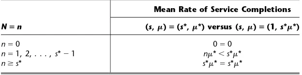
To understand why this result holds, consider any other solution to model 2, (s,)⫽(s*,*), where s*⬎1. The service capacity of this system (as measured by the mean rate of service completions when all servers are working) is s**. We shall now compare this solution with the corresponding single-server solution (s, )⫽(1, s**) having the sameservice capacity. In particular, Table 26.3 compares the mean rate at which
for CRAB computer for MBI computer. 3,750⫹2,640⫽$6,390 per day
5,000⫹1,160⫽$6,160 per day
1There also are minor restrictions on the queueing model and the waiting-cost function. However, any of the
service completions occur for each given number of customers in the system N⫽n. This table shows that the service efficiency of the (s*, *) solution sometimes is worse but never is better than for the (1,s**) solution because it can use the full service capacity only when there are at least s* customers in the system, whereas the single-server solu-tion uses the full capacity whenever there are anycustomers in the system. Because this lower service efficiency can only increase waiting in the system,E(WC) must be larger for (s*,*) than for (1,s**). Furthermore, the expected service cost must be at least as large because condition 2 [and f(0)⫽0] implies that
f(*)sⱖf(s**).
Therefore,E(TC) is larger for (s*,*) than (1,s**). Finally, note that condition 1 im-plies that there is a feasible solution with s⫽1 that is at least as good as (1,s**). The conclusion is that any s⬎1 solution cannotbe optimal for model 2, so s⫽1 must be optimal.1
This result is still of some use even when one or both conditions fail to hold. If cannot be made sufficiently large to permit a single server, it still suggests that a fewfast servers should be preferred to many slow ones. If condition 2 does not hold, we still know that E(WC) is minimized by concentrating any given amount of service capacity into a single server, so the best s⫽1 solution must be at least nearly optimal unless it causes a
substantial increase in service cost.
Model 3—Unknown and s
Model 3 is designed especially for the case where it is necessary to select both the num-ber of service facilitiesand the number of servers sat each facility. In the typical situa-tion, a population (such as the employees in an industrial building) must be provided with a certain service, so a decision must be made as to what proportion of the population (and therefore what value of ) should be assigned to each service facility. Examples of such facilities include employee facilities (drinking fountains, vending machines, and rest-rooms), storage facilities, and reproduction equipment facilities. It may sometimes be clear that only a single server should be provided at each facility (e.g., one drinking fountain or one copy machine), but soften is also a decision variable.
26.4 DECISION MODELS 26-13
■ TABLE 26.3 Comparison of service efficiency for Model 2 solutions
Mean Rate of Service Completions
Nⴝn (s, )ⴝ(s*, *) versus (s, )ⴝ(1, s**)
n⫽0 0⫽0
n⫽1, 2, . . . , s*⫺1 n*⬍s**
nⱖs* s**⫽s**
1For a rigorous proof of this result, see S. Stidham, Jr., “On the Optimality of Single-Server Queueing Systems,”
Operations Research,18:708–732, 1970. This result focuses on minimizing E(TC) when E(WC) is based on
waiting time in the system. However, if waiting costs are incurred only while waiting in the queue, markedly dif-ferent results occur. For example, see X. Chao and C. Scott, “Several Results on the Design of Queueing
Sys-tems,”Operations Research,48:965–970, 2000. Furthermore, even when waiting time in the system is the
rel-evant quantity, if the concern is to avoid extremely long waiting times as much as possible rather than minimizing
E(TC), then several slow servers become superior to one fast server when the service-time distribution is so
highly variable that it possesses some infinite higher moments. For an analysis of this alternative viewpoint, see A. Scheller-Wolf, “Necessary and Sufficient Conditions for Delay Moments in FIFO Multiserver Queues
To simplify our presentation, we shall require in model 3 that and sbe the same for all service facilities. However, it should be recognized that a slight improvement in the indicated solution might be achieved by permitting minor deviations in these param-eters at individual facilities. This should be investigated as part of the detailed analysis that generally follows the application of the mathematical model.
Formulation of Model 3.
Definitions: Cs⫽marginal cost of server per unit time.
Cf⫽fixed cost of service per service facility per unit time. p⫽mean arrival rate for entire calling population.
n⫽number of service facilities⫽p/. Given: ,Cs,Cf,p.
To find: ,s.
Objective: Minimize E(TC), subject to ⫽p/n, where n⫽1, 2, . . . .
Finding E(TC). It might appear at first glance that the appropriate expression for the expected total cost per unit time of all the facilities should be
E(TC)ⱨn[(Cf⫹Css)⫹E(WC)],
where E(WC) here represents the expected waiting cost per unit time for each facility. However, if this expression actually were valid, it would imply that n⫽1 necessarilyis optimal for model 3. The reasoning is completely analogous to that for the optimality of a single-server result for model 2; namely, any solution (n,s)⫽(n*,s*) with n*⬎1 has higher service costs than the (n,s)⫽(1,n*s*) solution, and it alsohas a higher expected waiting cost because it sometimes makes less effective use of the available service ca-pacity. In particular, it sometimes has idle servers at one facility while customers are wait-ing at another facility, so the mean rate of service completions would be less than if the customers had access to allthe servers at one common facility.
Because there are many situations where it obviously would notbe optimal to have just one service facility (e.g., the number of restrooms in a 50-story building), something must be wrong with this expression. Its deficiency is that it considers only the cost of service and the cost of waiting at the service facilitieswhile totally ignoring the cost of the time wasted in travelingto and from the facilities. Because travel time would be prohibitive with only one service facility for a large population, enough separate facilities must be distributed throughout the calling population to hold travel time down to a reasonable level.
Thus, letting the random variable Tbe the round-trip travel time for a customer com-ing to and gocom-ing back from one of the service facilities, we see that the total time lost by the customer actually is ᐃ⫹T. (Recall from Chap. 17 that ᐃis the waiting time in the queueing system after the customer arrives.) Therefore, a customer’s totalcost for time lost should be based on ᐃ⫹Trather than just ᐃ. To simplify the analysis, let us sepa-rate this total cost into the sum of the waiting-time cost based on ᐃ(or N) and the travel-time cost based on T. We shall also assume that the travel-time cost is proportional to T, where Ctis the cost of each unit of travel time for each customer. For ease of presenta-tion, suppose that the probability distribution of Tis the same for each service facility, so that CtE(T) is the expected travel costfor each arrival at any of the service facilities. The resulting expression for E(TC) is
E(TC)⫽n[(Cf⫹Css)⫹E(WC)⫹CtE(T)]
the overall minimum. The next section discusses how to evaluate E(T) and also solves an example (Example 3 of Sec. 26.1) fitting model 3.
26.5 THE EVALUATION OF TRAVEL TIME 26-15
■
26.5
THE EVALUATION OF TRAVEL TIME
As discussed in Sec. 26.4, one of the important considerations for deciding how many service facilities to provide is the amount of time that customers must spend traveling to and from a facility. Therefore,the expected round-trip travel time E(T) for a customer is one of the components of the objective function for model 3, the decision model that is concerned with deciding on the number of service facilities. We now shall elaborate on how to determine E(T).
E(T) can be interpreted as the average travel timespent by customers in coming both to and from a given service facility. Therefore, the value of E(T) depends very much upon the characteristics of the individual situation. However, we shall illustrate a rather general approach to evaluating E(T) by developing a basic travel-time model and then calculat-ing E(T) for the more complicated situation involved in Example 3. In both cases it is as-sumed that the portion of the population assigned to the service facility under considera-tion is distributed uniformlythroughout the assigned area, that each arrival returns to its original locationafter receiving service, and that the average speed of travel does not de-pend upon the distance traveled. Another basic assumption is that all travel is rectilinear, i.e., it progresses along a system of orthogonalpaths (aisles, streets, highways, and so on) that are parallelto the main sides of the area under consideration.
A Basic Travel-Time Model
Description: Rectangular area and rectilinear travel, as shown in Fig. 26.7.
Definitions: T⫽travel time (round trip) for an arrival.
v⫽average velocity (speed) of customers in traveling to and from facility.
a,b,c,d⫽respective distances from facility to boundary of area assigned to facility, as shown in Fig. 26.7.
Given: v,a,b,c,d.
To find: Expected value of T, E(T).
Using an orthogonal (x,y) coordinate system, Fig. 26.7 shows the coordinates (x,y) of the location of a particular customer. The xand ycoordinates of the location from which a random arrival comes actually are random variables Xand Y, where X ranges from ⫺ato cand Yranges from ⫺bto d. Because the total round-trip distance traveled by the random arrival is
D⫽2(|X|⫹|Y|)
(−a, −b)
(0, 0)
(c, d) (x, y)
■ FIGURE 26.7
and
T⫽ ᎏD vᎏ,
it follows that
E(T)⫽ ᎏ2
vᎏ(E{|X|}⫹E{|Y|}).
Thus, the problem is reduced to identifying the probability distributions of |X|and |Y|and then calculating their means.
First consider |X|. Its probability distribution can be obtained directly from the
dis-tribution of X. Because the customers are assumed to be distributed uniformly through-out the assigned area, and because the height of the rectangular area is the samefor all possible values of X⫽x,Xmust have a uniform distributionbetween ⫺a and c,as shown in Fig. 26.8a. Because |x|⫽|⫺x|, adding the probability density function values at xand
⫺xthen yields the probability distribution of |X|shown in Fig. 26.8b. Therefore, noting that |x|⫽x for x ⱖ0,
E{|X|}⫽
max{a,c}
0
x f|x|(x) dx
⫽
min{a,c}
0 ᎏa
2
⫹ x c ᎏdx⫹
max{a,c}
min{a,c} ᎏa⫹
x c ᎏdx
⫽ ᎏ1
2ᎏ ᎏa⫹
1
c
ᎏ[(min{a,c})2⫹(max{a,c})2]
⫽ ᎏ 2 a ( 2 a ⫹ ⫹ c c 2 ) ᎏ.
The analysis for |Y|is completely analogous, where the widthof the rectangular area for possible values of Y⫽ynow determines the probability distribution of Y.
The result is that
E{|Y|}⫽ ᎏ 2 b ( 2 b ⫹ ⫹ d d 2 ) ᎏ. Consequently,
E(T)⫽ ᎏ1
vᎏ
ᎏ a a 2 ⫹ ⫹ c c 2ᎏ ⫹ ᎏbb
2 ⫹ ⫹ d d 2 ᎏ
. 1a + c a + 1c
2 a + c
fx(x)
−a 0 c x 0 x
fx(x)
mina, c
maxa, c
(a) (b)
■ FIGURE 26.8
Example 3—How Many Tool Cribs? For the new plant being designed for the MECHANICAL COMPANY (see Sec. 26.1), the layout of the portion of the factory area where the mechanics will work is shown in Fig. 26.9. The three possiblelocations for tool cribs are identified as Locations 1, 2, and 3, where access to these locations will be pro-vided by a system of orthogonal aisles parallel to the sides of the indicated area. The co-ordinates are given in units of feet. The mechanics will be distributed quite uniformly throughout the area shown, and each mechanic will be assigned to the nearesttool crib. It is estimated that the mechanics will walk to and from a tool crib at an average speed of slightly less than 3 miles/hour, so vis set at v⫽15,000 feet/hour.
The three basic alternatives being considered are
Alternative 1: Have threetool cribs—use Locations 1, 2, and 3; Alternative 2: Have onetool crib—use Location 2;
Alternative 3: Have twotool cribs—use Locations 1 and 3.
The calculation of E(T) for each alternative is given next, followed by the use of model 3 to make the choice among them.
Alternative 1(n⫽3): If all three locations were used,eachtool crib would service a 300⫻
300 foot squarearea. Therefore, this case is just a special case of the basic travel-time model just presented, where a⫽c⫽150 and b⫽d⫽150. Consequently,
E(T)⫽ ᎏ
15,00 1
0 ft/hrᎏ
ᎏ 11 5 5
0 0
2
⫹ ⫹
1 1 5 5 0 0
2
ᎏ ⫹ ᎏ1
1 5 5
0 0
2
⫹ ⫹
1 1 5 5 0 0
2
ᎏ
ft⫽ ᎏ
15,00 1
0 ft/hrᎏ(300 ft)
⫽0.02 hr.
26.5 THE EVALUATION OF TRAVEL TIME 26-17
(0, 300) (300, 300)
(300, 600) (600, 600)
Location 3
(450, 450)
Location 2
(450, 150) Location 1
(150, 150)
(0, 0) (600, 0)
■ FIGURE 26.9
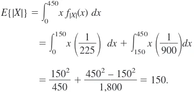
Alternative 2 (n⫽1):With just onetool crib (in Location 2) to service the entire area shown in Fig. 26.9, the derivation of E(T) is a little more complicated than it is for the basic travel-time model. The first step is to relabel Location 2 as the original (0, 0) for an (x,y) coordi-nate system, so that 450 would be subtracted from the first coordicoordi-nates shown and 150 would be subtracted from the second coordinates. The probability density function for Xis then ob-tained by dividing the heightfor each possible value of X⫽xby the total area (so that the area under the probability density function curve equals 1), as given in Fig. 26.10a. Combin-ing the values for xand ⫺xthen yields the probability distribution of |X|shown in Fig. 26.10b.
Hence,
E{|X|}⫽
450
0
x f|X|(x) dx
⫽
150
0
x
ᎏ2 1
25ᎏ dx⫹
450
150
x
ᎏ9 1 00ᎏ
dx⫽ ᎏ1
4 5
5 0
0
2
ᎏ ⫹ ᎏ450
1
2
,8 – 0
1 0
502
ᎏ ⫽150.
We suggest that you now try the same approach (using the width of the area rather than the height) to derive E{|Y|}. You will find that the probability distribution of Yis
identicalto that for |X|, so E{|Y|}⫽150. As a result,
E(T)⫽ ᎏ 15, 2
000ᎏ(150⫹150)
⫽0.04 hr.
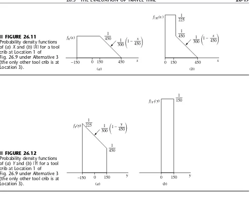
Alternative 3 (n⫽2):With tool cribs in just Locations 1 and 3, the areas assigned to them would be divided by a line segment between (300, 300) and (600, 0) in Fig. 26.9. Notice that the two areas and their tool cribs are located symmetrically with respect to this line segment. Therefore,E(T) is the same for both, so we shall derive it just for the tool crib in Location 1. (You might try it for the other tool crib for practice—see Prob. 26.5-3.) Proceeding just as for Alternative 2, relabel Location 1 as the origin (0, 0) for an (x,y) coordinate system, so that 150 would be subtracted from all coordinates shown in Fig. 26.9. This relabeling leads directly to the probability density function of X, and then of |X|, shown
in Fig. 26.11. As a result,
1 450
1 900 fX(x)
−450 −150 x x
(a) 0 150
1 225
1 900
450 fX(x)
(b) 0 150
■ FIGURE 26.10
E{|X|}⫽ ᎏ 2 1 25ᎏ
150 0x dx⫹ ᎏ
3 1 00ᎏ
450
150
1 –ᎏ 45
x
0
ᎏ
x dx⫽ ᎏ
2 1 25ᎏ
ᎏx 2 2 ᎏ
0 150 ⫹ ᎏ 3 1 00ᎏᎏx 2 2 ᎏ– ᎏ 1, x 3 3 50 ᎏ
450 150 ⫽ ᎏ 2 1 25ᎏ ᎏ15 2 02 ᎏ ⫹ ᎏ 3 1 00ᎏ
ᎏ45 2 02 ᎏ– ᎏ 1 4 , 5 3 0 5 3 0 ᎏ
– ᎏ 3 1 00ᎏᎏ15 2 02 ᎏ– ᎏ 1 1 , 5 3 0 5 3 0 ᎏ
⫽133ᎏ1 3ᎏ.
Next, the probability density function ofYis obtained by using the widthof the area assigned to the tool crib at Location 1 for each possible value of Y⫽yand then dividing by the size of the area, as given in Fig. 26.12a. This result then yields the uniform distri-bution of |Y|shown in Fig. 26.12b. Thus,
E{|Y|}⫽ ᎏ
1 1 50ᎏ
150 0 y dy ⫽75.26.5 THE EVALUATION OF TRAVEL TIME 26-19
x 1 225 1 450 450 fX(x)
(b)
0 150
1 300
x 450
1 −
1 450 fX(x)
−150 x
(a)
0 150 450
1 300
x 450
1 −
■ FIGURE 26.11
Probability density functions of (a) Xand (b) |X| for a tool crib at Location 1 of Fig. 26.9 under Alternative 3 (the only other tool crib is at Location 3).
1 450 1
225 fY(y)
−150
(a)
0 150
1 300
y 450
1 −
y
fY(y)
(b) 1 150
0 150 y
■ FIGURE 26.12
Consequently,
E(T)⫽ ᎏ 15, 2
000ᎏ(133ᎏ 1 3ᎏ⫹75)
⫽0.0278 hr.
Applying Model 3:Because E(T) now has been evaluated for the three alternatives under consideration, the stage is set for using model 3 from Sec. 18.4 to choose among these alternatives. Most of the data required for this model are given in Sec. 26.1, namely,
⫽120 per hour, Cf⫽$16 per hour, Cs⫽$20 per hour, p⫽120 per hour, Ct⫽$48 per hour,
where the M/M/smodel given in Sec. 17.6 is used to calculate Land so on. In addition, the end of Sec. 26.3 gives E(WC)⫽48Lin dollars per hour. Therefore,
E(TC)⫽n
(16⫹20s)⫹48L⫹ ᎏ12 n0
ᎏ48E(T)
.The resulting calculation of E(TC) for various svalues for each nis given in Table 26.4, which indicates that the overall minimum E(TC) of $295.20 per hour is obtained by hav-ing three tool cribs (so ⫽40 for each), with one clerk at each tool crib.
■
26.6
CONCLUSIONS
■ TABLE 26.4 Calculation of E(TC), in dollars per hour for Example 3
n s L E(T) CfⴙCss E(WC) CtE(T) E(TC)
1 120 1 ⴥ 0.0400 $36 ⴥ $230.40 ⴥ
1 120 2 1.333 0.0400 $56 $64.00 $230.40 $350.40
1 120 3 1.044 0.0400 $76 $50.11 $230.40 $356.51
2 60 1 1.000 0.0278 $36 $48.00 $ 80.00 $328.00
2 60 2 0.534 0.0278 $56 $25.63 $ 80.00 $323.26
3 40 1 0.500 0.0200 $36 $24.00 $ 38.40 $295.20
3 40 2 0.344 0.0200 $56 $16.51 $ 38.40 $332.73
This chapter has discussed the application of queueing theory for designingqueueing sys-tems. Every individual problem has its own special characteristics, so no standard proce-dure can be prescribed to fit every situation. Therefore, the emphasis has been on introducing fundamental considerations and approaches that can be adapted to most cases. We have fo-cused on three particularly common decision variables (s,, and ) as a vehicle for intro-ducing and illustrating these concepts. However, there are many other possible decision variables (e.g., the size of a waiting room for a queueing system) and many more compli-cated situations (e.g., designing a priorityqueueing system) that can also be analyzed in a similar way.
To the left of each of the following problems (or their parts), we have inserted a T whenever one of the templates for this chapter (and Chap. 17) can be useful.
26.2-1. For each kind of queueing system listed in Prob. 17.3-1, briefly describe the nature of the cost of serviceand the cost of waitingthat would need to be considered in designing the system.
26.3-1. Suppose that a queueing system fits the M/M/1 model de-scribed in Sec. 17.6, with ⫽2 and ⫽4. Evaluate the expected waiting cost per unit time E(WC) for this system when its waiting-cost function has the form
(a) g(N)⫽10N⫹2N2.
(b) h(ᐃ)⫽25ᐃ⫹ᐃ3.
26.3-2. Follow the instructions of Prob. 26.3-1 for the following waiting-cost functions.
(a) g(N)⫽
(b) h(ᐃ)⫽
for 0 ⱕᐃⱕ1forᐃⱖ1. ᐃ
ᐃ2
forN⫽0, 1, 2 forN⫽3, 4, 5 forN⬎5. 10N
6N2 N3
PROBLEMS 26-21
determining the numberof service facilities to provide when customersmust travel to the nearest facility. But travel-time models also can be very useful when the servers must travel to the customer from the service facility (e.g., fire trucks and ambulances), as well as in other contexts.
Another useful area for the application of queueing theory is the development of poli-cies for controllingqueueing systems, e.g., for dynamicallyadjusting the number of servers or the service rate to compensate for changes in the number of customers in the system. Research is being conducted in this area.
Queueing theory has proved to be a very useful tool, and we anticipate that its use will continue to grow as recognition of the many guises of queueing systems grows.
■
SELECTED REFERENCES
■
LEARNING AIDS FOR THIS CHAPTER ON CD-ROM
■
PROBLEMS
1. Allen, A. O.:Probability, Statistics, and Queueing Theory with Computer Science Applications,
2d ed., Academic Press, New York, 1990, chaps. 5–6.
2. Hall, R. W.:Queueing Methods: For Services and Manufacturing,Prentice-Hall, Upper Saddle River, NJ, 1991.
3. Hillier, F. S., and M. S. Hillier:Introduction to Management Science: A Modeling and Case Stud-ies Approach with Spreadsheets, McGraw-Hill/Irwin, Burr Ridge, IL, 2d ed., 2003, chap. 14.
4. Kleinrock, L.:Queueing Systems, vol. II: Computer Applications,Wiley, New York, 1976.
5. Lee, A. M.:Applied Queueing Theory,St. Martin’s Press, New York, 1966.
6. Newell, G. F.:Applications of Queueing Theory,2d ed., Chapman and Hall, London, 1982.
7. Nordgren, B.: “The Problem with Waiting Times,”IIE Solutions,May 1999, pp. 44–48.
8. Papadopoulos, H. T., C. Heavey, and J. Browne:Queueing Theory in Manufacturing Systems Analysis and Design,Chapman and Hall, London, 1993.
9. Stidham, S., Jr.: “Analysis, Design, and Control of Queueing Systems,”Operations Research,
50:197–216, 2002.
Excel Files:
Same templates as provided for Chap. 17
“Ch. 26—Application of QT” LINGO File for Selected Examples
26.4-1. A certain queueing system has a Poisson input, with a mean arrival rate of 4 customers per hour. The service-time distri-bution is exponential, with a mean of 0.2 hour. The marginal cost of providing each server is $20 per hour, where it is estimated that the cost that is incurred by having each customer idle(i.e., in the queueing system) is $120 per hour for the first customer and $180 per hour for each additional customer. Determine the number of servers that should be assigned to the system to minimize the ex-pected total cost per hour. [Hint:Express E(WC) in terms of L,P0,
and , and then use Figs. 17.6 and 17.7.]
26.4-2. Reconsider Prob. 17.6-9. The total compensation for the new employee would be $8 per hour, which is just half that for the cashier. It is estimated that the grocery store incurs lost profit due to lost future business of $0.08 for each minute that each customer has to wait (including service time). The manager now wants to determine on an expected total cost basis whether it would be worthwhile to hire the new person.
(a) Which decision model presented in Sec. 26.4 applies to this problem? Why?
(b) Use this model to determine whether to continue the status quo or to adopt the proposal.
26.4-3. The Southern Railroad Company has been subcontracting for the painting of its railroad cars as needed. However, manage-ment has decided that the company can save money by doing this work itself. A decision now needs to be made to choose between two alternative ways of doing this.
Alternative 1 is to provide two paint shops, where painting is done by hand (one car at a time in each shop), for a total hourly cost of $70. The painting time for a car would be 6 hours. Alter-native 2 is to provide one spray shop involving an hourly cost of $100. In this case, the painting time for a car (again done one at a time) would be 3 hours. For both alternatives, the cars arrive ac-cording to a Poisson process with a mean rate of 1 every 5 hours. The cost of idle time per car is $100 per hour.
(a) Use Fig. 17.9 to estimate L,Lq,W, and Wqfor Alternative 1.
(b) Find these same measures of performance for Alternative 2.
(c) Determine and compare the expected total cost per hour for these alternatives.
26.4-4. The production of tractors at the Jim Buck Company in-volves producing several subassemblies and then using an assem-bly line to assemble the subassemblies and other parts into finished tractors. Approximately three tractors per day are produced in this way. An in-process inspection station is used to inspect the sub-assemblies before they enter the assembly line. At present there are two inspectors at the station, and they work together to inspect each subassembly. The inspection time has an exponential distribution, with a mean of 15 minutes. The cost of providing this inspection system is $40 per hour.
A proposal has been made to streamline the inspection proce-dure so that it can be handled by only one inspector. This inspector would begin by visually inspecting the exterior of the subassembly, and she would then use new efficient equipment to complete the in-spection. Although this process with just one inspector would slightly
increase the mean of the distribution of inspection times from 15 minutes to 16 minutes, it also would reduce the variance of this distribution to only 40 percent of its current value.
The subassemblies arrive at the inspection station according to a Poisson process at a mean rate of 3 per hour. The cost of hav-ing the subassemblies wait at the inspection station (thereby in-creasing in-process inventory and possibly disrupting subsequent production) is estimated to be $20 per hour for each subassembly. Management now needs to make a decision about whether to continue the status quo or adopt the proposal.
T (a) Find the main measures of performance—L,Lq,W,Wq—for
the current queueing system.
(b) Repeat part (a) for the proposed queueing system.
(c) What conclusions can you draw about what management should do from the results in parts (a) and (b)?
(d) Determine and compare the expected total cost per hour for the status quo and the proposal.
26.4-5. The car rental company, Try Harder, has been subcon-tracting for the maintenance of its cars in St. Louis. However, due to long delays in getting its cars back, the company has decided to open its own maintenance shop to do this work more quickly. This shop will operate 42 hours per week.
Alternative 1 is to hire two mechanics (at a cost of $1,500 per week each), so that two cars can be worked on at a time. The time required by a mechanic to service a car has an Erlang distribution, with a mean of 5 hours and a shape parameter of k⫽8.
Alternative 2 is to hire just one mechanic (for $1,500 per week) but to provide some additional special equipment (at a cap-italized cost of $1,250 per week) to speed up the work. In this case, the maintenance work on each car is done in two stages, where the time required for each stage has an Erlang distribution with the shape parameter k⫽4, where the mean is 2 hours for the first stage and 1 hour for the second stage.
For both alternatives, the cars arrive according to a Poisson process at a mean rate of 0.3 car per hour (during work hours). The company estimates that its net lost revenue due to having its cars unavailable for rental is $150 per week per car.
(a) Use Fig. 17.11 to estimate L,Lq,W, and Wqfor alternative 1.
(b) Find these same measures of performance for alternative 2.
(c) Determine and compare the expected total cost per week for these alternatives.
26.4-6. A certain small car-wash business is currently being ana-lyzed to see if costs can be reduced. Customers arrive according to a Poisson process at a mean rate of 15 per hour, and only one car can be washed at a time. At present the time required to wash a car has an exponential distribution, with a mean of 4 minutes. It also has been noticed that if there are already 4 cars waiting (in-cluding the one being washed), then any additional arriving cus-tomers leave and take their business elsewhere. The lost incre-mental profit from each such lost customer is $6.
PROBLEMS 26-23
longer than ᎏ12ᎏhour (according to a time slip she receives upon
ar-rival) before her car is ready, then she receives a free car wash (at a marginal cost of $4 for the company). This guarantee would be well posted and advertised, so it is believed that no arriving cus-tomers would be lost.
Proposal 2 is to obtain the most advanced equipment avail-able, at an increased cost of $20 per hour, and each car would be sent through two cycles of the process in succession. The time re-quired for a cycle has an exponential distribution, with a mean of 1 minute, so total expected washing time would be 2 minutes. Be-cause of the increased speed and effectiveness, it is believed that essentially no arriving customers would be lost.
The owner also feels that because of the loss of customer goodwill (and consequent lost future business) when customers have to wait, a cost of $0.20 for each minute that a customer has to wait before her car wash begins should be included in the analy-sis of all alternatives.
Evaluate the expected total cost per hour E(TC) of the status quo, proposal 1, and proposal 2 to determine which one should be chosen.
26.4-7. The Seabuck and Roper Company has a large warehouse in southern California to store its inventory of goods until they are needed by the company’s many furniture stores in that area. A sin-gle crew with four members is used to unload and/or load each truck that arrives at the loading dock of the warehouse. Manage-ment currently is downsizing to cut costs, so a decision needs to be made about the future size of this crew.
Trucks arrive at the loading dock according to a Poisson process at a mean rate of 1 per hour. The time required by a crew to unload and/or load a truck has an exponential distribution (re-gardless of crew size). The mean of this distribution with the four-member crew is 15 minutes. If the size of the crew were to be changed, it is estimated that the mean service rate of the crew (now
⫽4 customers per hour) would be proportional to its size. The cost of providing each member of the crew is $20 per hour. The cost that is attributable to having a truck not in use (i.e., a truck standing at the loading dock) is estimated to be $30 per hour.
(a) Identify the customers and servers for this queueing system. How many servers does it currently have?
T (b) Use the appropriate Excel template to find the various mea-sures of performance for this queueing system with four members on the crew. (Set t⫽1 hour in the Excel template for the waiting-time probabilities.)
T (c) Repeat (b) with three members.
T (d) Repeat part (b) with two members.
(e) Should a one-member crew also be considered? Explain.
(f ) Given the previous results, which crew size do you think man-agement should choose?
(g) Use the cost figures to determine which crew size would min-imize the expected total cost per hour.
(h) Assume now that the mean service rate of the crew is propor-tional to the square root of its size. What should the size be to minimize expected total cost per hour?
26.4-8. Trucks arrive at a warehouse according to a Poisson process with a mean rate of 4 per hour. Only one truck can be loaded at a time. The time required to load a truck has an expo-nential distribution with a mean of 10/nminutes, where nis the number of loaders (n⫽1, 2, 3, . . .). The costs are (i) $18 per hour for each loader and (ii) $20 per hour for each truck being loaded or waiting in line to be loaded. Determine the number of loaders that minimizes the expected hourly cost.
26.4-9. A company’s machines break down according to a Pois-son process at a mean rate of 3 per hour. Nonproductive time on any machine costs the company $60 per hour. The company em-ploys a maintenance person who repairs machines at a mean rate of machines per hour (when continuously busy) if the company pays that person a wage of $5per hour. The repair time has an exponential distribution.
Determine the hourly wage that minimizes the company’s to-tal expected cost.
26.4-10. Jake’s Machine Shop contains a grinder for sharpening the machine cutting tools. A decision must now be made on the speed at which to set the grinder.
The grinding time required by a machine operator to sharpen the cutting tool has an exponential distribution, where the mean 1/can be set at 0.5 minute, 1 minute, or 1.5 minutes, depend-ing upon the speed of the grinder. The runndepend-ing and maintenance costs go up rapidly with the speed of the grinder, so the esti-mated cost per minute is $1.60 for providing a mean of 0.5 minute, $0.40 for a mean of 1.0 minute, and $0.20 for a mean of 1.5 minutes.
The machine operators arrive randomly to sharpen their tools at a mean rate of 1 every 2 minutes. The estimated cost of an op-erator being away from his or her machine to the grinder is $0.80 per minute.
T (a) Obtain the various measures of performance for this queue-ing system for each of the three alternative speeds for the grinder. (Set t⫽5 minutes in the Excel template for the wait-ing time probabilities.)
(b) Use the cost figures to determine which grinder speed mini-mizes the expected total cost per minute.
26.4-11. Consider the special case of model 2 where (1) any
<