Optimization of the Fuzzy Logic Controller for an Autonomous UAV
Jon C. Ervin Apogee Research Group
LosOsos, CA 93402 [email protected]
Sema E. Alptekin California Polytechnic State
University
San Luis Obispo, CA 93407, USA [email protected]
Dianne J. DeTurris California Polytechnic State
University
San Luis Obispo, CA 93407, USA [email protected]
Abstract
In this paper, we describe the optimization of membership functions in an application employing a hierarchical Fuzzy Logic Controller. The size of the rule base is made manageable by using a unique formulation, known as Combs method, to help control the problem of ‘exponential rule expansion’. The optimization is performed using a steady state genetic algorithm with a dynamic fitness function. The controller being developed is designed to fly a small, autonomous parafoil, suitable for short-range reconnaissance and land survey applications. The optimization process is performed in the Matlab/Simulink software environment and incorporates fuzzy logic modules developed in the Matlab Fuzzy Logic Toolbox. Hardware limitations in terms of memory, computational speed and cost were critical factors driving the need for this simple yet robust control algorithm.
Keywords: Genetic Algorithms, Fuzzy Logic.
1 Introduction
Using Genetic Algorithms (GA) to optimize the performance of a Fuzzy Logic Controller (FLC) has been the focus of a number of research efforts [1-8]. The approach taken in this application combines various techniques explored in previous research efforts. The FLC produced in this research was specifically designed to provide autonomous guidance for a short range, unmanned air vehicle
(UAV). The main hardware elements of the Autonomous Tactical Reconnaissance Platform (ATRP) are a 3.5 square meter parafoil, an electronics payload with a protective aerodynamic housing and a launch system.
In order to keep product costs to a minimum, inexpensive electronic components were used to provide inputs to the controller software. A fuzzy logic control method is employed in the ATRP for its advantages in fault tolerance and graceful response to missing and/or noisy sensor input. One of the major drawbacks to fuzzy control is the exponential growth in the number of rules as the number of input variables increases linearly. A unique methodology (Combs’ method) is used to address this problem of ‘exponential rule expansion’ [9]. The use of Combs’ method also simplified the tuning process of the fuzzy system by requiring only the optimization of the membership functions and not the rule base. Modularity and simplicity of design were further enhanced by adopting a hierarchical fuzzy logic architecture.
the candidate solution. The process then repeats itself until a satisfactory result is obtained.
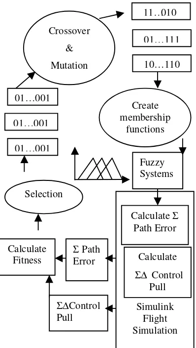
Figure 1. Block Diagram of GA based optimization
The optimization process is performed entirely within the Matlab software environment. The same Matlab/Simulink simulated flight plan with randomized environmental conditions is used to evaluate the fitness of each candidate solution in the GA population.
In Section 2, we provide a brief background on Fuzzy Control and Combs method. Development of the Fuzzy Logic Architecture for the ATRP application is presented in Section 3, followed by a discussion of the simulation and optimization of the control algorithm in Section 4. The hardware implementation of the concept is reported in Section 5 with conclusions and future work discussed in Section 6.
2 Fuzzy Control
A fuzzy logic control algorithm provides the autonomous decision making strategy for the ATRP. Attributes of fuzzy logic that made it appealing for this application are the ability to model nonlinear functions, robustness in the face of imprecise input and ease of code generation. Fuzzy logic algorithms are intuitively easy to understand and allow the user to encapsulate the experience of experts in an efficient manner. References cited at the end of this article can give the reader a much more comprehensive insight into fuzzy logic fundamentals [10-12].
One of the well documented disadvantages of the fuzzy logic algorithm is known as “exponential rule expansion”. In general, each input variable has a number of associated fuzzy membership functions. In the simplest approach to building a rule base, a separate rule is formed for each of the possible combinations of the input membership functions. A 2 input - 1 output system with 3 membership functions each would have 32 = 9 rules in this type of rule base. This system of rules works well for a small two input problem, but as the number of inputs and/or corresponding membership functions increases linearly, the number of rules increases exponentially. Usually an attempt is made to reduce the number of rules either by eliminating those rules that would not be encountered in the operating environment or in some way limiting the number of membership functions for each variable.
A method first developed by Combs allows us to avoid the exponential rule growth in favor of a much more manageable linear growth [9]. The main difference between the Combs’ formulation and that of the traditional method is that in Combs’ method every rule in the rule base has only one antecedent for every consequent. Each membership function of all the input variables is used once in the antecedent of a rule in the rule base. In the 2 input – 1 output example, the number of rules in the rule base is reduced to six versus nine for the traditional method. For a high speed controller, this difference would be trivial but a modest increase in the number of inputs and membership functions can soon lead to a very large rule base and an incredible reduction in rules using Combs method. To illustrate, suppose you have a fuzzy system of 5 inputs with 7 membership functions each, Combs method will have only 35 rules (5x7=35) rather than the 16,807 (75) rules of the conventional technique.
01…001
Calculate Fitness
01…111
10…110
Fuzzy Systems 01…001
01…001
Create membership
functions
Calculate Σ
Path Error
Calculate
Σ∆ Control Pull
Σ Path Error
Σ∆Control Pull Selection
Simulink Flight Simulation
11…010
Crossover
&
Using Combs’ method to construct rules also served to simplify the optimization process discussed in a later section of this paper. The optimization task was further simplified by predetermining the number of membership functions for each input variable. It was necessary to keep the number of membership functions to the barest possible minimum due to memory and speed constraints of the microcontroller. At the same time the demands of the control function required enough membership functions for each input to provide the flexibility needed to achieve good flight performance. A large number of simulation flights were performed, with varying environmental conditions, to empirically determine a reasonable number of membership functions for each variable. If the optimization had proven unable to develop a solution that met requirements then one option to consider would have been to increase the number of membership functions for at least some of the input variables.
There is a large body of research described in the literature on methods to modify membership functions in the optimization process. The technique followed in this application was to define an initial set of triangular membership functions for each variable. A simple scaling function of two independent variables was used for each input to modify the shape and location of the membership functions. The scaling function for each input variable has a proportional and an exponent term of the form;
F(x) = a x b (1)
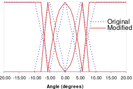
The proportional term “a” in (1) has the effect of varying the width and spacing of the membership functions evenly over the domain. The term in the exponent “b” produces a nonlinear spacing of membership functions and distorts the straight sides into curved line segments. The combination of the two terms provides good flexibility in modifying the membership functions without incurring a high computational overhead. Fig. 2 shows an example of the modification of membership functions that can be achieved with this scaling function.
The combined effect of the two scaling factors in this example is to widen the membership function centered at 0.0, push the peak of the middle membership functions out wider and pull the outermost membership functions inwards. Different combinations of values of the scaling functions will
have widely differing effects on the resulting modified membership functions. There is no provision in this approach for making asymmetric membership functions, however in this application it is hard to conceive of a scenario where asymmetry would be a desirable trait.
-20.00 -15.00 -10.00 -5.00 0.00 5.00 10.00 15.00 20.00
Angle (degrees)
Original Modified Orig X2
Figure 2. Membership Functions Before and After Modification (a = .4, b= 2.0)
A total of 14 scaling terms for the 7 variables (5 input and 2 output) of the two fuzzy logic modules make up the chromosome for the genetic algorithm optimization. These terms were limited to a range of values between .3 and 5.0. Values outside of these limits were found to be well outside the region for any optimal solution.
3 The Simulation Model
The flight simulation developed in Matlab/Simulink is used to evaluate candidate solutions passed from the optimization routine. The difference between the desired and actual heading (∆θ) along with the first and second derivatives of this difference are supplied to the Course Following fuzzy logic module. Any adjustments from the fuzzy Course Correction module are added to ∆θ and the controller uses these inputs to produce a control line pull command. The effect of the control line pull command on the aerodynamic performance of the parafoil is computed and an incremental parafoil heading vector is determined.
goal coordinates are used to compute the inputs for the fuzzy Course Correction module. The output from the Course Correction module completes the loop and the simulation runs for the length of an entire simulated mission profile
The two fuzzy logic sub-modules of the simulation serve as the brain for the autonomous controller. It is the membership functions for the input and output variables for each of these modules that are the focus of the optimization effort. The simulation parameters of wind strength, frequency of wind gusts, direction of wind and initial deploy heading are randomly altered during an optimization run after each generation has been computed.
4 Optimization Parameter Choices
A genetic algorithm (GA) was chosen as a convenient method to perform the optimization with a reasonable expectation of success. Genetic algorithms have proven effective in NP hard problems, they are easy to develop and code, and if properly designed they will avoid pitfalls that can trap other optimization techniques. Specifically, a Steady State Genetic Algorithm (SSGA) was chosen for this task as it was expected that this technique would simplify the task of computer code development.
An incremental SSGA is different from a more traditional GA in that only one member of the population of solutions is chosen for replacement at the end of each ‘generation’. One issue to be determined by the designer is how to select the member to be replaced. One obvious choice is to replace the worst performing member, but it has been reported that this can lead to premature convergence on a local optimum before the entire solution space can be explored. Another choice for replacement is to eliminate the oldest member in the population, but this technique runs the risk of losing the best performing solution. The technique used in this application was to replace the worst performing candidate while maintaining diversity through the application of a high mutation rate and a dynamic objective function.
There are also a variety of techniques that can be used in determining the parent or parents of the new candidate solution in each generation. Various means of selection include; Fitness Proportionate Selection with some form of associated scaling and windowing methods, Roulette Wheel Selection,
Rank Selection, and Tournament Selection [13]. A form of tournament selection, with five individuals randomly chosen from the population, was used for this application. Another choice to be made was whether to pick both parents from the random tournament or to use the best individual in the population as one parent and select the other from the tournament.
Random tournament selection to obtain both parents was the method used for all runs where the fitness function remained static throughout an optimization run. Eventually the optimization method of using a static fitness function was abandoned and with it the random selection of both parents was abandoned as well. When a dynamic fitness function, as described below, was incorporated into the optimization routine the elitist strategy of maintaining the best solution as one parent was adopted. The change in selection method was adopted based on the assumption that greater continuity in the generation of solutions would be required to obtain a feasible solution within a reasonable number of iterations. This assumption was not verified and remains as an interesting question for further research.
Another decision to be made in the construction of the SSGA is the type of cross-over to be employed. Cross-over, the exchange of sections of genetic material between parent solutions, can be limited to a single cut and swap operation as in single point cross-over or can occur at multiple locations on the chromosome. A special case of multi point crossover, uniform crossover, was implemented in this application with an equal chance of each bit being contributed by either parent. The mutation rate of .4, referred to in the literature as hypermutation, was chosen to ensure that the population did not become trapped at a local optima in the solution space.
Using an extraordinarily high mutation rate was expected to provide a more thorough search of the solution space at the cost of greatly increasing the number of iterations required for convergence. A compromise to this expected, though not empirically demonstrated, problem was to perform mutation using a Gaussian rather than uniform distribution.
path at each time step. There was also a desire that the magnitude of pull commands performed by the servo motors be minimized as much as possible. This desired trait was captured by summing the change in pull commands at each time step. The sum of these two error measures provided the fitness measure to be minimized in optimization efforts.
5 Results
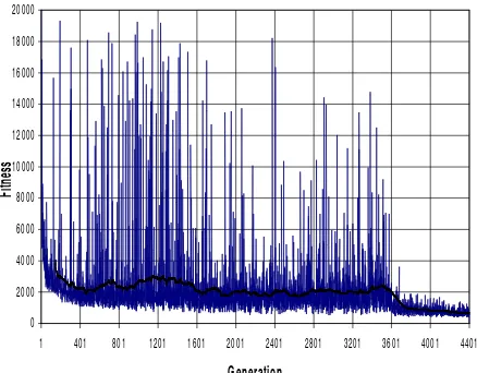
Fig. 3 and Fig. 4 show the results of running the SSGA optimization for 4,400 generations.
Figure 3. Fitness with the Mutation Rate Zeroed Out at Generation 3600
Figure 4. Constituent Values with Mutation Rate Zeroed Out at Generation 3600
The solid black line through the center of the data in figure 3 is a moving average of 144 values. Fig. 3 exhibits a noisy profile caused by the random choice of initial conditions for the simulation performed at
each generation. During the optimization process the initial environmental conditions for a particular generation may be relatively benign resulting in a good fitness score, whereas the following generation may be faced with a much more difficult set of initial conditions.
When the mutation rate is zeroed out at generation 3,600, the values of the individual genes eventually converged to a single value. The effect of this convergence resulted in a slight worsening of the average fitness over all values of environmental conditions. The optimization was allowed to continue to run for some time after convergence had occurred to ensure that no set of conditions would produce an unacceptable fitness value.
Fig. 5 shows the least fit candidates throughout the optimization run. Note that once the mutation rate has been zeroed out at generation 3600, the least fit candidates no longer show unacceptably high values.
Figure 5. Least Fit Solution at Each Generation
Maximum wind speed, wind direction, frequency of wind speed change, and initial course heading are the variables that had the greatest impact in determining the optimum fuzzy logic membership function values. The various initial conditions were changed randomly after each generation in the SSGA process.
6 Conclusions and Future Work
The optimization of a FLC using a Genetic Algorithm was a crucial element in the development of an autonomous UAV. The combination of using Combs Method to construct rules, using simulation
0 2000 4000 6000 8000 10000 12000 14000 16000 18000 20000
1 401 801 1201 1601 2001 2401 2801 3201 3601 4001 4401
Generation
Fi
tn
es
in the construction of the fitness function and making the fitness function dynamic in the GA optimization proved effective in achieving the desired controller properties.
The Combs method of formulating fuzzy rules proved to be a very effective means of minimizing the number of rules, resulting in tremendous savings in memory and execution speed. Although we cannot generalize our results to all fuzzy logic applications, the method seems to have merit for a number of applications where the “curse of exponential rule expansion” has been shown to be a limiting factor. The hierarchical organization of the fuzzy modules made for an easily understood and modifiable architecture. Future development may include adding additional modules to further enhance capability.
Throughout the optimization process decisions had to be made between several promising alternatives in order to proceed to the next step. A thorough examination of each alternative was not possible, so choices were made based on simplifying assumptions and prior experience.
The probability of mutation was chosen to be very high, reflecting the desire to ensure that the entire domain would be searched for candidate solutions. An interesting trade study could be performed to examine what effect that varying the mutation rate would have on solution convergence. Toward the end of the optimization run, specific scaling values were obtained by forcing the mutation rate to zero. Other methods, such as a least squared error analysis of candidate solutions might be expected to give better results. These are a few of many avenues of research that could be explored with respect to the assumptions and techniques used in this project.
References
[1] Tunstel E. and Mo Jamshidi, “On Genetic Programming of Fuzzy Rule-Based Systems for Intelligent Control”, International Jou rnal of Intelligent Automation and Soft Computing, Vol. 2, No. 3, p: 273-284, 1996.
[2] Cordon, O., F. Herrera, L. Magdalena, and P. Villar, “A Genetic LearningProcess for the Scaling Factors, Granularity and Contexts of the Fuzzy Rule-Based System Data Base, World Scientific, 2001.
[3] Maniadakis, M., S. Hartmut, “A Genetic Algorithm for Structural and Parametric Tuning
of Fuzzy Systems”, European Symposium on Intelligent Techniques, ESIT99.
[4] Hoffman, F., G. Pfister, “Evalutionary Design of a Fuzzy Knowledge Base for a Mobile Robot”, International Journal of Appropriate Reasoning, 11:1-158, 1994.
[5] Fukuda, T., N. Kubota, “An Intelligent Robotic System Based on a Fuzzy Approach”, Proceedings of the IEEE, Vol. 87, No. 9, September 1999.
[6] Tunstel E., T. Lippincott, and M. Jamshidi, , “Behaviour Hierarchy for Autonomous Mobile Robots: Fuzzy-behaviour Modulation and Evolution”, International Journal of Intelligent Automation and Soft Computing, Vol. 3, No. 1, pp. 37–50, 1997.
[7] Ghosh A., S. Tsutsui and H. Tanaka, “Function Optimization in Nonstationary Environment using Steady State Genetic Algorithms with Aging of Individuals, IEEE International Conference on Evolutionary Computation’98 . [8] Cordon O., F. Herrara, Hoffman, and L.
Magdalena, Genetic Fuzzy Systems – Evolutionary and Learning of Fuzzy Knowledge Bases, World Scientific, 2001.
[9] Combs, W.E., and J.E. Andrews, “Combinatorial Rule Explosion Eliminated by a Fuzzy Rule Configuration”, IEEE Transactions on Fuzzy Systems, Vol. 6, No. 1, pp. 1-11, 1998. [10] Jamshidi, M., A. Titli, L. A. Zadeh, and S.
Boverie, (Eds.), Applications of Fuzzy Logic, Prentice Hall, 1997.
[11] Zadeh, L.A., “Outline of a new approach to the analysis of complex systems and decision processes”, IEEE Trans. on Systems, Man and Cybernetics SMC-3, 28-44, 1973.
[12] Cox, E., The Fuzzy Systems Handbook: A Practitioner’s Guide to Building, Using, and Maintaining Fuzzy Systems, Academic, Boston, MA, 1994.
[13] Hancock, P., “An Empirical Comparison of Selection Methods in Evolutionary Algorithms”, printed in the Proceedings of the AISB Workshop on Evolutionary Computation, 1994.
Acknowledgments