Phase Space of Rolling Solutions of the Tippe Top
⋆S. Torkel GLAD †, Daniel PETERSSON † and Stefan RAUCH-WOJCIECHOWSKI ‡
† Dept. of Electrical Engineering, Link¨opings Universitet SE-581 83 Link¨oping, Sweden E-mail: [email protected], [email protected]
‡ Department of Mathematics, Link¨opings Universitet, SE-581 83 Link¨oping, Sweden E-mail: [email protected]
Received September 15, 2006, in final form February 05, 2007; Published online March 09, 2007 Original article is available athttp://www.emis.de/journals/SIGMA/2007/041/
Abstract. Equations of motion of an axially symmetric sphere rolling and sliding on a plane are usually taken as model of the tippe top. We study these equations in the nonsliding regime both in the vector notation and in the Euler angle variables when they admit three integrals of motion that are linear and quadratic in momenta. In the Euler angle variables (θ, ϕ, ψ) these integrals give separation equations that have the same structure as the equa-tions of the Lagrange top. It makes it possible to describe the whole space of soluequa-tions by representing them in the space of parameters (D, λ, E) being constant values of the integrals of motion.
Key words: nonholonomic dynamics; rigid body; rolling sphere; tippe top; integrals of motion
2000 Mathematics Subject Classification: 70E18; 70E40; 70F25; 70K05
1
Introduction
The tippe top (TT) has the shape of a truncated sphere with a knob. The tippe top is well known for its counterintuitive behavior that after being launched with sufficiently fast spin it turns upside down to spin on the knob until loss of energy makes it fall down again onto the spherical bottom.
It is well known now that the sliding friction is the only force producing a vertical component of the torque, which is needed for reducing the vertical component of the spin and for transferring the rotational energy into the potential energy by raising the center of mass (CM) and inverting the tippe top.
Equations describing rolling motions of an axially symmetric sphere are a limiting case of the TT equations and their solutions cannot display the TT rising phenomenon since the sliding friction is absent. They do, however indicate how solutions of the TT equations with weak friction behave in shorter time periods. According to experiments and numerical simulations [4, 5,1] the rising of CM of TT has a wobbly character which means that the inclination angle of the symmetry axisθ(t) is rising in an oscillatory manner. The analysis of the purely rolling solutions presented here supports an understanding that rising of CM may be seen as a superposition of a generic nutational motion of a rolling sphere combined together with drift of the symmetry axis caused by the action of the frictional component of the torque.
The TT is modelled by a sphere of massmand radiusRhaving axially symmetric distribution of mass with the center of mass shifted along the symmetry axis by αR (0< α < 1) w.r.t. the geometrical centerO.
Full equations of the rolling and sliding TT admit an angular momentum type integral of motionλ=−Lacalled the Jellett’s integral, whereL is the angular momentum w.r.t. CM and
⋆This paper is a contribution to the Vadim Kuznetsov Memorial Issue ‘Integrable Systems and Related Topics’.
a is a vector pointing from CM toward the point A of contact with the supporting plane. The energy of the TT has, under assumption that the friction forceFf acts against the direction of the sliding velocityvA, negative time derivative ˙E=vAFf(vA)<0 and is decreasing monotonously. These two features of the TT equations allow, under some additional assumptions about the reaction force, for complete description of all asymptotic motions of the TT and for analysis of their stability [7,5,12,1]. The asymptotic solutions of the TT constitute an invariant manifold satisfying the conditions vA=0 and ˙vA =0 and it consists of vertically spinning motions and of tumbling solutions having constant inclination θ of the symmetry axis, so that the sphere is rolling along a circle around fixed center of mass.
The usual assumption about pure rolling of the TT sphere actually changes the model so that the reaction force is dynamically determined. Then the TT equations simplify, the energy E is conserved, and the equations admit a third integral of motion D already known to Routh [13]. The existence of three integrals of motion reduces the TT equations to three first order ODE’s that can be solved by separation of variables in a similar way as the equations for the Lagrange top (LT) [10].
Separation of equations for a rolling axially symmetric sphere is a known fact [13,2,6] but detailed analysis of all possible rolling motions of the tippe top, as labeled here by integrals (D, λ, E), doesn’t seem to be available in literature. A more general discussion of the Smale diagram for rolling solutions of an ellipsoid of revolution has been presented on [14]. A qualitative analysis of motion of a solid of revolution on an absolutely rough plane has been also performed in [11] by starting from canonical equations with nonholonomicity term and by referring to properties of the monodromy matrix. These results, when specialised to the case of sphere, lead to the same picture as presented here.
A different discussion (than presented here), of the main separation equation ˙θ2 =f(θ) and of the dependence of a modified effective potential on the Jellett’s integralλhas been recently given in [6]. Authors of [6] also explain how the set of admissible (physical) trajectories depends on the nonsliding condition for the components of the reaction force.
In this paper, for completness of exposition, we discuss again integrals of motion formulated in a suitable way both in the vector notation as well as expressed through the Euler angles (θ, ϕ, ψ). We use them to reduce the equations of motion to the separated form ˙θ2 =f(θ, D, λ, E). The function f(θ, D, λ, E) is a complicated rational function of z= cosθ and we study solutions of this equation by distinguishing special types of motions that are explained by revoking similar-ities with the LT.
All dynamical states of the rolling tippe top (rTT) are illustrated as a set in the space of parameters (D, λ, E). This set is bounded from below by the surface of minimal value of the energy function.
The advantage of representation of dynamical states as points in the space (D, λ, E)∈R3 is that the vector connecting two points can be used as a measure of distance between two states and its components can be given physical interpretation in terms of the energy difference and the angular momentum difference. This can be translated into the moments of force and the work needed for transferring the TT from one state to another.
2
Vector equations of the rolling and sliding TT
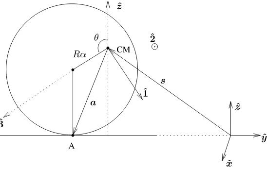
Figure 1. Model of TT.
is pointing out of the plane of the picture. The position of CM w.r.t. the inertial orthonormal reference frame (xˆ,yˆ,z) is denoted by vectorˆ sand the vector connecting CM with the pointA, of support by the horizontal plane, is denoted a = R αˆ3−zˆ
as follows from Fig. 1. The principal moments of inertia along axis (ˆ1,ˆ2,ˆ3) are denotedI1 =I2, I3 and the inertia tensor
has the form ˆI=I1✶+I3I−1I1| ˆ
3ihˆ3| , ˆI−1= I1 1
✶−I3−I1 I3 |
ˆ 3ihˆ3| .
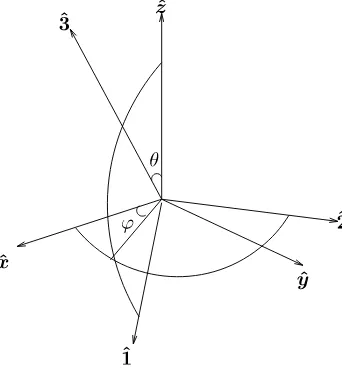
The orientation of the moving reference frame (ˆ1,ˆ2,ˆ3) w.r.t. the inertial reference frame (xˆ,yˆ,z) is described by two angles (ˆ θ, ϕ), as in Fig. 2, and the angular velocity of the moving frame can be read from Figs.1 and 2
ωref =−ϕ˙sinθˆ1+ ˙θˆ2+ ˙ϕcosθˆ3,
where dots denote time derivatives of the angles (θ, ϕ). The angular velocity of TT is then
ω=ωref+ ˙ψˆ3=−ϕ˙sinθˆ1+ ˙θˆ2+ ˙ψ+ ˙ϕcosθ
ˆ 3.
It contains an extra term ˙ψˆ3that describes rotation of TT by the angleψaround the symmetry axis ˆ3; we shall denote ω3 = ˙ψ+ ˙ϕcosθ. These definitions entail the following kinematic equations for rotation of the reference frame (ˆ1,ˆ2,ˆ3)
˙ˆ1=ωref ׈1= ˙ϕcosθˆ2−θ˙ˆ3,
˙ˆ2=ωref ׈2=−ϕ˙cosθˆ1−ϕ˙sinθˆ3,
˙ˆ3=ωref ׈3=ω×3ˆ= ˙θˆ1+ ˙ϕsinθˆ2.
The dynamics of the rolling and sliding TT is described by two ordinary differential equations (ODE’s), one for motion of CM and another one for rotation about CM
mv˙CM =FR+Ff(vA)−mgzˆ, (1a)
˙
L=a×[FR+Ff(vA)], (1b)
where vCM = ˙s, L = ˆIω is the angular momentum and vA = vCM+ω×a is the velocity of
the point of contact A. The gravity force −mgzˆ acts at the center of mass and the contact force F =FR+Ff(vA) acts at the point A. It is a sum of the friction force Ff(vA) parallel to the supporting plane and of the reaction force FR(vCM,L) that depends on the dynamical
Figure 2. Axis orientation in TT.
force we assume that it vanishes at zero sliding velocity Ff(vA=0) =0, but remarkably many qualitative aspects of the motion of TT are independent of the friction law that specifies how Ff(vA) depends on the contact velocityvA. This feature of equations (1a), (1b) is the reason why the popular toy models of TT persistently exhibit the inverting behavior for majority of supporting surfaces and for different materials that TT is made of.
In order to close the system of vector equations (1a), (1b) we need to add the equation
˙ˆ3= 1
I1
L׈3 (1c)
that follows from ˙ˆ3 =ω׈3 = ˆI−1L׈3 = I1 1
L− I3−I1 I3 L
ˆ 3ˆ
3 ׈3 = I1 1L×
ˆ
3 by the axial symmetry of TT.
In this paper we are studying only solutions that stay in the supporting plane and, there-fore, satisfy identically with respect to time t the algebraic condition zˆ[s(t) +a(t)] = 0. This condition is compatible with the structure of equations (1) if all time derivatives of ˆ
z[s(t) +a(t)] = 0 are also equal to zero. The requirement of vanishing first derivative 0 = ˆ
z ˙ s+ ˙a
= zˆ[ ˙s(t) +ω(t)×a(t)] = zvˆ A says that the contact velocity vA has to stay in the supporting plane all time and the requirement of vanishing second derivative
0 =zˆ
¨
s(t) + d
dt(ω(t)×a(t))
=zˆ
FR+Ff(vA)−mgzˆ+m d
dt(ω(t)×a(t))
=zˆ
FR−mgzˆ+m d
dt(ω(t)×a(t))
determines the vertical component of the reaction force zFˆ R = mg −mz(ω(ˆ t)×a(t)˙). The planar component of FR has to be defined as an external law of the reaction force or may be determined by some extra conditions for motions satisfying (1). For instance in the model of the rising tippe top [5, 12] there has been assumed that FR=gn(vCM,L,ˆ3)zˆis orthogonal to
the plane when Ff(vA) =−µgnvA vanishes.
In the case of pure rolling solutions it is the rolling condition that allows for determining the value of the total force F =FR (since Ff(vA = 0) =0) so that rolling without sliding takes place and FR usually is not orthogonal to the supporting plane.
we rewrite them as equations for the new unknownsvA,ˆ3and L (orω= ˆI−1L)
m ˙
vA−(ω×a˙)
=FR+Ff(vA)−mgzˆ, (2a)
˙
L=a×mgzˆ+mv˙A−m(ω×a˙)
, (2b)
˙ˆ3=ωref ׈3=ω׈3=
1
I1L×
ˆ
3. (2c)
The requirement of vanishing vA(t) = vCM(t) + [ω(t)×a(t)] = 0 entails that ˙vA = ˙vCM + (ω×a˙) = 0 vanishes as well. Then equations (2b), (2c) become an autonomous system of equations, with a polynomial vector field, for L (or ω) and ˆ3. They have solutions by the existence theorem for dynamical systems and vCM is determined from vCM = −[ω(t)×a(t)].
The condition ˙vCM=−(ω(t)×a(t)˙) automatically follows and from the first equation (2a) the
unknown total force F = FR+Ff(vA) = m
−(ω×a˙)
+mgz, needed for maintaining theˆ pure rolling motion, can be calculated. Thus we have shown.
Proposition 1. The pure rolling constraint vA = vCM +ω×a reduces equations (1) to the
closed system of equations
(ˆIω˙) =a×mgzˆ−m(ω×a˙)
, (3a)
˙ˆ3=ω׈3 (3b)
for the unknownsωandˆ3whereˆI=I1✶+I3−I1I1| ˆ
3ihˆ3| . It is consistent with equations (1)when
we assume that the total force is dynamically determined as F =FR+Ff =−m ω×a˙
+mgzˆ.
Thus the pure rolling constraint changes the model of the TT by saying that the force F applied to the body at point A is dynamically determined. This means that general rolling solutions presented here usually do not satisfy the TT model with FR = gnˆz, Ff = −µgzvA except the vertical spinning solutions and the tumbling solutions with CM fixed in space [5,12].
3
Coordinate form of the rolling TT (rTT) equations.
Integrals of motion
The autonomous system of rTT equations (3a), (3b) can be expressed in the moving reference frame ˆ1, ˆ2, ˆ3. Recall that zˆ=−sinθˆ1+ cosθˆ3, a = R(αˆ3−z) =ˆ R sinθˆ1+ (α−cosθ)ˆ3, ω=ωref+ ˙ψˆ3=−ϕ˙sinθˆ1+ ˙θˆ2+ ( ˙ψ+ ˙ϕcosθ)ˆ3=−ϕ˙sinθˆ1+ ˙θˆ2+ω3ˆ3. By substituting these
expressions into (3a) we get at ˆ1, ˆ2, ˆ3 the following system of equations for the Euler angles (θ, ϕ, ψ)
I3ω3θ˙−2I1ϕ˙θ˙cosθ−I1ϕ¨sinθ+mR2(α−cosθ) −ϕ¨sinθ(α−cosθ)
−2 ˙ϕθ˙cosθ(α−cosθ)−ω˙3sinθ−ω3θ˙cosθ
= 0, (4a)
I1θ¨−I1ϕ˙2sinθcosθ+I3ω3ϕ˙sinθ+mR2sinθ θ˙2α+ω3ϕ˙sin2θ+ ¨θsinθ
+ ˙ϕ2sin2θ(α−cosθ)
+mR2(α−cosθ) ¨θ(α−cosθ)−ϕω˙ 3sinθcosθ
−ϕ˙2sinθcosθ(α−cosθ)
=−αmgRsinθ, (4b)
I3ω˙3+mR2sinθ 2 ˙ϕθ˙cosθ(α−cosθ) + ¨ϕsinθ(α−cosθ) + ˙ω3sinθ+ω3θ˙cosθ= 0.(4c)
After resolving w.r.t. (¨θ,ϕ,¨ ω˙3) we obtain
¨
θ= sinθ
I1+mR2 (α−cosθ)2+ sin2θ
˙
ϕ2 −mR2(α−cosθ) (1−αcosθ) +I1cosθ
+ω3ϕ mR˙ 2(αcosθ−1)−I3−mR2θ˙2α−mRαg
Sinceϕandψare cyclic coordinates, that do not appear in the right hand side of equations (5), it is effectively a fourth order dynamical system for the variablesθ, ˙θ, ˙ϕ and ω3 = ˙ψ+ ˙ϕcosθ.
It admits three functionally independent integrals of motion [13]. Equation (5c) can be integrated directly to the Routh integral
D=I3ω3γ+β(α−cosθ)2+βγsin2θ
follows from equations (5b) and (5c) and the energy integral
E = 1
is a consequence of all three equations (5) as can be checked by direct differentiation w.r.t. time.
Proposition 2. The rTT equations of motion (3) admit three time independent integrals of motion
Proof . As we have seen, the coordinate form of the integrals of motion follows easily from the coordinate equations (5). It is instructive also to see how the vector form of the integrals of motion is related to the vector form of equations (3).
We see that the Jellett’s integralλ=−La is a scalar product of the angular momentumL and a vector vector a. When deriving
−λ˙ = La˙ = ˙La+La˙ = (a×F)a+L α˙ˆ3−Rz˙ˆ
=αL˙ˆ3=α 1 I1
we see that each term disappears on its own. The first term disappears because the vector a
In calculating time derivative of the energy integral we use the equality ˙ωL=ωL˙ that follows by taking the derivative of ω= ˆI−1L= I11
For rTT vA=0 and the energy is conserved since the forceF doesn’t perform any work. The Routh integral follows remarkably simple from the coordinate equation (5c) but is con-siderably more difficult to see in the vector notation. The time derivative
˙ the vector notation correspond to (4a) and (4c). We obtain two linear algebraic equations for the unknowns ω˙ˆ3
more complicated but also involves ω˙ˆ3
and ( ˙ωz) like equation (ˆ 7). From this linear system we determine ω˙ˆ3
and substitute into the ˙Dexpression. One then obtains
˙ on zˆˆ3 that vanishes identically
= 0.
In [13] and [6] a quadratic integral of motionD2is taken becauseD2 enters the expression (9) for the effective potentialV(θ;D, λ). It seems natural, however, to speak about linear integral
D = I3ω3
p
d(θ), since it is well defined due to d(θ) > 0. Any axially symmetric rolling rigid body is integrable [2,9,14] and it admits, beside energyE, a 2-parameter family of integrals of motion depending linearly on ω. These integrals are defined through transcendental functions satisfying a certain linear 2nd order ODE with variable coefficients that depend on the convex shape of the rigid body. The special feature of the rolling sphere integrals is that they are expressed explicitly through elementary functions.
4
Separation equations for rTT
Equations (5) can be considered as a fourth order system forθ, ˙θ, ˙ϕ,ω3= ˙ψ+ ˙ϕcosθsinceϕ,ψ
are cyclic variables, but it is totaly a sixth order system of equations for the Euler angles (θ, ϕ, ψ). The existence of three integrals of motion reduces the differential order by three and we obtain the system of three equations
we obtain a separable equation of the form
E =g(cosθ) ˙θ2+V(cosθ, D, λ)
least, two solutionsθ1 andθ2 and the one-dimensionalθ-motion takes place between two turning
points 0 ≤θ1, θ2 ≤ π. The motion of the symmetry axis ˆ3 on the unit sphere S2 takes place
In order to discuss the motion of the rTT we shall revoke similarities of equations (8) with the equations of the Lagrange top (LT) that follow from the Lagrangian [10]
L = 1
where the angles θ, ϕand ψ has the same meaning as for TT. The Lagrange equations of the LT admit the following three integrals of motion
L3 =I3 ψ˙+ ˙ϕcosθ
where L3,Lz and E denote the constant values of integrals. There are transparent similarities between equations (8) and (10). The Routh integral D corresponds to L3 = I3ω3, the Jellett
integral has a similar structure as Lz and in the energy E both ˙ϕ and ω3 can be eliminated
to give a one-dimensional equation for θ(t). However in the case of rTT the effective potential
V(z, D, λ) becomes a more complicated function of z than the LT effective potential VLT =
(Lz−L3cosθ)
I1 cosθ. We shall analyze the character of motions of the rTT by studying some special types of solutions that are natural counterparts of special solutions to the LT.
In the case of LT one can distinguish several types of special solutions defined by an invariant algebraic conditions for dynamical variables and/or by fixing values of integrals of motion. Their trajectories are customarily represented by a curve onS2 drawn by the symmetry axisˆ3 of LT.
a) Vertical rotations are defined by the condition θ(t)≡0 orθ(t) ≡π, so that Lz =±L3 =
and ˙ϕare also constant. They are represented by latitude circles on S2.
e) General nutational motions between two latitudes 0 ≤θ1 ≤θ2 ≤π given as solutions of
the equationE = 21I1(Lz−L3cosθ) during motion or not. There are three cases:
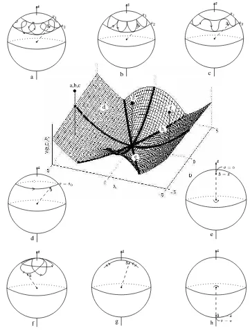
Figure 3. Illustration of the phase space picture of TT.
Due to similarity of separation equations (8) with (10) we can distinguish for rTT similar types of invariant solutions as for LT. They are easier to analyze than the general case E =
g(cosθ) ˙θ2+V(cosθ, D, λ) and they well illustrate behavior of rTT for different initial conditions.
They are again represented by curves drawn by the symmetry axis ˆ3on S2 (see Fig.3).
a) Vertical rotations defined by the condition θ(t) ≡0 or θ(t) ≡π. As for LT, the vertical rotations are represented by the north and the south pole on S2. But here for vertical motions D
λ = −1
(α∓1) γ+β(α∓1)
212 forθ= 0, π respectively.
b) Analog of planar pendulum type of solutions: D = I3ω3
p
d(θ) = 0, λ = I1ϕ˙sin2θ−
(α−cosθ)I3ω3 = 0 so that either ω3 = ˙ϕ = 0 or ω3 = 0 and θ = 0, π. The potential V(z = cosθ, D = 0, λ = 0) = mgR(1−αcosθ) is a periodic bounded function, the coefficient g(cosθ) = 12
I1 + (α−cosθ)2 + 1−cos2θ
bounded function so that rTT admits pendulum type of solutions for low values of energy as well as the “rotational” type solutions (as in the mathematical pendulum) for higher values of energy.
c) Analog of the L3 6= 0, Lz = 0 case: λ= I1ϕ˙sin2θ−(α−cosθ)I3ω3 = 0, D 6= 0 which
means that L is always in the plane orthogonal toa. Then
E =g(cosθ) ˙θ2+V(z, D, λ= 0) =g(cosθ) ˙θ2+ D is negative for z = 0, and it is not changing sign because it does not have a zero in the interval−1< z <1 for 0< α <1. The derivativep′(z) = 3 z2−1+α2 d) Analog of spherical pendulum solutions: D = ω3
p
d(θ) = 0, λ = I1ϕ˙sin2θ 6= 0 so that ω3 = 0 sinced(θ)>0 for all 0≤θ≤π. This means that during the rolling motion of rTT
it’s not performing any rotation around ˆ3-axis. Then ˙ϕ= λ
I1sin2θ and solutions will be complex and the third solution will be greater than z= 1. Because the leading term inq(z) is positive and the only real solution is greater than one, we conclude that q(z) is negative for −1< z < 1 and hence d2Vdz(z,20,λ) is positive for −1 < z <1 and
V(z= cosθ, D= 0, λ) is therefore convex. There are two types of orbits here:
(i) E =V(cosθmin, D, λ) Then the motion is along the horizontal circle atθ(t)≡θmin.
(ii) E > V(cosθmin, D, λ) Here the motion is confined between the circles 0< θ1 ≤θ2< π
which are the solutions to E =V(cosθ, λ, D= 0). Notice that ˙ϕ = λ
e) Precessional motions: ˙θ= 0 which implies thatθ(t)≡θ0, 0< θ0 < πwithω3 and ˙ϕequal
to their initial values. The motion onS2 is represented by the latitude circles (θ
0, ϕ(t)).
f) General nutational motion: The trajectory on S2 is confined between the two latitude circles (θ1, ϕ(t)) and (θ2, ϕ(t)). Where 0 ≤ θ1 ≤ θ2 ≤ π are given as solutions of the
equationE =g(cosθ) ˙θ2+V(z= cosθ, D, λ). The shape of the curve drawn byˆ3on the unit
sphere depends on whether ˙ϕ= I D 1sin2θ
λ D+
α√−cosθ d(θ)
changes sign during the motion or not.
There are three qualitatively different cases because the functionh(z) = √(α−z)
d(z) is monotone
when, −1 < z < 1. To see that h(z) is monotone observe that dhdz(z) = γ(1+β−βαz)
(d(z))32
= 0
implies z= α1 +αβ1 >1.
(i) Dλ +(α√−cosθ)
d(θ) 6= 0 for θ∈[θ1, θ2], so that ˙ϕhas the same sign during the motion, and
the trajectory (θ(t), ϕ(t)) has a wavelike form touching tangentially the two boundary latitude circlesθ1 andθ2.
(ii) Dλ + (α√−cosθ)
d(θ) = 0 forθ=θ1. In this case ˙ϕis zero at θ1, and both ˙θand ˙ϕ vanishes
at θ(t) =θ1 the motion momentarily stops, and the trajectory (θ(t), ϕ(t)) will have
cusps at the latitude θ1.
(iii) Dλ + (α√−cosθ)
d(θ) = 0 for certain θ ∈]θ1, θ2[, so that ˙ϕ changes sign during the motion,
and is positive at the latitude θ2 and negative at the latitude θ1. The trajectory
(θ(t), ϕ(t)) of theˆ3-axis on the unit sphere S2 will have a wavelike form with loops
when touching tangentially the latitude circle θ1.
All these particular types of motion are illustrated in Fig.3presenting the minimal surface of the function V(z= cosθ) in the space of parameters (D, λ, E). This surface is the lower boundary of the set of all admissible values of (D, λ, E). The values of parameters on the minimal surface corresponding to the special types of solutions are marked by distinguished black lines and the corresponding motions on the sphereS2 are illustrated by the adjacent pictures marked with the same letter. All triples of parameters (D, λ, E) describing points on the minimal surface define precessional motions θ =θ0 = const. They are denoted by the letter d. The degenerate forms
of precessional motions are the vertical rotations θ0 = 0 andθ0 = π that correspond to points
on the lines e and h. All generic points above the minimal surface of V(z) describe nutational motions denoted here by letters a, b, c. Two types of special motions corresponding to points above the minimal surface have been distinguished: the spherical pendulum type solutions that are marked by the letter f above the line D= 0 and the planar pendulum type solutions that are marked by the letter g above the point D = 0, λ = 0. The admissible set in the space of parameters (D, λ, E) represents all possible dynamical states of rTT modulo the choice of the initial angles ϕ0, ψ0 of the cyclic variables and of the initial value of the angle θ0. The time
dependence of θ(t), ϕ(t), ψ(t) is, up to these translations, fully determined by each admissible point in Fig.3.
5
Final remarks
In this paper we have discussed thoroughly the vector equations of the sliding tippe top and their reduction for pure rolling motion in the plane, the rTT equations (3a), (3b). The equations of motion (3a), (3b) admit three integrals of motion that are given here both in the vector form and also in the coordinate form, which provides the separation equations. Two integrals (D, λ), of angular momentum type, depend linearly on the momenta. Their existence can be understood as reflection of the fact that the dynamical equations (5) have two cyclic variables ϕ, ψ [14] although we are not speaking here about the Hamilton–Jacobi type separability. The third integral is the energy E that depends quadratically on momenta and gives rise to the main separation equation similarly as in the case of the Lagrange top.
According to the old result by Chaplygin [2] all axially symmetric rigid bodies rolling on the plane admit three integrals of motion – the energy and two integrals linear in momenta and are in principle separable. In general the linear integrals are however defined through two particular solutions of a second order linear differential equation with nonelementary solutions. For instance in the case of the rolling disc they are given by Legendre functions. These equations allow to formally express ˙ϕ(cosθ) and ω3(cosθ) as known functions of cosθ to be substituted
into the energy integral to give theθ-separation equation similarly as in this paper.
The special feature of the rTT equations is that the expressions for ˙ϕ(cosθ) andω3(cosθ) are
elementary functions of cosθ. When substituted explicitly into the energy integral they give an elementary expression for the effective potential V(cosθ). This simplifies analysis of equations and enables representing all possible motions in the space of parameters (D, λ, E). Only two types of stationary motion describe stable trajectories with the reaction force orthogonal to the plane. They are the stable asymptotic motions of the genuine tippe top, of vertical spinning type and the tumbling solutions when the center of mass is fixed in the space and the sphere is rolling along a circle.
The approach presented here makes it possible to perform more general study of separability and of elementary separability (when ˙ϕ(cosθ) and ω3(cosθ) can be expressed by elementary
functions) of axially symmetric rigid bodies. These questions are currently under study and the results will be presented in a subsequent paper.
Acknowledgments
The authors would like to thank referees for useful suggestions and pointing some references.
References
[1] Bou-Rabee N.M., Marsden J.E., Romero L.A., Tippe top inversion as a dissipation-induced instability,SIAM J. Appl. Dyn. Syst.3(2004), 352–377.
[2] Chaplygin S.A., On motion of heavy rigid body of revolution on horizontal plane, Proc. of the Physical Sciences, Section of the Society of Amateurs of Natural Sciences9(1897), no. 1, 10–16.
[3] Chaplygin S.A., On a ball’s rolling on a horizontal plane,Regul. Chaotic Dyn.7(2002), 131–148.
[4] Cohen R.J., The tippe top revisited,Amer. J. Phys.45(1977), 12–17.
[5] Ebenfeld S., Scheck F., A new analysis of the tippe top: asymptotic states and Liapunov stability, Ann. Physics243(1995), 195–217,chao-dyn/9501008.
[6] Gray C.G., Nickel B.G, Constants of motion for nonslipping tippe tops and other tops with rounded pegs,
Amer. J. Phys.68(1999), 821–828.
[7] Karapetyan A.V., Qualitative investigation of the dynamics of a top on a plane with friction,J. Appl. Math. Mech.55(1991), 563–565.
[8] Karapetyan A.V., On the specific character of the application of Routh’s theory to systems with differential constraints,J. Appl. Math. Mech.58(1994), 387–392.
[10] Landau L.D., Lifshitz E.M., Mechanics, Pergamon Press Ltd, Oxford, 1976.
[11] Moshchuk N.K., Qualitative analysis of the motion of a rigid body of revolution on an absolutely rough plane,J. Appl. Math. Mech.52(1988), 159–165.
[12] Rauch-Wojciechowski S., Sk¨oldstam M., Glad T., Mathematical analysis of the tippe top,Regul. Chaotic Dyn.10(2005), 333–362.
[13] Routh E.J., The advanced part of a treatise on the dynamics of a system of rigid bodies, Dover Publications, New York, 1905, 131–165.