Documenta Mathematica
Journal der
Deutschen Mathematiker-Vereinigung
Gegr¨
undet 1996
−3 −2 −1 0 1 2 3 4
−2 −1.5 −1 −0.5 0 0.5 1 1.5 2 2.5 3
X Y
Image ofS1, cf. page 518
ver¨offentlicht Forschungsarbeiten aus allen mathematischen Gebieten und wird in traditioneller Weise referiert. Es wird indiziert durch Mathematical Reviews, Science Citation Index Expanded, Zentralblatt f¨ur Mathematik.
Artikel k¨onnen als TEX-Dateien per E-Mail bei einem der Herausgeber eingereicht werden. Hinweise f¨ur die Vorbereitung der Artikel k¨onnen unter der unten angegebe-nen WWW-Adresse gefunden werden.
Documenta Mathematica, Journal der Deutschen Mathematiker-Vereinigung, publishes research manuscripts out of all mathematical fields and is refereed in the traditional manner. It is indexed in Mathematical Reviews, Science Citation Index Expanded, Zentralblatt f¨ur Mathematik.
Manuscripts should be submitted as TEX -files by e-mail to one of the editors. Hints for manuscript preparation can be found under the following web address.
http://www.math.uni-bielefeld.de/documenta
Gesch¨aftsf¨uhrende Herausgeber / Managing Editors:
Alfred K. Louis, Saarbr¨ucken [email protected]
Ulf Rehmann (techn.), Bielefeld [email protected] Peter Schneider, M¨unster [email protected]
Herausgeber / Editors:
Don Blasius, Los Angeles [email protected] Joachim Cuntz, M¨unster [email protected] Patrick Delorme, Marseille [email protected] Edward Frenkel, Berkeley [email protected] Kazuhiro Fujiwara, Nagoya [email protected] Friedrich G¨otze, Bielefeld [email protected] Ursula Hamenst¨adt, Bonn [email protected] Lars Hesselholt, Cambridge, MA (MIT) [email protected]
Max Karoubi, Paris [email protected]
Stephen Lichtenbaum Stephen [email protected]
Eckhard Meinrenken, Toronto [email protected] Alexander S. Merkurjev, Los Angeles [email protected]
Anil Nerode, Ithaca [email protected]
Thomas Peternell, Bayreuth [email protected] Eric Todd Quinto, Medford [email protected]
Takeshi Saito, Tokyo [email protected]
Stefan Schwede, Bonn [email protected]
Heinz Siedentop, M¨unchen (LMU) [email protected]
Wolfgang Soergel, Freiburg [email protected] G¨unter M. Ziegler, Berlin (TU) [email protected]
ISSN 1431-0635 (Print), ISSN 1431-0643 (Internet)
SPARC
Leading Edge
Band 12, 2007 Benoˆıt Collins, James A. Mingo,
Piotr ´Sniady, Roland Speicher Second Order Freeness and
Fluctuations of Random Matrices III.
Higher order freeness and free cumulants 1–70 Marc Levine
Motivic Tubular Neighborhoods 71–146
Andreas Langer and Thomas Zink
De Rham-Witt Cohomology and Displays 147–191 Gonc¸alo Tabuada
On the Structure of Calabi-Yau Categories
with a Cluster Tilting Subcategory 193–213 V. Gritsenko, K. Hulek and G. K. Sankaran
The Hirzebruch-Mumford Volume for
the Orthogonal Group and Applications 215–241 Jan Nekov´aˇr
On the Parity of Ranks of Selmer Groups III 243–274 Jean Fasel
The Chow-Witt ring 275–312
Christian Voigt
Equivariant Local Cyclic Homology
and the Equivariant Chern-Connes Character 313–359 Kiran S. Kedlaya
Erratum for “Slope Filtrations Revisited” 361–362 Richard Hill
Construction of Eigenvarieties in Small Cohomological Dimensions for Semi-Simple,
Simply Connected Groups 363–397
Lionel Dorat
G-Structures Entires et Modules de Wach 399–440 Alexander Schmidt
Rings of Integers of Type K(π,1) 441–471 Karim Johannes Becher, Detlev W. Hoffmann
Isotropy of Quadratic Spaces
Generic Observability of Dynamical Systems 505–520 Pierre Guillot
Geometric Methods for Cohomological Invariants 521–545 Igor Wigman
Erratum 547–548
Indranil Biswas and Johannes Huisman Rational Real Algebraic Models
of Topological Surfaces 549–567
Alexander Pushnitski and Grigori Rozenblum Eigenvalue Clusters of the Landau Hamiltonian
in the Exterior of a Compact Domain 569–586 William A. Stein
Visibility of Mordell-Weil Groups 587–606 Florian Ivorra
R´ealisationℓ-Adique
des Motifs Triangul´es G´eom´etriques I 607–671 Dimitar P. Jetchev, William A. Stein
Visibility of the Shafarevich–Tate Group
Second Order Freeness and
Fluctuations of Random Matrices III.
Higher order freeness and free cumulants
Benoˆıt Collins1, James A. Mingo2,
Piotr ´Sniady3, Roland Speicher2,4
Received: January 15, 2007
Communicated by Joachim Cuntz
Abstract. We extend the relation between random matrices and free probability theory from the level of expectations to the level of all correlation functions (which are classical cumulants of traces of products of the matrices). We introduce the notion of “higher order freeness” and develop a theory of corresponding free cumulants. We show that two independent random matrix ensembles are free of arbi-trary order if one of them is unitarily invariant. We prove R-transform formulas for second order freeness. Much of the presented theory relies on a detailed study of the properties of “partitioned permutations”.
2000 Mathematics Subject Classification: 46L54 (Primary), 15A52, 60F05
Keywords and Phrases: free cumulants, random matrices, planar di-agrams
1Research supported by JSPS and COE postdoctoral fellowships
2Research supported by Discovery Grants and a Leadership Support Initiative Award
from the Natural Sciences and Engineering Research Council of Canada
3Research supported by MNiSW (project 1 P03A 013 30), EU Research Training Network
“QP-Applications”, (HPRN-CT-2002-00279) and by European Commission Marie Curie Host Fellowship for the Transfer of Knowledge “Harmonic Analysis, Nonlinear Analysis and Prob-ability” (MTKD-CT-2004-013389)
4Research supported by a Premier’s Research Excellence Award from the Province of
1. Introduction
Random matrix models and their large dimension behavior have been an im-portant subject of study in Mathematical Physics and Statistics since Wishart and Wigner. Global fluctuations of the eigenvalues (that is, linear functionals of the eigenvalues) of random matrices have been widely investigated in the last decade; see, e.g., [Joh98, Dia03, Rad06, AZ06, MN04, M´SS07]. Roughly speaking, the trend of these investigations is that for a wide class of converging random matrix models, the non-normalized trace asymptotically behaves like a Gaussian variable whose variance only depends on macroscopic parameters such as moments. The philosophy of these results, together with the freeness results of Voiculescu served as a motivation for our series of papers on second order freeness.
One of the main achievements of the free probability theory of Voiculescu [Voi91, VDN92] was an abstract description via the notion of “freeness” of the expectation of these Gaussian variables for a large class of non-commuting tuples of random matrices.
In the previous articles of this series [MS06, M´SS07] we showed that for many in-teresting ensembles of random matrices an analogue of the results of Voiculescu for expectations holds also true on the level of variances as well; thus pointing in the direction that the structure of random matrices and the fine structure of their eigenvalues can be studied in much more detail by using the new concept of “second order freeness”. One of the main obstacles for such a detailed study was the absence of an effective machinery for doing concrete calculations in this framework. Within free probability theory of first order, such a machinery was provided by Voiculescu with the concept of the R-transform, and by Speicher with the concept of free cumulants; see, e.g., [VDN92, NSp06].
One of the main achievements of the present article is to develop a theory of second order cumulants (and show that the original definition of second order freeness from Part I of this series [MS06] is equivalent to the vanishing of mixed second order cumulants) and provide the correspondingR-transform machinery.
In Section 2 we will give a more detailed (but still quite condensed) survey of the connection between Voiculescu’s free probability theory and random matrix theory. We will there also provide the main motivation, notions and concepts for our extension of this theory to the level of fluctuations (second order), as well as the statement of our main results concerning second order cumulants andR-transforms.
the most important results (e.g. theR-transform machinery) only for first and second order, mainly because of the complexity of the underlying combinatorial objects.
The basic combinatorial notion behind the (usual) free cumulants are non-crossing partitions. Basically, passage to higher order free cumulants corre-sponds to a change to multi-annular non-crossing permutations [MN04], or more general objects which we call “partitioned permutations”. For much of the conceptual framework there is no difference between different levels of free-ness, however for many concrete questions it seems that increasing the order makes some calculations much harder. This relates to the fact thatn-th order freeness is described in terms of planar permutations which connect points onn different circles. Whereas enumeration of all non-crossing permutations in the case of one circle is quite easy, the case of two circles gets more complicated, but is still feasible; for the case of three or more circles, however, the answer does not seem to be of a nice compact form.
In the present paper we develop the notion and combinatorial machinery for freeness of all orders by a careful analysis of the main example: unitarily in-variant random matrices. We start with the calculation of mixed correlation functions for random matrices and use the structure which we observe there as a motivation for our combinatorial setup. In this way the concept of partitioned permutations and the moment–cumulant relations appear quite canonically. We want to point out that even though our notion of second and higher order freeness is modeled on the situation found for correlation functions of random matrices, this notion and theory also have some far-reaching applications. Let us mention in this respect two points.
Firstly, recently one of us [´Sni06] developed a quite general theory for fluctua-tions of characters and shapes of random Young diagrams contributing to many natural representations of symmetric groups. The results presented there are closely (though, not explicitly) related to combinatorics of higher order cumu-lants. This connection will be studied in detail in the part IV of this series where we prove that under some mild technical conditions Jucys-Murphy ele-ments, which arise naturally in the study of symmetric groups, are examples of free random variables of higher order.
In another direction, the description of subfactors in von Neumann algebras via planar algebras [Jon99] relies very much on the notions of annular non-crossing partitions and thus resembles the combinatorial objects lying at the basis of our theory of second order freeness. This indicates that our results could have some relevance for subfactors.
In Section 3 we will introduce the basic notions and relevant results on per-mutations, partitions, classical cumulants, Haar unitary random matrices, and the Weingarten function.
In Section 4 we study the correlation functions (classical cumulants of traces) of random matrix models. We will see how those are related to cumulants of entries of the matrices for unitarily invariant random matrices and we will in particular look on the correlation functions for products of two independent ensembles of random matrices, one of which is unitarily invariant. The limit of those formulas if the size N of the matrices goes to infinity will be the essence of what we are going to call “higher order freeness”. Also our main combinatorial objects, “partitioned permutations”, will arise very naturally in these calculations.
In Section 5 we will forget for a while random variables and just look on the combinatorial essence of our formulas, thus dealing with multiplicative func-tions on partitioned permutafunc-tions and their convolution. The Zeta and M¨obius functions on partitioned permutations will play an important role in these con-siderations.
In Section 6 we will derive, for the case of second order, the analogue of the R-transform formulas.
In Section 7 we will finally come back to a (non-commutative) probabilistic context, give the definition and work out the basic properties of “higher order freeness”.
In Section 8 we introduce the notion of “asymptotic higher order freeness” and show the relevance of our work for Itzykson-Zuber integrals.
In an appendix, Section 9, we provide a graphical interpretation of partitioned permutations as a special case of “surfaced permutations”.
2. Motivation and Statement of our Main Results Concerning Second Order Freeness and Cumulants
In this section we will first recall in a quite compact form the main connec-tion between Voiculescu’s free probability theory and quesconnec-tions about random matrices. Then we want to motivate our notion of second order freeness by extending these questions from the level of expectations to the level of fluc-tuations. We will recall the relevant results from the papers [MS06, M´SS07] and state the main new results of the present paper. Even though in the later parts of the paper our treatment will include freeness of arbitrarily high order, we restrict ourselves in this section mainly to the second order. The reason for this is that (apart from first order) second order freeness seems to be the most important order for applications, so that it seems worthwhile to spell out our general results for this case more explicitly. Furthermore, it is only there that we have an analogue ofR-transform formulas. We will make a few general remarks about higher order freeness at the end of this section.
about the eigenvalue distribution of the sumA+Bof the matrices? Of course, the latter is not just determined by the eigenvalues ofAand the eigenvalues of B, but also by the relation between the eigenspaces ofAand ofB. Actually, it is quite a hard problem (Horn’s conjecture) — which was only solved recently — to characterize all possible eigenvalue distributions ofA+B. However, if one is asking this question in the context ofN×N-random matrices, then in many situations the answer becomes deterministic in the limit N→ ∞.
Definition2.1. LetA= (AN)N∈Nbe a sequence ofN×N-random matrices.
We say thatAhas afirst order limit distribution if the limit of all moments
αn:= lim
N→∞E[tr(A n
N)] (n∈N)
exists and for allr >1 and all n1, . . . , nr∈N
lim
N→∞kr(tr(A n1
N),tr(A n2
N), . . . ,tr(A nr
N)) = 0,
whereE denotes the expectation, tr the normalized trace, andkr therth
clas-sical cumulant.
In this language, our question becomes: Given two random matrix ensembles ofN×N-random matrices,A= (AN)N∈NandB= (BN)N∈N, with first order
limit distribution, does also their sumC = (CN)N∈N, with CN =AN +BN,
have a first order limit distribution, and furthermore, can we calculate the limit momentsαC
n of C out of the limit moments (αAk)k≥1 ofA and the limit moments (αB
k)k≥1ofBin a deterministic way. It turns out that this is the case if the two ensembles are in generic position, and then the rule for calculating the limit moments ofCare given by Voiculescu’s concept of “freeness”. Let us recall this fundamental result of Voiculescu.
Theorem 2.2 (Voiculescu [Voi91]). Let A and B be two random matrix en-sembles of N ×N-random matrices, A= (AN)N∈N and B = (BN)N∈N, each
of them with a first order limit distribution. Assume that A and B are in-dependent (i.e., for each N ∈ N, all entries of AN are independent from all
entries of BN), and that at least one of them is unitarily invariant (i.e., for
each N, the joint distribution of the entries does not change if we conjugate the random matrix with an arbitrary unitary N×N matrix). Then A andB
are asymptotically free in the sense of the following definition.
Definition 2.3 (Voiculescu [Voi85]). Two random matrix ensembles A = (AN)N∈N and B = (BN)N∈N with limit eigenvalue distributions are
asymp-totically free if we have for all p ≥ 1 and all n(1), m(1), . . . , n(p), m(p) ≥ 1 that
lim
N→∞E
h
tr(AnN(1)−αAn(1)1)·(BNm(1)−αBm(1)1)· · ·
· · ·(An(p)
−αA
n(p)1)·(Bm(p)−αBm(p)1) i
One should realize that asymptotic freeness is actually a rule which allows to calculate all mixed moments in AandB, i.e. all expressions
lim
N→∞E[tr(A
n(1)Bm(1)An(2)Bm(2)
· · ·An(p)Bm(p))]
out of the limit moments ofAand the limit moments ofB. In particular, this means that all limit moments of A+B (which are sums of mixed moments) exist and are actually determined in terms of the limit moments ofAand the limit moments of B. The actual calculation rule is not directly clear from the above definition but a basic result of Voiculescu shows how this can be achieved by going over from the momentsαn to new quantitiesκn. In [Spe94],
the combinatorial structure behind these κn was revealed and the name “free
cumulants” was coined for them. Whereas in the later parts of this paper we will have to rely crucially on the combinatorial description and their extensions to higher orders, as well as on the definition of more general “mixed” cumulants, we will here state the results in the simplest possible form in terms of generating power series, which avoids the use of combinatorial objects.
Definition 2.4 (Voiculescu [Voi86], Speicher [Spe94]). Given the moments (αn)n≥1 of some distribution (or limit moments of some random matrix en-semble), we define the correspondingfree cumulants (κn)n≥1 by the following relation between their generating power series: If we put
M(x) := 1 +X
n≥1
αnxn and C(x) := 1 +
X
n≥1 κnxn,
then we require as a relation between these formal power series that
C(xM(x)) =M(x).
Voiculescu actually formulated the relation above in a slightly different way using the so-calledR-transformR(x), which is related to C(x) by the relation
C(x) = 1 +xR(x)
and in terms of the Cauchy transformG(x) corresponding to a measure with momentsαn, which is related toM(x) by
G(x) = M( 1
x)
x .
In these terms the equationC(xM(x)) =M(x) says that
(1) 1
G(x)+R(G(x)) =x,
i.e., thatG(x) andK(x) :=x1+R(x) are inverses of each other under compo-sition.
One should also note that the relationC(xM(x)) =M(x) determines the mo-ments uniquely in terms of the cumulants and the other way around. The relevance of the κn and the R-transform for our problem comes from the
way for calculating eigenvalue distributions of the sum of asymptotically free random matrices.
Theorem2.5 (Voiculescu [Voi86]). LetAandBbe two random matrix ensem-bles which are asymptotically free. Denote byκA
n,κBn,κAn+B the free cumulants
of A,B,A+B, respectively. Then one has for all n≥1that
κAn+B=κAn +κBn.
Alternatively,
RA+B(x) =
RA(x) +
RB(x).
This theorem is one reason for calling the κn cumulants, but there is also
another justification for this, namely they are also the limit of classical cu-mulants of the entries of our random matrix, in the case that this is unitarily invariant. This description will follow from our formulas (28) and (30). We denote the classical cumulants bykn, considered as multi-linear functionals in
narguments.
Theorem 2.6. Let A= (AN)N∈N be a unitarily invariant random matrix
en-semble ofN×N random matricesAN whose first order limit distribution exists.
Then the free cumulants of this matrix ensemble can also be expressed as the limit of special classical cumulants of the entries of the random matrices: If
AN = (a(ijN))Ni,j=1, then
κAn = lim N→∞N
n−1k
n(a(i(1)N)i(2), ai((2)N)i(3), . . . , a(iN(n)),i(1))
for any choice of distinct i(1), . . . , i(n).
2.2. Fluctuations of random matrices and asymptotic second or-der freeness. There are many more refined questions about the limiting eigenvalue distribution of random matrices. In particular, questions around fluctuations have received a lot of interest in the last decade or so. The main motivation for introducing the concept of “second order freeness” was to un-derstand the global fluctuations of the eigenvalues, which means that we look at the probabilistic behavior of traces of powers of our matrices. The limiting eigenvalue distribution, as considered in the last section, gives us the limit of the average of this traces. However, one can make more refined statements about their distributions. Consider a random matrixA= (AN)N∈N and look
on the normalized traces tr(Ak
N). Our assumption of a limit eigenvalue
dis-tribution means that the limitsαk := limN→∞E[tr(AkN)] exist. It turned out
that in many cases the fluctuation around this limit,
tr(AkN)−αk
is asymptotically Gaussian of order 1/N; i.e., the random variable
N·(tr(AkN)−αk) = Tr(ANk)−N αk= Tr(AkN −αk1)
(where Tr denotes the unnormalized trace) converges forN → ∞ to a normal variable. Actually, the whole family of centered unnormalized traces (Tr(Ak
N αk)k≥1 converges to a centered Gaussian family. (One should note that we restrict all our considerations to complex random matrices; in the case of real random matrices there are additional complications, which will be addressed in some future investigations.) Thus the main information about fluctuations of our considered ensemble is contained in the covariance matrix of the limiting Gaussian family, i.e., in the quantities
αm,n:= lim
N→∞cov(Tr(A m
N),Tr(AnN)).
Let us emphasize that the αn and the αm,n are actually limits of classical
cumulants of traces; for the first and second order, with expectation as first and variance as second cumulant, this might not be so visible, but it will become evident when we go over to higher orders. Nevertheless, theα’s will behave and will also be treated like moments; accordingly we will call theαm,n‘fluctuation
moments’. We will later define some other quantitiesκm,n, which take the role
of cumulants in this context.
This kind of convergence to a Gaussian family was formalized in [MS06] as follows. Note that convergence to Gaussian means that all higher order classical cumulants converge to zero. As before, we denote the classical cumulants by kn; so k1 is just the expectation, andk2 the covariance.
Definition2.7. LetA= (AN)N∈Nbe an ensemble ofN×N random matrices
AN. We say that it has asecond order limit distribution if for allm, n≥1 the
limits
αn:= lim
N→∞k1(tr(A n N))
and
αm,n:= lim
N→∞k2(Tr(A m
N),Tr(AnN))
exist and if
lim
N→∞kr Tr(A n(1)
N ), . . . ,Tr(A n(r)
N )
= 0
for allr≥3 and alln(1), . . . , n(r)≥1.
We can now ask the same kind of question for the limit fluctuations as for the limit moments; namely, if we have two random matrix ensemblesAandBand we know the second order limit distribution of A and the second order limit distribution ofB, does this imply that we have a second order limit distribution forA+B, and, if so, is there an effective way for calculating it. Again, we can only hope for a positive solution to this if A and B are in a kind of generic position. As it turned out, the same requirements as before are sufficient for this. The rule for calculating mixed fluctuations constitutes the essence of the definition of the concept of second order freeness.
Theorem 2.8 (Mingo, ´Sniady, Speicher [M´SS07]). Let A and B be two random matrix ensembles of N ×N-random matrices, A = (AN)N∈N and
B = (BN)N∈N, each of them having a second order limit distribution.
invariant. Then A andB are asymptotically free of second order in the sense of the following definition.
Definition 2.9 (Mingo, Speicher [MS06]). Consider two random matrix en-semblesA = (AN)N∈N andB = (BN)N∈N, each of them with a second order
if p 6= q, and otherwise (where we count modulo pfor the arguments of the indices, i.e.,n(i+p) =n(i))
Again, it is crucial to realize that this definition allows one (albeit in a com-plicated way) to express every second order mixed moment, i.e., a limit of the form
series. Let us spell out the definition here in this form. (That this is equivalent to our actual definition of the cumulants will follow from Theorem 6.3.)
Definition 2.10. Let (αn)n≥1and (αm,n)m,n≥1describe the first and second order limit moments of a random matrix ensemble. We define the corresponding
first and second order free cumulants(κn)n≥1and (κm,n)m,n≥1by the following requirement in terms of the corresponding generating power series. Put
C(x) := 1 +X
Then we require as relations between these formal power series that
(2) C(xM(x)) =M(x)
κ2,2= 18α41−36α12α2+ 6α22+ 16α1α3−4α4+ 4α21α1,1−4α1α1,2+α2,2 κ1,3= 15α41−30α21α2+ 6α22+ 12α1α3−3α4+ 6α21α1,1−3α2α1,1−3α1α1,2+α1,3
κ2,3=−72α51+ 180α31 α2−72α1α22−84α21α3+ 24α2α3+ 30α1α4−6α5
−12α31α1,1+ 6α1α2α1,1+ 12α21α1,2−3α2α1,2−2α1α1,3−3α1α2,2+α2,3 κ3,3= 300α61−900α41α2+ 576α21α22−48α32+ 432α31α3−288α1α2α3+ 18α23
−180α21α4+ 45α2α4+ 54α1α5−9α6+ 36α41α1,1−36α21α2α1,1+ 9α22α1,1
−36α31α1,2+ 18α1α2α1,2+ 12α21α1,3−6α2α1,3+ 9α21α2,2−6α1α2,3+α3,3
As in the first order case, instead of the moment power seriesM(x, y) one can consider a kind of second order Cauchy transform, defined by
G(x, y) := M( 1
x,
1
y)
xy .
If we also define a kind of second orderRtransformR(x, y) by
R(x, y) := 1
xyC(x, y), then the formula (5) takes on a particularly nice form:
(6) G(x, y) =G′(x)G′(y)nR(G(x), G(y)) + 1 (G(x)−G(y))2
o
−(x 1 −y)2. G(x) is here, as before, the first order Cauchy transform,G(x) = 1xM(1/x). The κm,n defined above deserve the name “cumulants” as they linearize the
problem of adding random matrices which are asymptotically free of second order. Namely, as will follow from our Theorem 7.15, we have the following theorem, which provides, together with (6), an effective machinery for calcu-lating the fluctuations of the sum of asymptotically free random matrices.
Theorem 2.11. Let A and B be two random matrix ensembles which are asymptotically free. Then one has for all m, n≥1 that
κAn+B=κAn +κBn and κAm,n+B =κAm,n+κBm,n.
Alternatively,
RA+B(x) =
RA(x) + RB(x)
and
RA+B(x, y) =RA(x, y) +RB(x, y).
Theorem 2.12. Let A = (AN)N∈N be a unitarily invariant random matrix
ensemble which has a second order limit distribution. Then the second order free cumulants of this matrix ensemble can also be expressed as the limit of classical cumulants of the entries of the random matrices: IfAN = (a(ijN))Ni,j=1,
then
κA
m,n= limN→∞Nm+nkm+n(a(i(1)N)i(2), ai(N(2))i(3), . . . , ai(N(m)),i(1),
aj(N(1))j(2), aj(N(2))j(3), . . . , a(jN(n)),j(1))
for any choice of distinct i(1), . . . , i(m), j(1), . . . , j(n).
This latter theorem makes it quite obvious that the second order cumulants for Gaussian as well as for Wishart matrices vanish identically, i.e., R(x, y) = 0 and thus we obtain in these cases that the second order Cauchy transform is totally determined in terms of the first order Cauchy transform (i.e., in terms of the limiting eigenvalue distribution) via
(7) G(x, y) = G′(x)G′(y) (G(x)−G(y))2 −
1 (x−y)2.
This formula for fluctuations of Wishart matrices was also derived by Bai and Silverstein in [BS04].
2.3. Higher order freeness. The idea for higher order freeness is the same as for second order one. For a random matrix ensemble A = (AN)N∈N we
define r-th order limit moments as the scaled limit of classical cumulants ofr traces of powers of our matrices,
αn1,...,nr := lim
N→∞N r−2k
r Tr(AnN(1)), . . . ,Tr(A n(r)
N )
.
in Definitions 2.3 and 2.9, respectively. For higher orders, however, we are not able to find an explicit relation of that type.
This reflects somehow the observation that our general formulas in terms of sums over partitioned permutations are the same for all orders, but that eval-uating or simplifying these sums (by doing partial summations) is beyond our abilities for orders greater than 2. Reformulating the combinatorial relation between moments and cumulants in terms of generating power series is one prominent example for this. Whereas this is quite easy for first order, the com-plexity of the arguments and the solution (given in Definition 2.10) is much higher for second order, and out of reach for higher order.
One should note that an effective (analytic or symbolic) calculation of higher order moments of a sumA+BforAandBfree of higher order relies usually on the presence of such generating power series formulas. In this sense, we have succeeded in providing an effective machinery for dealing with fluctuations (second order), but we were not able to do so for higher order.
Our results for higher orders are more of a theoretical nature. One of the main problems we have to address there is the associativity of the notion of higher order freeness. Namely, in order to be an interesting concept, our definition thatAandBare free of higher order should of course imply that any function of A is also free of higher order from any function of B. Whereas for first and second order this follows quite easily from the equivalent characterization of freeness in terms of moments as in Definitions 2.3 and 2.9, the absence of such a characterization for higher orders makes this a more complicated matter. Namely, what we have to see is that the vanishing of mixed cumulants in random variables implies also the vanishing of mixed cumulants in elements from the generated algebras. This is quite a non-trivial fact and requires a careful analysis, see section 7.
3. Preliminaries
3.1. Some general notation. For natural numbersm, n∈Nwithm < n, we denote by [m, n] the interval of natural numbers betweenmandn, i.e.,
[m, n] :={m, m+ 1, m+ 2, . . . , n−1, n}.
For a matrixA= (aij)Ni,j=1, we denote by Tr the unnormalized and by tr the normalized trace,
Tr(A) :=
N
X
i=1
aii, tr(A) := 1
NTr(A).
3.2. Permutations. We will denote the set of permutations on n elements bySn. We will quite often use the cycle notation for such permutations, i.e.,
3.2.1. Length function. For a permutationπ∈Snwe denote by #πthe number
of cycles ofπand by|π|the minimal number of transpositions needed to write πas a product of transpositions. Note that one has
|π|+ #π=n for allπ∈Sn.
3.2.2. Non-crossing permutations. Let us denote byγn∈Sn the cycle
γn = (1,2, . . . , n).
For allπ∈Sn one has that
|π|+|γnπ−1| ≤n−1.
If we have equality then we callπnon-crossing. Note that this is equivalent to #π+ #(γnπ−1) =n+ 1.
If π is non-crossing, then so are γnπ−1 and π−1γn; the latter is called the
(Kreweras) complement ofπ.
We will denote the set of non-crossing permutations in Sn by N C(n). Note
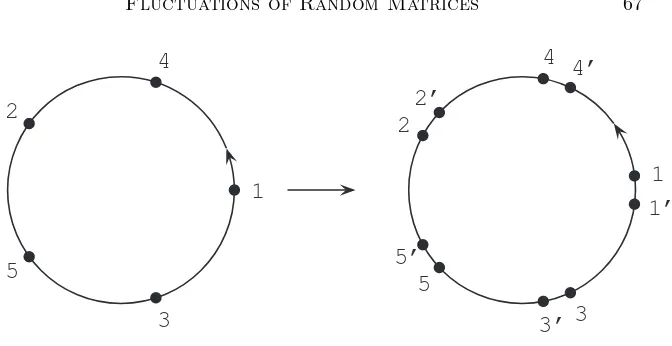
that such a non-crossing permutation can be identified with a non-crossing partition, by forgetting the order on the cycles. There is exactly one cyclic order on the blocks of a crossing partition which makes it into a non-crossing permutation.
3.2.3. Annular non-crossing permutations. Fixm, n∈ Nand denote byγm,n
the product of the two cycles
γm,n= (1,2, . . . , m)(m+ 1, m+ 2, . . . , m+n).
More generally, we shall denote byγm1,...,mk the product of the corresponding
k cycles.
We call a π ∈ Sm+n connected if the pair π and γm,n generates a transitive
subgroup inSm+n. A connected permutationπ∈Sm+n always satisfies
(8) |π|+|γm,nπ−1| ≤m+n.
Ifπis connected and if we have equality in that equation then we callπannular non-crossing. Note that if π is annular non-crossing then γm,nπ−1 is also
annular non-crossing. Again, we call the latter thecomplementofπ. Of course, all the above notations depend on the pair (m, n); if we want to emphasize this dependency we will also speak about (m, n)-connected permutations and (m, n)-annular non-crossing permutations.
We will denote the set of (m, n)-annular non-crossing permutations by SN C(m, n). A cycle of a π ∈ SN C(m, n) is called a through-cycle if it
con-tains points on both cycles. Eachπ∈SN C(m, n) is connected and must thus
have at least one through-cycle. The subset ofSN C(m, n) where all cycles are
through-cycles will be denoted bySall
N C(m, n).
partition is not one-to-one. Since we will not use the language of annular partitions in the present paper, this is of no relevance here.
Annular non-crossing permutations and partitions were introduced in [MN04]; there, many different characterizations—in particular, the one (8) above in terms of the length function—were given.
3.3. Partitions. We say that V={V1, . . . , Vk} is a partition of a set [1, n] if
the sets Vi are disjoint and non–empty and their union is equal to [1, n]. We
callV1, . . . , Vk the blocks of partitionV.
IfV ={V1, . . . , Vk} andW ={W1, . . . , Wl} are partitions of the same set, we
say that V ≤ W if for every block Vi there exists some block Wj such that
Vi ⊆ Wj. For a pair of partitions V,W we denote by V ∨ W the smallest
partition U such that V ≤ U and W ≤ U. We denote by 1n = [1, n] the
biggest partition of the set [1, n].
If π ∈ Sn is a permutation, then we can associate to π in a natural way a
partition whose blocks consist exactly of the cycles of π; we will denote this partition either by 0π ∈ P(n) or, if the context makes the meaning clear, just
byπ∈ P(n).
For a permutationπ∈Snwe say that a partitionV isπ-invariant ifπpreserves
each block ofV. This means that 0π ≤ V (which we will usually write just as
π≤ V).
IfV ={V1, . . . , Vk} is a partition of the set [1, n] and if, for 1≤i≤k, πi is a
permutation of the set Vi we denote byπ1× · · · ×πk ∈Sn the concatenation
of these permutations. We say thatπ=π1× · · · ×πk is a cycle decomposition
if additionally every factorπi is a cycle.
3.4. Classical cumulants. Given some classical probability space (Ω, P) we denote by E the expectation with respect to the corresponding probability measure,
E(a) := Z
Ω
a(ω)dP(ω)
and byL∞−(Ω, P) the algebra of random variables for which all moments exist.
Let us for the following putA:=L∞−(Ω, P).
We extend the linear functional E :A →C to a corresponding multiplicative functional on all partitions by (V ∈ P(n),a1, . . . , an ∈ A)
(9) EV[a1, . . . , an] :=
Y
V∈V
E[a1, . . . , an|V],
where we use the notation
E[a1, . . . , an|V] := E(ai1· · ·ais) for V = (i1<· · ·< is)∈ V.
Then, forV ∈ P(n), we define theclassical cumulants kV as multilinear
func-tionals onAby
(10) kV[a1, . . . , an] =
X
W∈P(n) W≤V
where M¨obP(n) denotes the M¨obius function on P(n) (see [Rot64]). The above definition is, by M¨obius inversion onP(n), equivalent to
E(a1· · ·an) =
X
π∈P(n)
kπ[a1, . . . , an].
Thekπ are also multiplicative with respect to the blocks ofV and thus
deter-mined by the values of
kn(a1, . . . , an) :=k1n[a1, . . . , an].
Note that we have in particular
k1(a) = E(a) and k2(a1, a2) = E(a1a2)−E(a1)E(a2).
An important property of classical cumulants is the following formula of Leonov and Shiryaev [LS59] for cumulants with products as arguments.
Letm, n∈Nand 1≤i(1)< i(2)<· · ·< i(m) =n. DefineU ∈ P(n) by
U = 1, . . . , i(1), i(1) + 1, . . . , i(2), . . . , i(m−1) + 1, . . . , i(m) . Consider now random variablesa1, . . . , an∈ A and define
A1: =a1· · ·ai(1) A2: =ai(1)+1· · ·ai(2)
.. .
Am: =ai(m−1)+1· · ·ai(m). Then we have
(11) km(A1, A2, . . . , Am) =
X
V∈P(n) V∨U=1n
kV[a1, . . . , an].
The sum on the right-hand side is running over those partitions ofnelements which satisfyV ∨U = 1n, which are, informally speaking, those partitions which
connect all the arguments of the cumulant km, when written in terms of the
ai.
Here is an example for this formula; fork2(a1a2, a3a4). In order to reduce the number of involved terms we will restrict to the special case where E(ai) = 0
(and thus also k1(ai) = 0) for all i = 1,2,3,4. There are three partitions
π∈ P(4) without singletons which satisfy
π∨ {(1,2),(3,4)}= 14,
and thus formula (11) gives in this case
k2(a1a2, a3a4) =k4(a1, a2, a3, a4)
+k2(a1, a4)k2(a2, a3) +k2(a1, a3)k2(a2, a4).
As a consequence of (11) one has the following important corollary: If
{a1, . . . , an} and{b1, . . . , bn} are independent then
(12) kW[a1b1, . . . , anbn] =
X
V,V′ ∈P(n) V∨V′=W
kV[a1, . . . , an]·kV′[b1, . . . , bn].
3.5. Haar distributed unitary random matrices and the Wein-garten function. In the following we will be interested in the asymptotics of special matrix integrals over the group U(N) of unitary N ×N-matrices. We always equip the compact groupU(N) with its Haar probability measure. A random matrix whose distribution is this measure will be called aHaar dis-tributed unitary random matrix. Thus the expectation E over this ensemble is given by integrating with respect to the Haar measure.
The expectation of products of entries of Haar distributed unitary random matrices can be described in terms of a special function on the permutation group. Since such considerations go back to Weingarten [Wei78], Collins [Col03] calls this function the Weingarten function and denotes it by Wg. We will follow his notation. In the following we just recall the relevant information about this Weingarten function, for more details we refer to [Col03, C´S06]. We use the following definition of the Weingarten function. For π∈ Sn and
N ≥nwe put
Wg(N, π) = E[u11· · ·unnu1π(1)· · ·unπ(n)],
where U = (uij)Ni,j=1 is an N ×N Haar distributed unitary random matrix. Sometimes we will suppress the dependency onN and just write Wg(π). This Wg(N, π) depends only on the conjugacy class ofπ. General matrix integrals over the unitary group can be calculated as follows:
(13) E[ui′
1j′1· · ·ui′nj′nui1j1· · ·uinjn]
= X
α,β∈Sn
δi1i′α(1)· · ·δini′α(n)δj1j′β(1)· · ·δjnjβ′(n)Wg(βα
−1).
This formula for the calculation of moments of the entries of a Haar unitary random matrix bears some resemblance to the Wick formula for the joint mo-ments of the entries of Gaussian random matrices; thus we will call (13) the
Wick formula for Haar unitary matrices.
3.6. Cumulants of the Weingarten function. We will also need some (classical) relative cumulants of the Weingarten function, which were intro-duced in [Col03, §2.3]. As before, let M¨obP(n) be the M¨obius function on the partially ordered set of partitions of [1, n] ordered by inclusion.
Let us first extend the Weingarten function by multiplicative extension, for
V ≥π, by
Wg(V, π) := Y
V∈V
Wg(π|V),
where π|V denotes the restriction ofπ to the blockV ∈ V (which is invariant
under πsinceπ≤ V).
The relative cumulant of the Weingarten function is now, for σ ≤ V ≤ W, defined by
(14) CV,W(σ) =
X
U∈P(n) V≤U≤W
M¨ob(U,W)·Wg(U, σ).
Note that, by M¨obius inversion, this is, for anyσ≤ V ≤ W, equivalent to
(15) Wg(W, σ) = X
U∈P(n) V≤U≤W
CV,U(σ).
In [Col03, Cor. 2.9] it was shown that the order ofCV,W(σ) is at most
(16) N−2n+#σ+2#W−2#V.
4. Correlation functions for random matrices
4.1. Correlation functions and partitioned permutations. Let us consider N×N-random matrices B1, . . . , Bn : Ω→MN(C). The main
infor-mation we are interested in are the “correlation functions”ϕnof these matrices,
given by classical cumulants of their traces, i.e.,
ϕn(B1, . . . , Bn) :=kn(Tr(B1), . . . ,Tr(Bn)).
Even though these correlation functions are cumulants, it is more adequate to consider them as a kind of moments for our random matrices. Thus, we will also call them sometimescorrelation moments.
We will also need to consider traces of products which are best encoded via permutations. Thus, for π ∈ Sn, ϕ(π)[B1, . . . , Bn] shall mean that we take
cumulants of traces of products along the cycles of π. For an n-tuple B = (B1, . . . , Bn) of random matrices and a cyclec= (i1, i2, . . . , ik) withk≤nwe
denote
B|c :=Bi1Bi2· · ·Bik.
(We do not distinguish between products which differ by a cyclic rotation of the factors; however, in order to make this definition well-defined we could normalize our cyclec= (i1, i2, . . . , ik) by the requirement thati1is the smallest among the appearing numbers.) For any π ∈ S(n) and any n-tuple B = (B1, . . . , Bn) of random matrices we put
whereπconsists of the cyclesc1, . . . , cr.
Example:
ϕ((1,3)(2,5,4))[B1, B2, B3, B4, B5] =ϕ2(B1B3, B2B5B4)
=k2(Tr(B1B3),Tr(B2B5B4)) Furthermore, we also need to consider more general products of such ϕ(π)’s. In order to index such products we will use pairs (V, π) whereπis, as above, an element in Sn, andV ∈ P(n) is a partition which is compatible with the
cycle structure ofπ, i.e., each block of V is fixed underπ, or to put it another way, V ≥π. In the latter inequality we use the convention that we identify a permutation with the partition corresponding to its cycles if this identification is obvious from the structure of the formula; we will write this partition 0π or
just 0 if no confusion will result.
Notation4.1. Apartitioned permutation is a pair (V, π) consisting ofπ∈Sn
andV ∈ P(n) withV ≥π. We will denote the set of partitioned permutations ofnelements byPS(n). We will also put
PS:= [
n∈N PS(n).
For such a (V, π)∈ PS we denote finally ϕ(V, π)[B1, . . . , Bn] :=
Y
V∈V
ϕ(π|V)[B1, . . . , Bn|V].
Example:
ϕ {1,3,4}{2},(1,3)(2)(4)[B1, B2, B3, B4]
=ϕ2(B1B3, B4)·ϕ1(B2)
=k2(Tr(B1B3),Tr(B4))·k1(Tr(B2)) Let us denote by Trσ as usual a product of traces along the cycles ofσ. Then
we have the relation
E{Trσ[A1, . . . , An]}=
X
W∈P(n) W≥σ
ϕ(W, σ)[A1, . . . , An].
By using the formula (11) of Leonov and Shiryaev one sees that in terms of the entries of our matrices Bk= (b(ijk))Ni,j=1 ourϕ(U, γ) can also be written as
(17) ϕ(U, γ)[B1, . . . , Bn] =
X
V≤U V∨γ=U
N
X
i(1),...,i(n)=1
kV[b(1)i(1)i(γ(1)), . . . , b (n)
i(n)i(γ(n))].
Definition4.2. Random matricesA1, . . . , Anare calledunitarily invariant if
the joint distribution of all their entries does not change by global conjugation with any unitary matrix, i.e., if, for any unitary matrixU, the matrix-valued random variablesA1, . . . , An : Ω→MN(C) have the same joint distribution as
the matrix-valued random variablesU A1U∗, . . . , U AnU∗: Ω→MN(C).
Let A1, . . . , An be unitarily invariant random matrices. We will now try
ex-pressing the microscopic quantities “cumulants of entries of the Ai” in terms
of the macroscopic quantities “cumulants of traces of products of theAi”.
In order to make this connection we have to use the unitary invariance of our ensemble. By definition, this means thatA1, . . . , An has the same distribution
as ˜A1, . . . ,A˜n where ˜Ai := U AiU∗. Since this holds for any unitary U, the
same is true after averaging over such U, i.e., we can take in the definition of the ˜Ai the U as Haar distributed unitary random matrices, independent
from A1, . . . , An. This reduces calculations for unitarily invariant ensembles
We can extend the above to products of expectations by
whereG(V, π) is given by multiplicative extension:
G(V, π)[A1, . . . , An] : =
Now we can look on the cumulants of the entries of our unitarily invariant matricesAi; they are given by
kVa(1)p1r1, . . . , a we can write this also as
Remark 4.3. 1) Note that although the quantityκis defined by (20) in terms of the macroscopic moments of theAi, they have also a very concrete meaning
in terms of cumulants of entries of the Ai. Namely, if we choose π ∈ Sn
and distinct 1≤i(1), . . . , i(n)≤N then equation (21) becomes, when we set
V = 1n,
(23) κ(1n, π)[A1, . . . , An] =kn a(1)i(1)i(π(1)), . . . , a(in(n))i(π(n))
as the the only term in the sum that survives is the one forπ.
2) Equation (22) should be considered as a kind of moment-cumulant formula in our context, thus it should contain all information for defining the “cumulants” κ in terms of the moments ϕ. Actually, we can solve this linear system of equations forκin terms ofϕ, by using equation (20) to defineκand equation (19) for G.
κ(V, π)[A1, . . . , An]
= X
U∈P(n) V≥U≥π
M¨obP(n)(U,V)· X
(W,σ)∈PS(n) W≤U
Wg(U, σπ−1)
·ϕ(W, σ)[A1, . . . , An]
= X
(W,σ)∈PS(n)
ϕ(W, σ)[A1, . . . , An]·
X
U∈P(n) V≥U≥π∨W
M¨obP(n)(U,V)·Wg(U, σπ−1).
Thus, by using the relative cumulants of the Weingarten function from (14), we get finally
(24) κ(V, π)[A1, . . . , An] =
X
(W,σ)∈PS(n)
W≤V
ϕ(W, σ)[A1, . . . , An]·Cπ∨W,V(σπ−1).
3) One should also note that we have defined the Weingarten function only for N ≥n; thus in the above formulas we should always consider sufficiently largeN. This is consistent with the observation that the system of equations (22) might not be invertible forN too small; the matrix N#(σπ−1)
σ,π∈Sn is
invertible for N ≥n, however, in general not for all N < n (e.g, clearly not for N = 1). One can make sense of some formulas involving the Weingarten function also forN < n(see [C´S06]). However, since we are mainly interested in the asymptotic behavior of our formulas forN → ∞, we will not elaborate on this.
4.3. Product of two independent ensembles. Let us now calculate the correlation functions for a product of two independent ensembles A1, . . . , An
and B1, . . . , Bn of random matrices, where we assume that one of them, let’s
say the Bi’s, is unitarily invariant. We have, by using (17) and the special
ϕ(U, γ)[A1B1, . . . , AnBn]
In order to evaluate the second factor we note first that, under the assumption π≤ V, the conditionV′∨ V ∨γ=U is equivalent toV′∨ V ∨π−1γ=U. Next,
Let us summarize the result of our calculations in the following theorem. In order to indicate that our main formulas are valid for any fixed N, we will decorate the relevant quantities with a superscript (N). Note that up to now we have not made any asymptotic consideration.
Theorem 4.4. Let MN := MN ⊗L∞(Ω) be an ensemble of N ×N-random
MN)
(25) ϕ(nN)(D1, . . . , Dn) :=kn(Tr(D1), . . . ,Tr(Dn))
and corresponding “cumulant functions”κ(N) (for n
≤N) by
(26)
κ(N)(V, π)[D1, . . . , Dn] =
X
W∈P(n), σ∈Sn
W≤V
ϕ(N)(W, σ)[D1, . . . , Dn]·Cπ(N∨W) ,V(σπ− 1),
or equivalently by the implicit system of equations
ϕ(N)(U, γ)[D1, . . . , Dn] =
X
V,π
κ(N)(V, π)[D1, . . . , Dn]·N#(γπ
−1) , (27)
where the sum is over all V ∈ P(n)allπ∈Sn such thatπ≤ VandV ∨γπ−1= U.
1) LetAN be an algebra of unitarily invariant random matrices inMN. Then
we have for all n≤N, all distinct i(1), . . . , i(n), all Ak = a(ijk)
N
i,j=1 ∈ AN,
and all π∈Sn that
(28) κ(N)(1n, π)[A1, . . . , An] =kn a(1)i(1)i(π(1)), . . . , a(in(n))i(π(n)).
2) Assume that we have two subalgebras AN andBN of MN such that ⋄ AN is a unitarily invariant ensemble,
⋄ AN andBN are independent.
Then we have for all n ∈ N with n ≤ N and all A1, . . . , An ∈ AN and
B1, . . . , Bn∈ BN:
(29) ϕ(N)(U, γ)[A1B1, . . . , AnBn]
= X
V,π,W,σ
κ(N)(V, π)[A1, . . . , An]·ϕ(N)(W, σ)[B1, . . . , Bn],
where the sum is over all V,W ∈ P(n) and all π, σ ∈ Sn such that π ≤ V,
σ≤ W,V ∨ W=U, andγ=πσ.
4.4. LargeN asymptotics for moments and cumulants. Our main in-terest in this paper will be the largeN limit of formula (29). This structure in leading order between independent ensembles of random matrices which are randomly rotated against each other will be captured in our abstract notion of higher order freeness.
Definition 4.5. Let, for each N ∈ N, B(1N), . . . , B (N)
r ⊂ MN ⊗L∞−(Ω) be
N ×N-random matrices. Suppose that the leading term of the correlation moments of B1(N), . . . , B
(N)
r are of order 2−n, i.e., that for alln∈Nand all
polynomialsp1, . . . , ptin rnon-commuting variables the limits
lim
N→∞ϕ (N)
n (p1(B1(N), . . . , Br(N)), . . . , pt(B1(N), . . . , Br(N)))·Nn−2
exist. Then we will say that {B1(N), . . . , Br(N)} has limit distributions of all
orders. LetB be the free algebra generated by generatorsb1, . . . , br. Then we
define thelimit correlation functionsofBby ϕn(p1(b1, . . . , br), . . . , pt(b1, . . . , br))
= lim
N→∞ϕ (N)
n (p1(B1(N), . . . , B(rN)), . . . , pt(B1(N), . . . , Br(N)))·Nn−2
Note that this assumption implies that the leading term for the quantities ϕ(N)(
V, π) is of order 2#(V)−#(π). Indeed, if V has k blocks and the ith
block of V contains ri cycles of πthen ϕ(N)(V, π) =ϕr1· · ·ϕrk and eachϕri
has order 2−ri. Then the order of ϕ(N)(V, π) is (2−r1) +· · ·+ (2−rk) =
2k−(r1+· · ·+rk) = 2 #(V)−#(π). Thus
ϕ(V, π)(p1(b1, . . . , br), . . . , pt(b1, . . . , br))
= lim
N→∞ϕ (N)(
V, π)(p1(B(1N), . . . , B(rN)), . . . , pt(B1(N), . . . , Br(N))) ·N−2#(V)+#(π)
From formula (27) one can deduce that the leading order ofκ(N)(
V, π) is given by the term (U, γ) = (V, π) and thus must be of order
N−n+2#V−#π.
(Indeed, this also follows from equation (24) and the leading order of the relative cumulant of the Weingarten function given in equation (16).)
Thus we can define the limiting cumulant functions to be the limit of the leading order of the cumulants by the equation
(30) κ(V, π)[b1, . . . , bn] := lim N→∞N
n−2#V+#π
·κ(N)(V, π)[B1(N), . . . , B(nN)]
When (V, π) = (1n, γn) andB1=B2=· · ·=Bn=B equation (28) becomes
κ(N)(1n, γn)[B, . . . , B] =kn bi((1)N)i(2), . . . , bi((Nn))i(1))
Thus to prove Theorem 2.6 we must show that κ(N)(1
n, γn)[B, . . . , B]·Nn−1
converges toκb
n thenthfree cumulant of the limiting eigenvalue distribution of
B(N).
When (V, π) = (1m+n, γm,n) equation (28) becomes
Thus to prove Theorem 2.12 we must show that κ(N)(1
m+n, γm,n)[B, . . . , B]·
Nm+n converges to κb
m,n the (m, n)th free cumulant of second order of the
limiting second order distribution ofB(N).
4.5. Length functions. We want to understand the asymptotic behavior of formula (29). The leading order inN of the right hand side is given by
−n+ 2#V −#π+ 2#W −#σ=n+ (|π| −2|V|) + (|σ| −2|W|), whereas the leading order of the left hand side is given by
2#U −#γ= 2#(V ∨ W)−#(σπ) =n+ (|πσ| −2|V ∨ W|).
This suggests the introducing of the following “length functions” for permuta-tions, partipermuta-tions, and partitioned permutations.
Notation 4.6.
(1) ForV ∈ P(n) andπ∈Sn we put |V|:=n−#V
|π|:=n−#π. (2) For any (V, π)∈ PS(n) we put
|(V, π)|:= 2|V| − |π|=n−(2#V −#π).
Let us first observe that these quantities behave actually like a length. It is clear from the definition that they are always non-negative; that they also obey a triangle inequality is the content of the next lemma.
Lemma 4.7.
(1) For all π, σ∈Sn we have
|πσ| ≤ |π|+|σ|. (2) For all V,W ∈ P(n)we have
|V ∨ W| ≤ |V|+|W|.
(3) For all partitioned permutations(V, π),(W, σ)∈ PS(n)we have
|(V ∨ W, πσ)| ≤ |(V, π)|+|(W, σ)|.
Proof. (1) This is well-known, since|π|is the minimal number of factors needed to writeπas a product of transpositions.
(2) Each blockB of W can glue at most #B−1 many blocks ofV together, i.e.,Wcan glue at mostn−#Wmany blocks ofVtogether, thus the difference between|V|and|V ∨ W|cannot exceedn−#W and hence
#V −#(V ∨ W)≤n−#W. This is equivalent to our assertion.
(3) We prove this, for fixedπandσby induction over|V|+|W|. The smallest possible value of the latter appears for |V| =|π| and |W|= |σ| (i.e., V = 0π
andW = 0σ). But then we have (sinceV ∨ W ≥πσ)
which is exactly our assertion for this case. For the induction step, on the other side, one only has to observe that if one increases |V| (or |W|) by one then|V ∨ W| can also increase by at most 1.
Remark 4.8. 1) Note that the triangle inequality for partitioned permutations together with (29) implies the following. Given random matricesA= (AN)N∈N
andB= (BN)N∈Nwhich have limit distributions of all orders. IfAandBare
independent and at least one of them is unitarily invariant, thenC= (CN)N∈N
withCN :=ANBN also has limit distributions of all orders.
2) Since we know that Gaussian and Wishart random matrices have limit dis-tributions of all orders (see e.g. [MS06, Thm. 3.1 and Thm. 3.5]), and since they are unitarily invariant, it follows by induction from the previous part that any polynomial in independent Gaussian and Wishart matrices has limit distributions of all orders.
4.6. Multiplication of partitioned permutations. Suppose {B1(N), . . . , Bn(N)} has limit distributions of all orders. Then the left hand side of
equation (27) has orderN2#(U)−#(γ)and the right hand side of equation (27) has orderN−n+2#(V)−#(π)+|γπ−1|. Thus the only terms of the right hand side
that have orderN2#(U)−#(γ)are those for which
2#(U)−#(γ) =−n+ 2#(V)−#(π) +|γπ−1|
i.e. for which |(U, γ)|=|(V, π)|+|γπ−1
|. Hence
ϕ(N)(U, γ)[B1(N), . . . , B(nN)]
= X
(V,π)∈PS(n) V∨γπ−1=U |(U,γ)|=|(V,π)|+|γπ−1|
κ(N)(
V, π)[B(1N), . . . , B(N)
n ]·N|γπ
−1 |
+O(N2#(U)−#(γ)−2)
Thus after taking limits we have
(31) ϕ(U, γ)[b1, . . . , bn] =
X
(V,π)∈PS(n)
κ(V, π)[b1, . . . , bn]
where the sum is over all (V, π) inPS(n) such thatV ∨γπ−1=
U and|(U, γ)|=
|(V, π)|+|γπ−1
|.
A similar analysis of equation (29) gives that for independent{A(1N), . . . , A(nN)}
and{B1(N), . . . , Bn(N)}with theA(iN)’s unitarily invariant and both having limit
ϕ(N)(U, γ)[A(1N)B (N)
1 , . . . , A(nN)Bn(N)]
= X
(V,π),(W,σ)∈PS(n) V∨W=U, πσ=γ
|(V,π)|+|(W,σ)|=|(V∨W,πσ)|
κ(N)(V, π)[A(1N), . . . , An(N)]·ϕ(N)(W, σ)[B
(N)
1 , . . . , Bn(N)]
+O(N2#(U)−#(γ)−2) and again after taking limits
(32) ϕ(U, γ)[a1b1, . . . , anbn]
= X
(V,π),(W,σ)∈PS(n)
κ(V, π)[a1, . . . , an]·ϕ(W, σ)[b1, . . . , bn]
where the sum is over all (V, π),(W, σ)∈ PS(n) such that
⋄ V ∨ W=U ⋄ πσ=γ
⋄ |(V, π)|+|(W, σ)|=|(U, γ)|
In order to write this in a more compact form it is convenient to define a multiplication for partitioned permutations (inCPS(n)) as follows.
Definition4.9. For (V, π),(W, σ)∈ PS(n) we define their product as follows. (33) (V, π)·(W, σ) :=
= (
(V ∨ W, πσ) if|(V, π)|+|(W, σ)|=|(V ∨ W, πσ)|,
0 otherwise.
Proposition4.10. The multiplication defined in Definition 4.9 is associative. Proof. We have to check that
(34) (V, π)·(W, σ)·(U, τ) = (V, π)· (W, σ)·(U, τ).
Since both sides are equal to (V ∨ W ∨ U, πστ) in case they do not vanish, we have to see that the conditions for non-vanishing are for both sides the same. The conditions for the left hand side are
|(V, π)|+|(W, σ)|=|(V ∨ W, πσ)|
and
|(V ∨ W, πσ)|+|(U, τ)|=|(V ∨ W ∨ U, πστ)|. These imply
|(V, π)|+|(W, σ)|+|(U, τ)|=|(U ∨ W ∨ U, πστ)|
≤ |(V, π)|+|(W ∨ U, στ)|, However, the triangle inequality
yields that we have actually equality in the above inequality, thus leading to
|(W, σ)|+|(U, τ)|=|(W ∨ U, στ)| and
|(V, π)|+|(W ∨ U, στ)|=|(V ∨ W ∨ U, πστ)|.
These are exactly the two conditions for the vanishing of the right hand side of (34). The other direction goes analogously.
Now we can write formulas (31) and (32) in convolution form
(35) ϕ(U, γ)[b1, . . . , bn] =
X
(V,π)∈PS(n) (V,π)·(0,γπ−1 )=(U,γ)
κ(V, π)[b1, . . . , bn]
and
(36) ϕ(U, γ)[a1b1, . . . , anbn]
= X
(V,π),(W,σ)∈PS(n) (V,π)·(W,σ)=(U,γ)
κ(V, π)[a1, . . . , an]·ϕ(W, σ)[b1, . . . , bn].
Note that both ϕ(V, π) and κ(V, π) are multiplicative in the sense that they factor according to the decomposition ofV into blocks.
The philosophy for our definition of higher order freeness will be that equation (35) is the analogue of the moment-cumulant formula and shall be used to define the quantitiesκ, which will thus take on the role of cumulants in our theory – whereas theϕ are the moments (see Definition 7.4). We shall define higher order freeness by requiring the vanishing of mixed cumulants, see Definition 7.6. On the other hand, equation (36) would be another way of expressing the fact that the a’s are free from the b’s. Of course, we will have to prove that those two possibilities are actually equivalent (see Theorem 7.9).
5. Multiplicative functions on partitioned permutations and their convolution
5.1. Convolution of multiplicative functions. Formulas (35) and (36) above are a generalization of the formulas describing first order freeness in terms of cumulants and convolution of multiplicative functions on non-crossing partitions. Since the dependence on the random matrices is irrelevant for this structure we will free ourselves in this section from the random matrices and look on the combinatorial heart of the observed formulas. In Section 7, we will return to the more general situation involving multiplicative functions which depend also on random matrices or more generally elements from an algebra.
Definition 5.1.
(1) We denote byPS the set of partitioned permutations on an arbitrary number of elements, i.e.,
PS= [
(2) For two functions
f, g:PS →C
we define their convolution
f∗g:PS →C
by
(f ∗g)(U, γ) := X (V,π),(W,σ)∈PS(n)
(V,π)·(W,σ)=(U,γ)
f(V, π)g(W, σ)
for any (U, γ)∈ PS(n).
Definition 5.2. A function f : PS → C is called multiplicative if f(1n, π)
depends only on the conjugacy class ofπand we have f(V, π) = Y
V∈V
f(1V, π|V).
Our main interest will be in multiplicative functions. It is easy to see that the convolution of two multiplicative functions is again multiplicative. It is clear that a multiplicative function is determined by the values of f(1n, π) for all
n∈Nand allπ∈Sn.
An important example of a multiplicative function is theδ-function presented below.
Notation5.3. Theδ-function onPSis the multiplicative function determined by
δ(1n, π) =
(
1 ifn= 1, 0 otherwise.
Thus for (U, π)∈ PS(n) δ(U, π) =
(
1 if (U, π) = 0n,(1)(2). . .(n)for somen,
0 otherwise.
Proposition 5.4. The convolution of multiplicative functions onPS is com-mutative and δis the unit element.
Proof. It is clear thatδis the unit element. For commutativity, we note that for multiplicative functions we have
f(V, π) =f(V, π−1), and thus
(g∗f)(U, γ) = (g∗f)(U, γ−1) = X (V,π),(W,σ)∈PS(n) (V,π)·(W,σ)=(U,γ−1 )
g(V, π)f(W, σ).
Since the condition (V, π)·(W, σ) = (U, γ−1) is equivalent to the condition (W, σ−1)·(V, π−1) = (U, γ) we can continue with
(g∗f)(U, γ) = X (V,π),(W,σ)∈PS(n) (W,σ−1 )·(V,π−1 )=(U,γ)
5.2. Factorizations. Let us now try to characterize the non-trivial factor-izations (U, γ) = (V, π)·(W, σ) appearing in the definition of our convolution. Let us first observe some simple general inequalities.
Lemma 5.5.
(1) For permutationsπ, σ∈S(n)we have
|π|+|σ|+|πσ| ≥2|π∨σ|. (2) For partitionsV2≤ V1 andW2≤ W1 we have
|W1|+|V1|+|V2∨ W2| ≥ |V1∨ W1|+|W2|+|V2|
and
|V1∨ W2|+|V2∨ W1| ≥ |V1∨ W1|+|V2∨ W2|.
Proof. (1) By the triangle inequality for partitioned permutations we have
|(0π∨0σ, πσ)| ≤ |(0π, π)|+|(0σ, σ)|,
i.e.,
(37) 2|π∨σ| − |πσ| ≤ |π|+|σ|.
(2) Consider first the special case W1=W2=W. Then we clearly have #(V2∨ W)−#(V1∨ W)≤#V2−#V1,
which leads to
|V1∨ W| − |V2∨ W| ≤ |V1| − |V2|. From this the general case follows by
|V1∨ W1| − |V2∨ W2|=|V1∨ W1| − |V1∨ W2|+|V1∨ W2| − |V2∨ W2|
≤ |W1| − |W2|+|V1| − |V2|. The second inequality follows from this as follows:
|V1∨ W1| − |V1∨ W2|=|V1∨(V2∨ W1)| − |V1∨(V2∨ W2)|
≤ |V2∨ W1| − |V2∨ W2|.
Theorem 5.6. For(V, π),(W, σ)∈ PS(n)the equation
(V, π)·(W, σ) = (V ∨ W, πσ)
is equivalent to the conjunction of the following four conditions:
|π|+|σ|+|πσ|= 2|π∨σ|,
|V|+|π∨σ|=|π|+|V ∨σ|,
|W|+|π∨σ|=|σ|+|π∨ W|,
Proof. Adding the four inequalities given by Lemma 5.5
|π|+|σ|+|πσ| ≥2|π∨σ|, 2|V|+ 2|π∨σ| ≥2|π|+ 2|V ∨σ|, 2|W|+ 2|π∨σ| ≥2|σ|+ 2|π∨ W|, 2|V ∨σ|+ 2|π∨ W| ≥2|V ∨ W|+ 2|π∨σ| gives
2|V| − |π|+ 2|W| − |σ| ≥2|V ∨ W| − |πσ|, i.e.,
|(V, π)|+|(W, σ)| ≥ |(V ∨ W, πσ).
Since (V, π)·(W, σ) = (V ∨ W, πσ) means that we require equality in the last inequality, this is equivalent to having equality in all the four inequalities.
The conditions describing our factorizations have a quite geometrical meaning. Let us elaborate on this in the following.
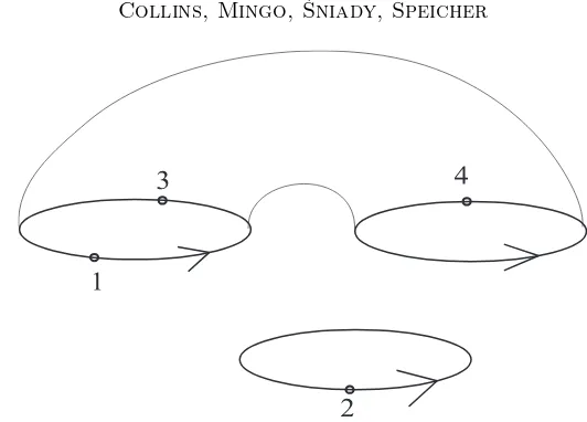
Definition 5.7. Letγ∈S(n) be a fixed permutation. (1) A permutationπ∈S(n) is calledγ-planar if
|π|+|π−1γ
|+|γ|= 2|π∨γ|.
(2) A partitioned permutation (V, π)∈ PS(n) is calledγ-minimal if
|V ∨γ| − |π∨γ|=|V| − |π|.
Remark 5.8. i) It is easy to check (for example, by calculating the Euler char-acteristic) that γ-planarity of π corresponds indeed to a planar diagram, i.e. one can draw a planar graph representing permutationsγ and πwithout any crossings. The most important cases are when γ consists of a single cycle [Bia97] and whenγconsists of two cycles [MN04].
ii) The notion ofγ-minimality of (V, π) means thatV connects only blocks of πwhich are not already connected byγ.
iii) If (V, π) satisfies both (1) and (2) of Definition 5.7 then (V, π)(0, π−1γ) = (1, γ), by Theorem 5.6.
Corollary 5.9. Assume that we have the equation
(U, γ) = (V, π)·(W, σ).
Then π andσmust beγ-planar and(V, π)and(W, σ) must beγ-minimal.
5.3. Factorizations of disc and tunnel permutations.
Notation 5.10. i ) We call (V, π)∈ PSn a disc permutation if V = 0π; the
latter is equivalent to the condition |V| =|σ|. Forπ ∈ Sn, by (0, π) we will
always mean the disc permutation
(0, π) := (0π, π)∈ PS(n).
A motivation for those names comes from the identification between partitioned permutations and so-called surfaced permutations; see the Appendix for more information on this.
Our goal is now to understand more explicitly the factorizations of disc and tunnel permutations. (It will turn out that those are the relevant ones for first and second order freeness). For this, note that we can rewrite the crucial condition for our product of partitioned permutations,
2|V| − |π|+ 2|W| − |σ|= 2|V ∨ W| − |πσ|, in the form
|V| − |π|+ |W| − |σ|+ |V|+|W| − |V ∨ W|= |V ∨ W| − |πσ|. Since all terms in brackets are non-negative integers this formula can be used to obtain explicit solutions to our factorization problem for small values of the right hand side. Essentially, this tells us that factorizations of a disc per-mutation can only be of the form disc×disc; and factorizations of a tunnel permutation can only be of the form disc×disc, disc×tunnel, and tunnel×disc. Of course, one can generalize the following arguments to higher order type per-mutations, however, the number of possibilities grows quite quickly.
Proposition5.11.
(1) The solutions to the equation
(1n, γn) = (0, γn) = (V, π)·(W, σ)
are exactly of the form
(1n, γn) = (0, π)·(0, π−1γn),
for someπ∈N C(n).
(2) The solutions to the equation
(1m+n, γm,n) = (V, π)·(W, σ)
are exactly of the following three forms:
(a)
(1m+n, γm,n) = (0, π)·(0, π−1γm,n),
whereπ∈SN C(m, n);
(b)
(1m+n, γm,n) = (0, π)·(W, π−1γm,n),
whereπ∈N C(m)×N C(n),|W|=|π−1γm,n|+1, andWconnects
a cycle ofπ−1γm,n inN C(m)with a cycle inN C(n);
(c)
(1m+n, γm,n) = (V, π)·(0, π−1γm,n),
whereπ∈N C(m)×N C(n),|V|=|π|+ 1, and|W|=|π−1γ
m,n|+