Jurnal Ekonomi dan Studi Pembangunan Volume 8, Nomor 2, Oktober 2007: 154-161
FORECASTING SAVING DEPOSIT IN MALAYSIAN ISLAMIC
BANKING: COMPARISON BETWEEN ARTIFICIAL
NEURAL NETWORK AND ARIMA
Raditya Sukmana 1 Mahmud Iwan Solihin 2
1
Fakultas Ekonomi Universitas Airlangga Surabaya
Kampus B Jalan Airlangga No.4 Surabaya 60286 Telp. (031) 5033642, 5036584 Fax. (031) 5026288 E-mail: [email protected]
2
Department of Mechatronics Engineering, International Islamic University Malaysia Jalan Gombak 53100 Kuala Lumpur Malaysia Tel. (603)20564447 Fax (603)20564853
Abstract
The aim of this paper is to test the ability of artificial neural network (ANN) as an alternative method in time series forecasting and compared to autoregressive integrated moving average (ARIMA) in studying saving deposit in Malaysian Islamic banks. Artificial neural network is getting popular as an alternative method in time series forecasting for its capability to capture volatility pattern of non-linear time series data. In addition, the use of an established tool of analysis such as ARIMA is of importance here for comparative purposes. These two methods are applied to monthly data of the Malaysian Islamic banking deposits from January 1994 to November 2005. The result provides evidence that ANN using “early stopping” approach can be used as an alternative forecasting engine with univariate time series model. It can predict non-linear time series using the pattern of the data directly without any statistical analysis.
Keywords: artificial neural network, ARIMA, saving deposit
INTRODUCTION
Finding the trends and the patterns in banking and financial data has been put in highly atten-tion by businesses and academicians. The detection of trends and patterns has combined statistical and econometric modeling. The mathematical models related to the forecasting may fail to predict the patterns in the dynamic of economic. However new methods of fore-casting is growing very fast recently.
New intelligent methods, including ANN, have attracted forecaster to predict the trends and patters. In fact, many forecasters dealing
with financial matters are using neural network method. Neural network can be used to forecast stock market, foreign exchange trading, bond yield and commodity future trading.
degree of accuracy. Second, ANN makes no assumptions about the nature of the data distribution.
In dealing with the autocorrelation analy-sis, we often use ARIMA model (Box Jenkins) as a statistical approaches for forecasting. This analysis mainly detects the autocorrelation between the previous observations of time series. This method is very efficient to forecast linear time series. The problem of ARIMA approach arises when the time series is of increasing variance or when the time series represents nonlinear processes [3]. Kolarik [3] has conducted time series forecasting using neural network. He compared the result with the well known forecasting techniques, ARIMA. His result showed that forecasting error using ANN is less compared to that of ARIMA.
ANN is a good method to capture the data patterns of nonlinear time series. ANN for time series analysis relies purely on past data that were observed. Another advantage in using ANN is that it is powerful enough to model any form of time series. The ability to generalize allows ANN to learn even in the case of noisy or high volatility process. Basically it has four steps: collecting and preprocessing the input patterns, determining the ANN structure and architecture, training the ANN forecaster, and validation test of the trained ANN. This paper discusses univariate time series forecasting using ANN in comparison with ARIMA.
Theoretical concepts in this research as follows:
1. Artificial Neural Network
A neural network is a computational technique that benefits from techniques similar to ones employed in the human brain. Its very basic concept was introduced in 1940s. It is designed to mimic the ability of the human brain to
process data and information and comprehend patterns. It imitates the structure and operations of the three dimensional lattice of network among brain cells (nodes or neurons, and hence the term "neural").
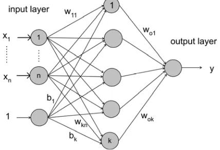
An ANN can be defined as a processing system consisting of a large number of simple, highly interconnected processing element (neurons) in an architecture inspired by the structure of the human brain [4]. An ANN is characterized by its architecture, learning algo-rithm and activations function. The architecture describes the connections between the neurons. It consists of, generally, an input layer, an output layer and adequate number of hidden layers in between. The layers in the network are interconnected by links that associated with weight that dictate the effect on the information passing through them. These weights are updated by learning algorithm. The activation function relates the output of a neuron to its input. The most commonly used activation functions are: threshold, piece-wise linear, sigmoid and Gaussian function. . Figure 1 shows a single artificial neuron, where wji is the weight values and f is activation function.
Figure 1. A Single Artificial Neuron
Table 1. Activation Functions
Type of Activation Function
The learning process of the neural network can be likened to the way a child learns to recognize patterns, shapes and sounds, and discerns among them. For example, the child has to be exposed to a number of examples of a particular type of tree for her to be able to recognize that type of tree latter on. In addition, the child has to be exposed to different types of trees for her to be able to differentiate among trees.
The human brain has the uncanny ability to recognize and comprehend various patterns. The neural network is extremely primitive in this aspect. The network’s strength, however, is in its ability to comprehend and discern subtle patterns in a large number of variables at a time without being stifled by detail. It can also carry out multiple operations simultaneously. Not only can it identify patterns in a few variables, it also can detect correlations in hundreds of variables. It is this feature of the network that is particularly suitable in analyzing relationships between a large numbers of market variables. The networks can learn from experience. They can cope with “fuzzy” patterns – patterns that are difficult to reduce to precise rules. They can also be retrained and thus can adapt to changing market behavior.
The network holds particular promise for econometric applications. Multilayer feed for-ward neural networks as a common type of neural network with appropriate parameters are capable of approximating a large number of diverse functions arbitrarily well [5]. Even when a data set is noisy or has irrelevant inputs, the networks can learn important features of the data. Inputs that may appear irrelevant may in fact contain useful information. The promise of neural networks lies in their ability to learn patterns in a complex signal.
Recently, there are at least two most popular ANN in various applications, namely multilayer feed forward network (MFN) and radial basis function network (RBFN). ANN has been popular because of its capability as general approximate of nonlinear process. Multilayer feed forward network with back propagation learning algorithm is used in this paper. This type of ANN is shown in Figure 2.
Figure 2. A Typical Multilayer Feed Forward Neural Network
and the output of the network by
∑
== k
i
i i
o h
w y
1
) .
( …..(2)
The learning process of ANN is carried out using input-output data to update the weights and biases. One of the technique used to obtain these parameter is back propagation algorithm [4,6]. The weight adjustment is done iteratively from the output layer backward to previous layers to achieve a minimum mean square error (MSE) between the network output and the desired output [4]. The number of iterations is often termed as epoch.
The back propagation algorithm can be summarized as follows. Suppose a MFN is trained by gradient descent to approximate an unknown function, based on some training data consisting of pairs (x,t). The vector x represents a pattern of input to the network, and the vector
t the corresponding target (desired output). The overall gradient with respect to the entire training set is just the sum of the gradients for each pattern; then it is described how to compute the gradient for just a single training pattern. Let’s number the units, and denote the weight from unit j to unit i by wij.
a. Definitions:
the error signal for unit j:
the (negative)
gradient for weight wij:
the set of nodes
anterior to unit i:
the set of nodes
posterior to unit j:
b. The gradient. The gradient is expanded into two factors by use of the chain rule:
The first factor is the error of unit i. The second is
Putting the two together, we get
.
To compute this gradient, we thus need to know the activity and the error for all relevant nodes in the network.
c. Forward activaction. The activity of the input units is determined by the network's external input x. For all other units, the activity is propagated forward:
Note that before the activity of unit i can be calculated, the activity of all its anterior nodes (forming the set Ai) must be known. Since feedforward networks do not contain cycles, there is an ordering of nodes from input to output that respects this condition.
d. Calculating output error. Assuming that the sum-squared loss is used.
e. Error back propagation. For hidden units, the error is back propagated from the output nodes (hence the name of the algorithm). Again using the chain rule, we can expand the error of a hidden unit in terms of its posterior nodes:
Of the three factors inside the sum, the first is just the error of node i. The second is
while the third is the derivative of node j's activation function:
For hidden units h that use the tanh activation function, we can make use of the special identity
tanh(u)' = 1 - tanh(u)2, giving
Putting all the pieces together, yields
The common steps in ANN learning process are as follows.
a. Input collection and preprocessing of the input data (if necessary). This includes the number of sampled data and data normali-zation.
b. Determining the structure of the ANN. Including number of inputs, neurons, hidden layers and activation functions.
c. Training the ANN, using the input pattern and desired output.
d. Validation of the trained ANN.
2. Artificial Neural Network For Time Series Forecasting
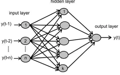
The ability of ANN to discover nonlinear relationships in input data makes them ideal for modeling nonlinear time series. Therefore, ANN can be used to predict future values in a time series based on current and historical data. This can be considered as univariate modeling of time series. Figure 3 shows the typical network for time series forecasting.
Figure 3. Multilayer Feed Forward Network for Time Series Forecasting
hap-pens when the ANN has poor generalization capability or the data used is limited to small number. The ANN has memorized the training examples but it has not learned to generalize the new input pattern in prediction. This is because what so called over fitting occurs during the training. The error on the training set is driven to a very small value, but when new data is presented to the network the error is large.
One method to improve generalization capability is called early stopping. In this tech-nique the available data is divided into three subsets. The first subset is the training set, which is used for computing the gradient and updating the network weights and biases. The second subset is the validation set. The error on the validation set is monitored during the training process. The validation error will normally decrease during the initial phase of training, as does the training set error. However, when the network begins to over fit the data, the error on the validation set will typically begin to rise. When the validation error increases for a specified number of iterations, the training is stopped, and the weights and biases at the minimum of the validation error are returned [7].
3. Autoregressive Integrated Moving Average (ARIMA)
It is a forecasting model using combination of three components, namely: Firstly, autoregres-sive term. It may use first order or higher order AR terms. Each AR relates to the use of a lagged value of the residual in the forecasting equation for the unconditional residual. Sec-ondly, integration orders term. Each integration order corresponds to differencing series being forecast. First order integration means that the forecasting model is designed to the first difference of the original series. Lastly is the Moving Average term. Moving Average
forecasting model which is using lagged values of the forecast error is to improve the current forecast.
This ARIMA method consists of four steps [8] (1). Identification. This first steps is to identify the lagged value of the autoregressive term the order of integrated and the moving average term. (2). Estimation. The next step is to estimate the parameter of the autoregressive and moving average term. This can be done by the simple least squares.(3). Diagnostic check-ing. This is to see whether the chosen model fits the data reasonably well. (4). Forecasting. After considering all the steps, finally, we use the model to make a forecasting.
RESEARCH METHOD
The number of available monthly data of Islamic banking deposit (saving) is 143. It starts from January 1994 up to November 2005. The data can be downloaded from Bank Negara Malaysia Website. About the first 75 percent data is used for training and the last 25 percent data is forecasted by the ANN and ARIMA.
next one step. This is carried out iteratively until 33 times prediction. The training was specified to achieve MSE of 10-5.
The training phase has usually no much problem. The problem is when new input pat-tern fed to the ANN to predict the new value. Early stopping plays an important role here to improve generalization capability.
FINDINGS AND DISCUSSION
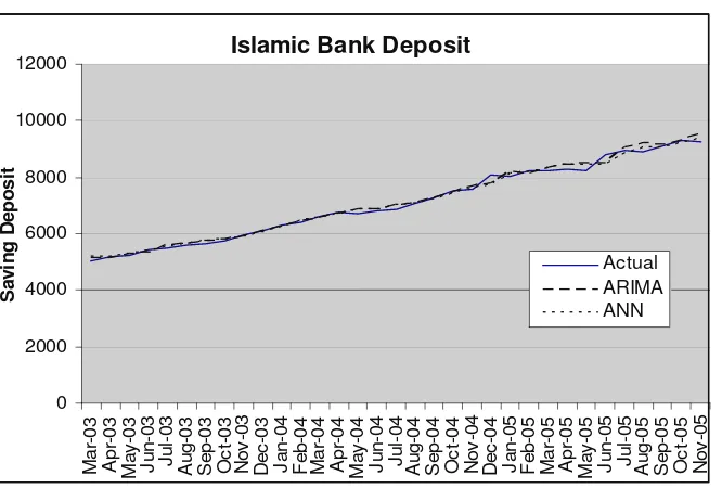
The plots comparing the actual index and the forecasting result by ANN with early stopping technique and ARIMA is shown in Figures 4. From the plot, it can be seen that the ANN has shown a good capability for time series fore-casting based on historical data of Malaysia Islamic banking deposit. The proposed method of ANN was also able to forecast the pattern with low error.
The corellogram is used to test whether the data is stationary or not for ARIMA. It shows that the data is not stationary in the level form,
but it is stationary in the first difference. After considering the requirement needed for estimating the model, using least square regression, we come up with the model below:
Deposit = 30.29168 + 0.84512* Deposit (-1) + 0.195871*Deposit (-7)
To see the accuracy between these two method (ANN and ARIMA), we compute the error for each forecasting tools. In doing this, we employ the Mean Absolute Percentage Error (MAPE).
CONCLUSION
Forecasting is very important for decision maker to have an idea of what might occur in the future. We, in this paper, have tried to implement two method for forecasting, namely Artificial Neural Network (ANN) and Autore-gressive Integrated Moving Average (ARIMA). The result shows that ANN can be used as an alternative prediction tool that produces a slightly better performance than ARIMA. MAPE for ANN is 1.3 and for ARIMA is 1.38 and there is no statistical pre-analysis of the data needed to obtain the significant lag used like in ARIMA. Furthermore, ANN can be used for multiple-ahead prediction tool as well. Thus, short term and long term forecasting is also subject for ANN research.
REFERENCES
Daniel, C.P.C., Wei, N.C., Lek, T.H.. 1999.
Using Neural Network to Forecast For-eign Exchange Rate. Nanyang Techno-logical University.
Gujarati, D. 2003. Basic Econometric. Inter-national Edition, 4th ed”, New York: Mcgraw hill.
Hamid, S.A. 2004. Primer on Using Neural Networks for Forecasting Market Vari-ables. Working Paper, No. 2004-03, Southern New Hampshire University.
Hansen, James V., Ray D. Nelson, 2003, Time-Series Analysis with Neural Networks and ARIMA-Neural Network Hybrids,
Journal of Experimental & Theoretical Artificial Intelligence, Vol. 15, No. 3, July, pp. 315-330.
Ho, S.L.; Xie M.; Goh T.N, 2002, A Comparative Study of Neural Network
and Box-Jenkins ARIMA modeling in Time Series Prediction, Computers and Industrial Engineering, Vol. 42, No. 2, 11 April, pp. 371-375(5)
Kolarik, T., Rudorfer., G, 1994. Time Series Forecasting using Neural Network. Time Series and Neural Network, APL, 1994.
Kumar, S. 2004. Neural Networks: a Classroom Approach. New Delhi: Tata - Mc. Graw Hill.
Lin, C.T., and Lee, G.C.S., 1996. Neural Fuzzy Systems. A Synergism to Intelligent System. New Jersey: Prentice-Hall. 1996.
Nelson, M., Hill, T., Remus, W., & O'Connor, M. (1999). Time series forecasting using neural networks: should the data be deseasonalized first? Journal of Forecasting, 18, 359-367.
Neural Network Toolbox User’s Guide. 2001. the MathWorks, Inc.
Pai, Ping-Feng dan Chih-Sheng Lin, 2005, A Hybrid Arima and Support Vector Machines Model in Stock Price Forecasting, Omega Journal, Vol. 33, No. 6, December, pp. 497-505.