El e c t ro n ic
Jo ur
n a l o
f P
r o
b a b il i t y
Vol. 16 (2011), Paper no. 20, pages 552–586. Journal URL
http://www.math.washington.edu/~ejpecp/
Collision local time of transient random walks and
intermediate phases in interacting stochastic systems
∗
Matthias Birkner
1, Andreas Greven
2, Frank den Hollander
3 4Abstract
In a companion paper[6], a quenched large deviation principle (LDP) has been established for the empirical process of words obtained by cutting an i.i.d. sequence of letters into words ac-cording to a renewal process. We apply this LDP to prove that the radius of convergence of the generating function of the collision local time of two independent copies of a symmetric and strongly transient random walk onZd, d≥ 1, both starting from the origin, strictly increases
when we condition on one of the random walks, both in discrete time and in continuous time. We conjecture that the same holds when the random walk is transient but not strongly transient. The presence of these gaps implies the existence of anintermediate phasefor the long-time be-haviour of a class of coupled branching processes, interacting diffusions, respectively, directed polymers in random environments .
Key words: Random walks, collision local time, annealed vs. quenched, large deviation princi-ple, interacting stochastic systems, intermediate phase.
AMS 2000 Subject Classification:Primary 60G50, 60F10, 60K35, 82D60.
Submitted to EJP on December 24, 2008, resubmitted upon invitation to EJP on March 27, 2010, final version accepted January 11, 2011.
1Institut für Mathematik, Johannes-Gutenberg-Universität Mainz, Staudingerweg 9, 55099 Mainz, Germany.
Email:[email protected]
2Mathematisches Institut, Universität Erlangen-Nürnberg, Bismarckstrasse 11
2, 91054 Erlangen, Germany.
Email:[email protected]
3Mathematical Institute, Leiden University, P.O. Box 9512, 2300 RA Leiden, The Netherlands.
Email:[email protected]
4EURANDOM, P.O. Box 513, 5600 MB Eindhoven, The Netherlands
∗This work was supported in part by DFG and NWO through the Dutch-German Bilateral Research Group “Mathematics
1
Introduction and main results
In this paper, we derivevariational representations for the radius of convergence of the generating
functions of the collision local time of two independent copies of a symmetric and transient random walk, both starting at the origin and running in discrete or in continuous time, when the average is taken w.r.t. one, respectively, two random walks. These variational representations are subsequently used to establish the existence of an intermediate phase for the long-time behaviour of a class of interacting stochastic systems.
1.1
Collision local time of random walks
1.1.1 Discrete time
LetS= (Sk)∞k=0 andS′= (S′k)∞k=0 be two independent random walks onZd, d≥1, both starting at
the origin, with anirreducible,symmetricandtransienttransition kernelp(·,·). Writepnfor then-th convolution power ofp, and abbreviatepn(x):=pn(0,x), x ∈Zd. Suppose that
lim
n→∞
logp2n(0)
logn =:−α, α∈[1,∞). (1.1)
WritePto denote the joint law ofS,S′. Let
V =V(S,S′):=
∞ X
k=1
1{S
k=S′k} (1.2)
be thecollision local timeofS,S′, which satisfiesP(V <∞) =1 by transience, and define
z1 := sup
¦
z≥1: EzV |S<∞ S-a.s.©, (1.3)
z2 := sup¦z≥1: EzV<∞©. (1.4)
The lower indices indicate the number of random walks being averaged over. Note that, by the tail triviality ofS, the range ofz’s for whichE[zV |S]converges isS-a.s. constant.1
Let E := Zd, let Ee = ∪n∈NEn be the set of finite words drawn from E, and let Pinv(Ee N
) denote
the shift-invariant probability measures on EeN, the set of infinite sentences drawn from Ee. Define
f: Ee→[0,∞)via
f((x1, . . . ,xn)) =
pn(x1+· · ·+xn)
p2⌊n/2⌋(0) [2 ¯G(0)−1], n∈N, x1, . . . ,xn∈E, (1.5)
where ¯G(0) =P∞n=0p2n(0)is the Green function at the origin associated with p2(·,·), which is the transition matrix ofS−S′, and p2⌊n/2⌋(0)>0 for alln∈Nby the symmetry ofp(·,·). The following variational representations hold forz1andz2.
1Note thatP(V=
Theorem 1.1. Assume(1.1). Then z1=1+exp[−r1], z2=1+exp[−r2]with
r1 ≤ sup
Q∈Pinv(eEN )
¨Z
e
E
(π1Q)(d y)logf(y)−Ique(Q)
«
, (1.6)
r2 = sup
Q∈Pinv(eEN)
¨Z
e
E
(π1Q)(d y)logf(y)−Iann(Q)
«
, (1.7)
where π1Q is the projection of Q onto E, while Ie que and Iann are the rate functions in the quenched, respectively, annealed large deviation principle that is given in Theorem2.2, respectively,2.1below with (see(2.4),(2.7)and(2.13–2.14))
E=Zd, ν(x) =p(x), x∈E, ρ(n) =p2⌊n/2⌋(0)/[2 ¯G(0)−1], n∈N. (1.8)
Let
Perg,fin(EeN) ={Q∈ Pinv(eEN): Qis shift-ergodic,mQ<∞}, (1.9)
where mQ is the average word length underQ, i.e., mQ =
R e
E(π1Q)(y)τ(y)with τ(y)the length
of the word y. Theorem 1.1 can be improved under additional assumptions on the random walk,
namely,2
P
x∈Zd
kxkδp(x)<∞ for someδ >0, (1.10)
lim inf
n→∞
log[pn(S
n)/p2⌊n/2⌋(0) ]
logn ≥0 S−a.s., (1.11)
inf
n∈N
Elog[pn(Sn)/p2⌊n/2⌋(0) ]>−∞. (1.12)
Theorem 1.2. Assume(1.1)and(1.10–1.12). Then equality holds in(1.6), and
r1 = sup
Q∈Perg,fin(eEN )
¨Z
e
E
(π1Q)(d y)logf(y)−Ique(Q)
«
∈R, (1.13)
r2 = sup
Q∈Perg,fin(eEN )
¨Z
e
E
(π1Q)(d y)logf(y)−Iann(Q)
«
∈R. (1.14)
In Section 6 we will exhibit classes of random walks for which (1.10–1.12) hold. We believe that (1.11–1.12) actually hold in great generality.
BecauseIque≥Iann, we haver1≤r2, and hencez2≤z1(as is also obvious from the definitions ofz1
andz2). We prove that strict inequality holds under the stronger assumption that p(·,·)isstrongly transient, i.e.,P∞n=1npn(0)<∞. This excludesα∈(1, 2)and part ofα=2 in (1.1).
Theorem 1.3. Assume(1.1). If p(·,·)is strongly transient, then1<z2<z1≤ ∞. 2By the symmetry of p(
·,·), we have supx∈Zdp
n(x)
≤ p2⌊n/2⌋(0) (see (3.15)), which implies that sup
n∈Nsupx∈Zd
SinceP(V = k) = (1−F¯)F¯k, k∈N∪ {0}, with ¯F :=P ∃k∈N: Sk = Sk′, an easy computation givesz2=1/F¯. But ¯F=1−[1/G¯(0)](see Spitzer[27], Section 1), and hence
z2=G¯(0)/[G¯(0)−1]. (1.15)
Unlike (1.15), no closed form expression is known for z1. By evaluating the function inside the
supremum in (1.13) at a well-chosenQ, we obtain the following upper bound.
Theorem 1.4. Assume(1.1)and(1.10–1.12). Then
z1≤1+
X
n∈N e−h(pn)
!−1
<∞, (1.16)
where h(pn) =−Px∈Zdpn(x)logpn(x)is the entropy of pn(·).
There are symmetric transient random walks for which (1.1) holds withα=1. Examples are any
transient random walk onZin the domain of attraction of the symmetric stable law of index 1 on
R, or any transient random walk onZ2in the domain of (non-normal) attraction of the normal law
onR2. If in this situation (1.10–1.12) hold, then the two threshold values in (1.3–1.4) agree.
Theorem 1.5. If p(·,·)satisfies(1.1)withα=1and(1.10–1.12), then z1=z2.
1.1.2 Continuous time
Next, we turn the discrete-time random walks S and S′ into continuous-time random walks eS =
(St)t≥0 andSe′= (eS′
t)t≥0 by allowing them to make steps at rate 1, keeping the same p(·,·). Then
the collision local time becomes
e
V :=
Z ∞
0
1{eS
t=eS′t}d t. (1.17)
For the analogous quantitiesez1 andez2, we have the following.3
Theorem 1.6. Assume(1.1). If p(·,·)is strongly transient, then1<ez2<ez1≤ ∞.
An easy computation gives
logez2=2/G(0), (1.18)
whereG(0) =P∞n=0pn(0)is the Green function at the origin associated with p(·,·). There is again no simple expression forez1.
Remark 1.7. An upper bound similar to(1.16)holds forze1as well. It is straightforward to show that z1<∞andez1<∞as soon as p(·)has finite entropy.
3For a symmetric and recurrent random walk again triviallyze
1.1.3 Discussion
Our proofs of Theorems 1.3–1.6 will be based on the variational representations in Theorem 1.1–1.2. Additional technical difficulties arise in the situation where the maximiser in (1.7) has infinite mean
word length, which happens precisely when p(·,·)is transient but not strongly transient. Random
walks with zero mean and finite variance are transient for d ≥ 3 and strongly transient for d ≥5
(Spitzer[27], Section 1).
Conjecture 1.8. The gaps in Theorems1.3 and 1.6are present also when p(·,·) is transient but not strongly transient providedα >1.
In a 2008 preprint by the authors (arXiv:0807.2611v1), the results in[6]and the present paper were
announced, including Conjecture 1.8. Since then, partial progresshas been made towards settling
this conjecture. In Birkner and Sun[7], the gap in Theorem 1.3 is proved for simple random walk
onZd,d≥4, and it is argued that the proof is in principle extendable to a symmetric random walk
with finite variance. In Birkner and Sun [8], the gap in Theorem 1.6 is proved for a symmetric
random walk onZ3 with finite variance in continuous time, while in Berger and Toninelli [1]the
gap in Theorem 1.3 is proved for a symmetric random walk onZ3 in discrete time under a fourth
moment condition.
The role of the variational representation for r2 is not to identify its value, which is achieved in
(1.15), but rather to allow for acomparisonwithr1, for which no explicit expression is available. It
is an open problem to prove (1.11–1.12) under mild regularity conditions onS. Note that the gaps
in Theorems 1.3–1.6 do not require (1.10–1.12).
1.2
The gaps settle three conjectures
In this section we use Theorems 1.3 and 1.6 to prove the existence of an intermediate phase for
three classes of interacting particle systems where the interaction is controlled by a symmetric and
transient random walk transition kernel. 4
1.2.1 Coupled branching processes
A.Theorem 1.6provesa conjecture put forward in Greven[17],[18]. Consider a spatial population
model, defined as the Markov process (ηt)t≥0, with η(t) = {ηx(t): x ∈ Zd} where ηx(t) is the
number of individuals at site x at time t, evolving as follows:
(1) Each individual migrates at rate 1 according toa(·,·).
(2) Each individual gives birth to a new individual at the same site at rateb.
(3) Each individual dies at rate(1−p)b.
(4) All individuals at the same site die simultaneously at ratep b.
4In each of these systems the case of a symmetric and recurrent random walk is trivial and no intermediate phase is
Here,a(·,·)is an irreducible random walk transition kernel onZd×Zd, b∈(0,∞)is a birth-death
rate, p∈[0, 1]is a coupling parameter, while (1)–(4) occur independently at every x ∈Zd. The
case p = 0 corresponds to a critical branching random walk, for which the average number of
individuals per site is preserved. The case p>0 is challenging because the individuals descending
from different ancestors are no longer independent.
A critical branching random walk satisfies the followingdichotomy(where for simplicity we restrict
to the case wherea(·,·)is symmetric): if the initial configurationη0 is drawn from a shift-invariant
and shift-ergodic probability distribution with a positive and finite mean, thenηt as t → ∞locally
dies out (“extinction”) when a(·,·) is recurrent, but converges to a non-trivial equilibrium (“sur-vival”) whena(·,·)istransient, both irrespective of the value ofb. In the latter case, the equilibrium has the same mean as the initial distribution and has all moments finite.
For the coupled branching process with p > 0 there is a dichotomy too, but it is controlled by a
subtle interplayofa(·,·), b andp: extinction holds when a(·,·)isrecurrent, but also whena(·,·) is
transientandpissufficiently large. Indeed, it is shown in Greven[18]that ifa(·,·)is transient, then there is a uniquep∗∈(0, 1]such that survival holds forp<p∗and extinction holds forp>p∗.
Recall the critical valuesez1,ez2introduced in Section 1.1.2. Then survival holds ifE(exp[bpVe]|eS)<
∞Se-a.s., i.e., ifp<p1 with
p1=1∧(b−1logez1). (1.19)
This can be shown by a size-biasing of the population in the spirit of Kallenberg[23]. On the other
hand, survival with afinite second momentholds if and only ifE(exp[bpVe])<∞, i.e., if and only if
p<p2with
p2=1∧(b−1logez2). (1.20)
Clearly, p∗≥p1≥p2. Theorem 1.6 shows that ifa(·,·)satisfies (1.1) and is strongly transient, then
p1>p2, implying that there is an intermediate phase of survival with aninfinite second moment.
B. Theorem 1.3 corrects an error in Birkner [3], Theorem 6. Here, a system of individuals living
on Zd is considered subject to migration and branching. Each individual independently migrates
at rate 1 according to a transient random walk transition kernela(·,·), and branches at a rate that depends on the number of individuals present at the same location. It is argued that this system has an intermediate phase in which the numbers of individuals at different sites tend to an equilibrium with a finite first moment but an infinite second moment. The proof was, however, based on a
wrong rate function. The rate function claimed in Birkner[3], Theorem 6, must be replaced by that
in[6], Corollary 1.5, after which the intermediate phase persists, at least in the case where a(·,·) satisfies (1.1) and is strongly transient. This also affects[3], Theorem 5, which uses[3], Theorem
6, to computez1in Section 1.1 and finds an incorrect formula. Theorem 1.4 shows that this formula
actually is an upper bound forz1.
1.2.2 Interacting diffusions
Theorem 1.6 proves a conjecture put forward in Greven and den Hollander [19]. Consider the
system X = (X(t))t≥0, with X(t) = {Xx(t): x ∈ Zd}, of interacting diffusions taking values in
[0,∞)defined by the following collection of coupled stochastic differential equations:
d Xx(t) = X
y∈Zd
a(x,y)[Xy(t)−Xx(t)]d t+pbXx(t)2 dW
Here, a(·,·)is an irreducible random walk transition kernel on Zd×Zd, b ∈(0,∞)is a diffusion constant, and (W(t))t≥0 withW(t) = {Wx(t): x ∈ Zd} is a collection of independent standard
Brownian motions onR. The initial condition is chosen such thatX(0)is a invariant and
shift-ergodic random field with a positive and finite mean (the evolution preserves the mean). Note that,
even thoughX a.s. has non-negative paths when starting from a non-negative initial conditionX(0),
we prefer to writeXx(t)as
p
Xx(t)2 in order to highlight the fact that the system in (1.21) belongs
to a more general family of interacting diffusions with Hölder-1
2 diffusion coefficients, see e.g.[19],
Section 1, for a discussion and references.
It was shown in[19], Theorems 1.4–1.6, that ifa(·,·)issymmetricandtransient, then there exist 0< b2≤b∗such that the system in (1.21) locally dies out when b>b∗, but converges to an equilibrium when 0< b< b∗, and this equilibrium has afinite second moment when 0< b< b2 and aninfinite second momentwhen b2 ≤ b < b∗. It was shown in[19], Lemma 4.6, that b∗≥ b∗∗=logez1, and
it was conjectured in[19], Conjecture 1.8, that b∗> b2. Thus, as explained in[19], Section 4.2, if
a(·,·)satisfies (1.1) and is strongly transient, then this conjecture is correct with
b∗≥logez1 > b2=logez2. (1.22)
Analogously, by Theorem 1.1 in[8]and by Theorem 1.2 in[7], the conjecture is settled for a class
of random walks in dimensionsd=3, 4 including symmetric simple random walk (which ind=3, 4
is transient but not strongly transient).
1.2.3 Directed polymers in random environments
Theorem 1.3disprovesa conjecture put forward in Monthus and Garel[25]. Leta(·,·)be a symmet-ric and irreducible random walk transition kernel onZd×Zd, letS= (Sk)∞k=0 be the corresponding
random walk, and let ξ = {ξ(x,n): x ∈ Zd,n ∈ N} be i.i.d. R-valued non-degenerate random
variables satisfying
λ(β):=logE exp[βξ(x,n)]∈R ∀β∈R. (1.23)
Put
en(ξ,S):=exp
Xn
k=1
βξ(Sk,k)−λ(β)
, (1.24)
and set
Zn(ξ):=E[en(ξ,S)] = X
s1,...,sn∈Zd
n
Y
k=1
p(sk−1,sk)
en(ξ,s), s= (sk)∞k=0,s0=0, (1.25)
i.e., Zn(ξ)is the normalising constant in the probability distribution of the random walkS whose
paths are reweighted by en(ξ,S), which is referred to as the “polymer measure”. The ξ(x,n)’s
describe a random space-time medium with whichS is interacting, withβ playing the role of the
interaction strength or inverse temperature.
It is well known thatZ= (Zn)n∈Nis a non-negative martingale with respect to the family of
sigma-algebrasFn:=σ(ξ(x,k),x ∈Zd, 1≤k≤n),n∈N. Hence
lim
with the event {Z∞ = 0} being ξ-trivial. One speaks of weak disorder if Z∞ > 0 ξ-a.s. and of
strong disorder otherwise. As shown in Comets and Yoshida[12], there is a unique critical value
β∗∈[0,∞] such that weak disorder holds for 0≤ β < β∗ and strong disorder holds for β > β∗. Moreover, in the weak disorder region the paths have a Gaussian scaling limit under the polymer measure, while this is not the case in the strong disorder region. In the strong disorder region the paths are confined to a narrow space-time tube.
Recall the critical valuesz1,z2 defined in Section 1.1. Bolthausen[9]observed that
EZ2
n
=E
h
exp{λ(2β)−2λ(β)}Vn
i
, withVn:=
n
X
k=1
1{Sk=S′k}, (1.27)
whereSandS′are two independent random walks with transition kernelp(·,·), and concluded that
ZisL2-bounded if and only ifβ < β2 withβ2∈(0,∞]the unique solution of
λ(2β2)−2λ(β2) =logz2. (1.28)
SinceP(Z∞>0)≥E[Z∞]2/E[Z∞2]andE[Z∞] =Z0=1 for an L2-bounded martingale, it follows that β < β2 implies weak disorder, i.e.,β∗≥ β2. By a stochastic representation of the size-biased
law ofZn, it was shown in Birkner[4], Proposition 1, that in fact weak disorder holds ifβ < β1 with β1∈(0,∞]the unique solution of
λ(2β1)−2λ(β1) =logz1, (1.29)
i.e.,β∗≥β1. Sinceβ7→λ(2β)−2λ(β)is strictly increasing for any non-trivial law for the disorder
satisfying (1.23), it follows from (1.28–1.29) and Theorem 1.3 that β1 > β2 when a(·,·) satisfies
(1.1) and is strongly transient and when ξ is such that β2 < ∞. In that case the weak disorder
region contains a subregion for whichZ isnot L2-bounded. This disproves a conjecture of Monthus
and Garel[25], who argued thatβ2=β∗.
Camanes and Carmona[10]consider the same problem for simple random walk and specific choices
of disorder. With the help of fractional moment estimates of Evans and Derrida[16], combined with
numerical computation, they show thatβ∗> β2for Gaussian disorder ind≥5, for Binomial disorder
with small mean ind≥4, and for Poisson disorder with small mean ind≥3.
See den Hollander[21], Chapter 12, for an overview.
Outline
Theorems 1.1, 1.3 and 1.6 are proved in Section 3. The proofs need only assumption (1.1). Theo-rem 1.2 is proved in Section 4, TheoTheo-rems 1.4 and 1.5 in Section 5. The proofs need both assumptions (1.1) and (1.10–1.12)
In Section 2 we recall the LDP’s in [6], which are needed for the proof of Theorems 1.1–1.2 and
their counterparts for continuous-time random walk. This section recalls the minimum from [6]
2
Word sequences and annealed and quenched LDP
Notation. We recall the problem setting in [6]. Let E be a finite or countable set of letters. Let
e
E = ∪n∈NEn be the set of finite words drawn from E. Both E and Ee are Polish spaces under the
discrete topology. Let P(EN) and P(EeN) denote the set of probability measures on sequences
drawn fromE, respectively,Ee, equipped with the topology of weak convergence. Writeθ andθefor
the left-shift acting onEN, respectively,EeN. WritePinv(EN
),Perg(EN
)andPinv(EeN
),Perg(EeN
)for the set of probability measures that are invariant and ergodic underθ, respectively,θe.
Forν ∈ P(E), letX = (Xi)i∈Nbe i.i.d. with lawν. Forρ∈ P(N), letτ= (τi)i∈Nbe i.i.d. with law
ρhaving infinite support and satisfying thealgebraic tail property
lim
n→∞
ρ(n)>0
logρ(n)
logn =:−α, α∈[1,∞). (2.1)
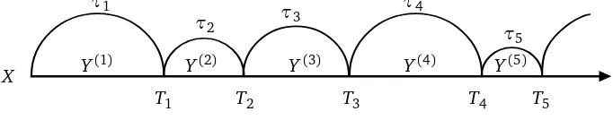
(No regularity assumption is imposed on supp(ρ).) Assume thatX andτare independent and write
Pto denote their joint law. Cut words out ofX according toτ, i.e., put (see Fig. 1)
T0:=0 and Ti:=Ti−1+τi, i∈N, (2.2)
and let
Y(i):= XTi
−1+1,XTi−1+2, . . . ,XTi
, i∈N. (2.3)
Then, under the lawP, Y = (Y(i))i∈N is an i.i.d. sequence of words with marginal lawqρ,ν on eE
given by
qρ,ν (x1, . . . ,xn)
:=P Y(1)= (x1, . . . ,xn)
=ρ(n)ν(x1)· · ·ν(xn), n∈N, x1, . . . ,xn∈E.
(2.4)
τ1
τ2 τ3
τ4
τ5
T1 T2 T3 T4 T5 Y(1) Y(2) Y(3) Y(4) Y(5) X
Figure 1: Cutting words from a letter sequence according to a renewal process.
Annealed LDP.ForN ∈N, let(Y(1), . . . ,Y(N))per be the periodic extension of (Y(1), . . . ,Y(N))to an element ofEeN, and define
RN := 1
N
NX−1
i=0
δθei(Y(1),...,Y(N))per ∈ Pinv(Ee N
), (2.5)
theempirical process of N -tuples of words. The following large deviation principle (LDP) is standard
(see e.g. Dembo and Zeitouni[14], Corollaries 6.5.15 and 6.5.17). Let
H(Q|q⊗ρ,Nν):= lim
N→∞
1
Nh
Q|
FN
(q⊗ρ,Nν)|
FN
be thespecific relative entropy of Q w.r.t. qρ⊗,Nν, whereFN = σ(Y(1), . . . ,Y(N)) is the sigma-algebra
generated by the first N words, Q|
FN is the restriction of Q to FN, and h(· | ·) denotes relative
entropy (defined for probability measuresϕ,ψon a measurable spaceF ash(ϕ|ψ) =R
Flog dϕ
dψdϕ
if the density dϕ
dψ exists and as∞otherwise).
Theorem 2.1. [Annealed LDP] The family of probability distributionsP(RN ∈ ·), N ∈N, satisfies
the LDP onPinv(eEN)with rate N and with rate function Iann: Pinv(EeN)→[0,∞]given by
Iann(Q) =H(Q|qρ⊗,Nν). (2.7)
The rate function Iannis lower semi-continuous, has compact level sets, has a unique zero at Q=q⊗ρ,Nν, and is affine.
Quenched LDP.To formulate the quenched analogue of Theorem 2.1, we need some further
nota-tion. Letκ:EeN→ENdenote theconcatenation mapthat glues a sequence of words into a sequence
of letters. ForQ∈ Pinv(EeN)such that mQ:=EQ[τ1]<∞(recall thatτ1 is the length of the first
word), defineΨQ∈ Pinv(EN
)as
ΨQ(·):= 1
mQEQ
τX1−1
k=0
δθkκ(Y)(·)
. (2.8)
Think ofΨQ as the shift-invariant version of the concatenation of Y under the law Q obtained after
randomising the location of the origin.
For tr∈N, let[·]tr: eE→[Ee]tr:=∪trn=1Endenote theword length truncationmap defined by
y = (x1, . . . ,xn)7→[y]tr:= (x1, . . . ,xn∧tr), n∈N, x1, . . . ,xn∈E. (2.9)
Extend this to a map fromeENto[Ee]N tr via
(y(1),y(2), . . .)tr:= [y(1)]tr,[y(2)]tr, . . ., (2.10)
and to a map fromPinv(EeN)toPinv([eE]Ntr)via
[Q]tr(A):=Q({z∈eEN: [z]tr∈A}), A⊂[Ee]Ntr measurable. (2.11)
Note that ifQ∈ Pinv(EeN
), then[Q]tris an element of the set
Pinv,fin(EeN) ={Q∈ Pinv(eEN): mQ<∞}. (2.12)
Theorem 2.2. [Quenched LDP, see[6], Theorem 1.2 and Corollary 1.6](a) Assume(2.1). Then, forν⊗N
–a.s. all X , the family of (regular) conditional probability distributionsP(RN ∈ · |X), N ∈N,
satisfies the LDP on Pinv(EeN) with rate N and with deterministic rate function Ique: Pinv(EeN) → [0,∞]given by
Ique(Q):=
Ifin(Q), if Q∈ Pinv,fin(EeN), lim
tr→∞I fin [Q]
tr
where
Ifin(Q):=H(Q|qρ⊗,Nν) + (α−1)mQH(ΨQ|ν⊗
N
). (2.14)
The rate function Ique is lower semi-continuous, has compact level sets, has a unique zero at Q=q⊗ρ,Nν, and is affine. Moreover, it is equal to the lower semi-continuous extension of Ifin fromPinv,fin(EeN)to
Pinv(EeN).
(b) In particular, if(2.1)holds withα=1, then forν⊗N
–a.s. all X , the familyP(RN ∈ · |X)satisfies
the LDP with rate function Ianngiven by(2.7).
Note that the quenched rate function (2.14) equals the annealed rate function (2.7) plus an
addi-tional term that quantifies the deviation ofΨQ from the reference lawν⊗Non the letter sequence.
This term is explicit whenmQ<∞, but requires a truncation approximation whenmQ=∞.
We close this section with the following observation. Let
Rν:=
Q∈ Pinv(EeN): w−lim
L→∞
1
L
L−1
X
k=0
δθkκ(Y)=ν⊗
N
Q−a.s.
. (2.15)
be the set ofQ’s for whichthe concatenation of words has the same statistical properties as the letter sequence X. Then, forQ∈ Pinv,fin(eEN), we have (see[6], Equation (1.22))
ΨQ=ν⊗N ⇐⇒ Ique(Q) =Iann(Q) ⇐⇒ Q∈ Rν. (2.16)
3
Proof of Theorems 1.1, 1.3 and 1.6
3.1
Proof of Theorem 1.1
The idea is to put the problem into the framework of (2.1–2.5) and then apply Theorem 2.2. To that end, we pick
E:=Zd, eE=ÝZd :=∪
n∈N(Zd)n, (3.1)
and choose
ν(u):=p(u), u∈Zd, ρ(n):= p
2⌊n/2⌋(0)
2 ¯G(0)−1, n∈N, (3.2)
where
p(u) =p(0,u),u∈Zd, pn(v−u) =pn(u,v),u,v∈Zd, G¯(0) =
∞ X
n=0
p2n(0), (3.3)
the latter being the Green function ofS−S′at the origin.
Recalling (1.2), and writing
zV= (z−1) +1V =1+
V
X
N=1
(z−1)N
V
N
(3.4)
with
V N
= X
0<j1<···<jN<∞
1{S
we have
the number of random walks being averaged over.)
The notation in (3.1–3.2) allows us to rewrite the first formula in (3.7) as
FN(1)(X) = X
Note that, sinceÝZd carries the discrete topology, f is trivially continuous.
LetRN ∈ Pinv((ÝZd)N) be the empirical process of words defined in (2.5), andπ1RN ∈ P(ÝZd)the
projection ofRN onto the first coordinate. Then we have
FN(1)(X) =E
wherePis the joint law ofX andτ(recall (2.2–2.3)). By averaging (3.10) overX we obtain (recall
Indeed, the Fourier representation ofpn(x,y)reads
pn(x) = 1 (2π)d
Z
[−π,π)d
d k e−i(k·x)bp(k)n (3.14)
withbp(k) =Px∈Zdei(k·x)p(0,x). Becausep(·,·)is symmetric, we havebp(k)∈[−1, 1], and it follows
that
max
x∈Zdp
2n(x) =p2n(0), max x∈Zdp
2n+1(x)
≤p2n(0), ∀n∈N. (3.15)
Consequently, f((x1, . . . ,xn)) ≤ [2 ¯G(0)−1] is bounded from above. Therefore, by applying the
annealedLDP in Theorem 2.1 to (3.11), in combination with Varadhan’s lemma (see Dembo and Zeitouni[14], Lemma 4.3.6), we getz2=1+exp[−r2]with
r2:= lim
N→∞
1
NlogF
(2)
N ≤ sup Q∈Pinv((ZÝd)N
)
¨Z
Ý Zd
(π1Q)(d y)logf(y)−Iann(Q)
«
= sup
q∈P(ZÝd)
¨Z
Ý Zd
q(d y)logf(y)−h(q|qρ,ν)
« (3.16)
(recall (1.3–1.4) and (3.6)). The second equality in (3.16) stems from the fact that, on the set of
Q’s with a given marginalπ1Q=q, the functionQ7→Iann(Q) =H(Q|q⊗ N
ρ,ν)has a unique minimiser
Q = q⊗N
(due to convexity of relative entropy). We will see in a moment that the inequality in (3.16) actually is an equality.
In order to carry out the second supremum in (3.16), we use the following.
Lemma 3.1. Let Z:=P
y∈ZÝd f(y)qρ,ν(y). Then
Z
Ý Zd
q(d y)logf(y)−h(q|qρ,ν) =logZ−h(q|q∗) ∀q∈ P(ÝZd), (3.17)
where q∗(y):= f(y)qρ,ν(y)/Z, y∈ÝZd.
Proof. This follows from a straightforward computation.
Inserting (3.17) into (3.16), we see that the suprema are uniquely attained atq=q∗andQ=Q∗=
(q∗)⊗N, and thatr2≤logZ. From (3.9) and (3.12), we have
Z=X
n∈N
X
x1,...,xn∈Zd
pn(x1+· · ·+xn)
n
Y
k=1
p(xk) =X
n∈N
p2n(0) =G¯(0)−1, (3.18)
where we use that Pv∈Zdpm(u+v)p(v) = pm+1(u), u∈Zd, m ∈N, and recall that ¯G(0) is the
Green function at the origin associated withp2(·,·). Henceq∗is given by
q∗(x1, . . . ,xn) =
pn(x1+· · ·+xn) ¯
G(0)−1
n
Y
k=1
Moreover, sincez2 =G¯(0)/[G¯(0)−1], as noted in (1.15), we see thatz2 =1+exp[−logZ], i.e.,
r2=logZ, and so indeed equality holds in (3.16).
The quenched LDP in Theorem 2.2, together with Varadhan’s lemma applied to (3.8), gives z1 = 1+exp[−r1]with
r1:= lim
N→∞
1
NlogF
(1)
N (X)≤ sup Q∈Pinv((ZÝd)N
)
¨Z
Ý Zd
(π1Q)(d y)logf(y)−Ique(Q)
«
X−a.s., (3.20)
where Ique(Q) is given by (2.13–2.14). Without further assumptions, we are not able to reverse
the inequality in (3.20). This point will be addressed in Section 4 and will require assumptions (1.10–1.12).
3.2
Proof of Theorem 1.3
To compare (3.20) with (3.16), we need the following lemma, the proof of which is deferred.
Lemma 3.2. Assume (1.1). Let Q∗ = (q∗)⊗N
with q∗ as in (3.19). If mQ∗ < ∞, then Ique(Q∗) >
Iann(Q∗).
With the help of Lemma 3.2 we complete the proof of the existence of the gap as follows. Since
logf is bounded from above, the function
Q7→
Z
Ý Zd
(π1Q)(d y)logf(y)−Ique(Q) (3.21)
is upper semicontinuous. Therefore, by compactness of the level sets of Ique(Q), the function in
(3.21) achieves its maximum at someQ∗∗that satisfies
r1=
Z
Ý Zd
(π1Q∗∗)(d y)logf(y)−Ique(Q∗∗)≤
Z
Ý Zd
(π1Q∗∗)(d y)logf(y)−Iann(Q∗∗)≤r2. (3.22)
Ifr1=r2, thenQ∗∗=Q∗, because the function
Q7→
Z
Ý Zd
(π1Q)(d y)logf(y)−Iann(Q) (3.23)
hasQ∗as its unique maximiser (recall the discussion immediately after Lemma 3.1). ButIque(Q∗)> Iann(Q∗)by Lemma 3.2, and so we have a contradiction in (3.22), thus arriving atr1<r2.
In the remainder of this section we prove Lemma 3.2.
Proof. Note that
q∗((Zd)n) = X
x1,...,xn∈Zd
pn(x1+· · ·+xn) ¯
G(0)−1
n
Y
k=1
p(xk) = p
2n(0)
¯
G(0)−1, n∈N, (3.24)
and hence, by assumption (1.2),
lim
n→∞
logq∗((Zd)n)
and
implying the claim becauseα∈(1,∞)(recall (2.14)).
In order to verify (3.27), we compute the first two marginals ofΨQ∗. Using the symmetry ofp(·,·),
There are many p(·,·)’s for which (3.29) fails, and for these (3.27) holds. However, for simple
random walk (3.29) does not fail, because a 7→ p2n−1(a) is constant on the 2d neighbours of the
origin, and so we have to look at the two-dimensional marginal.
and
This shows that consecutive letters are not uncorrelated underΨQ∗, and implies that (3.27) holds as
claimed.
3.3
Proof of Theorem 1.6
The proof follows the line of argument in Section 3.2. The analogues of (3.4–3.7) are
where the conditioning in the first expression in (3.37) is on the full continuous-time path Se =
♮ is the discrete-time random walk with transition
kernel p(·,·) and(Jt)t≥0 is the rate-1 Poisson process on[0,∞), and then average over the jump times of(Jt)t≥0 while keeping the jumps ofX♮fixed. In this way we reduce the problem to the one
for the discrete-time random walk treated in the proof of Theorem 1.6. For the first expression in
(3.38) thispartial annealinggives an upper bound, while for the second expression it is simply part
of the averaging overeS. together with the critical values
r1♮:= lim To this end write out
we may rewrite (3.44) as
This expression is similar in form as the first line of (3.8), except that the order of the ji’s is not strict. However, defining
and recalling (3.41), we therefore have the relation
r1♮ =loghΘ0(0) +ebr1♮
Equations (3.51–3.52) replace (3.8–3.9). We can now repeat the same argument as in (3.16–
3.22), with the sole difference that f in (3.9) is replaced by f♮ in (3.52), and this, combined with
Lemma 3.3 below, yields the gapr1♮ <r2♮.
We first check that f♮ is bounded from above, which is necessary for the application of Varadhan’s
lemma. To that end, we insert the Fourier representation (3.14) into (3.45) to obtain
Next we note that
indeed is bounded from above.
Note that X♮ is the discrete-time random walk with transition kernel p(·,·). The key ingredient
behindbr1♮<br2♮ is the analogue of Lemma 3.2, this time withQ∗= (q∗)⊗N
replacing (3.19). The proof is deferred to the end.
Lemma 3.3. Assume (1.1). Let Q∗ = (q∗)⊗N
with q∗ as in (3.56). If mQ∗ < ∞, then Ique(Q∗) >
Iann(Q∗).
This shows thatbr1♮ <br2♮ via the same computation as in (3.21–3.23). The analogue of (3.18) reads
Z♮=X
where we use (3.37), (3.39), (3.42), (3.50) and (3.57).
We close by proving Lemma 3.3.
Proof. We must adapt the proof in Section 3.2 to the fact that q∗ has a slightly different form, namely, pn(x1+· · ·+xn)is replaced by Θn(x1+· · ·+xn), which averages transition kernels. The
computations are straightforward and are left to the reader. The analogues of (3.24) and (3.26) are
while the analogues of (3.31–3.32) are
q∗(x1=a) = 1 p(a)
2G(0)−Θ0(0) 1 2
∞ X
k=0
pk(a)[1−2−k−1] =1 2p(a)
G(a)−Θ0(a)
1
2G(0)−Θ0(0)
,
q∗ {(a,b)} ×(Zd)n−2= 1 p(a)p(b)
2G(0)−Θ0(0) ∞ X
m=0
pn−2+m(a+b)2−n−m−1
n+m
m
.
(3.60)
Recalling (3.30), we find
ΨQ∗(a,−a)−p(a)2>0, (3.61)
implying thatΨQ∗6=ν⊗N(recall (3.2)), and henceH(ΨQ∗|ν⊗N)>0, implying the claim.
4
Proof of Theorem 1.2
This section uses techniques from[6]. The proof of Theorem 1.2 is based on two approximation
lemmas, which are stated in Section 4.1. The proof of these lemmas is given in Sections 4.2–4.3.
4.1
Two approximation lemmas
Return to the setting in Section 2. For Q ∈ Pinv(EeN
), let H(Q) denote the specific entropy ofQ. Writeh(· | ·)andh(·)to denote relative entropy, respectively, entropy. Write, and recall from (1.9),
Perg(EeN) ={Q∈ Pinv(eEN): Qis shift-ergodic},
Perg,fin(EeN) ={Q∈ Pinv(eEN): Qis shift-ergodic,mQ<∞}. (4.1)
Lemma 4.1. Let g: eE→Rbe such that
lim inf
k→∞
g X|(0,k]
logk ≥0forν
⊗N
−a.s.all X with X|(0,k]:= (X1, . . . ,Xk). (4.2)
Let Q∈ Perg,fin(EeN
)be such that H(Q)<∞and G(Q):=Re
E(π1Q)(d y)g(y)∈R. Then
lim inf
N→∞
1
N logE
exp
N
Z
e
E
(π1RN)(d y)g(y)
X
≥G(Q)−Ique(Q)forν⊗N–a.s. all X. (4.3)
Lemma 4.2. Let g: eE→Rbe such that
sup
k∈N
Z
Ek
|g (x1, . . . ,xk)
|ν⊗k(d x1, . . . ,d xk)<∞. (4.4)
Let Q∈ Perg(EeN)be such that Ique(Q)<∞and G(Q)∈R. Then there exists a sequence(Qn)n∈Nin
Perg,fin(eEN
)such that
lim inf
n→∞ [G(Qn)−I que(Q
n)]≥G(Q)−Ique(Q). (4.5)
Moreover, if E is countable andν satisfies
∀µ∈ P(E): h(µ|ν)<∞=⇒h(µ)<∞, (4.6)
Lemma 4.2 immediately yields the following.
Corollary 4.3. If g satisfies(4.4)andν satisfies(4.6), then
sup
With Corollary 4.3, we can now complete the proof of Theorem 1.2.
Proof. Return to the setting in Section 3.1. In Lemma 4.1, pickg=logf with f as defined in (3.9). Then (1.11) is the same as (4.2), and so it follows that
lim inf
where the condition that the first term under the supremum be finite is redundant becauseg=logf
is bounded from above (recall (3.13)). Recalling (3.10) and (3.20), we thus see that
r1≥ sup To remove this restriction, we use Corollary 4.3. First note that, by (1.12), condition (4.4) in
Lemma 4.2 is fulfilled for g = logf. Next note that, by (1.10) and Remark 4.4 below, condition
(4.6) in Lemma 4.2 is fulfilled forν = p. Therefore Corollary 4.3 implies thatr1 equals the
right-hand side of (1.13), and that the suprema in (1.13) and (1.6) agree.
Equality (1.14) follows easily from the fact that the maximiser of the right-hand side of (1.7) is given byQ∗= (q∗)⊗Nwithq∗defined in (3.19), as discussed after Lemma 3.1: IfmQ∗ <∞, then we
are done, otherwise we approximateQ∗via truncation.
for someC ∈(0,∞). Therefore
h(µ) =X
x∈Z
µ(x)log
1
µ(x)
= X
x∈Z
µ(x)≤(e+|x|)−2
µ(x)log
1
µ(x)
+ X
x∈Z
µ(x)>(e+|x|)−2
µ(x)log
1
µ(x)
≤ X
x∈Z
2 log(e+|x|)
(e+|x|)2 +2
X
x∈Z
µ(x)log(e+|x|)<∞,
(4.11)
where the last inequality uses (4.10).
4.2
Proof of Lemma 4.1
Proof. The idea is to make the first word so long that it ends in front of the first region inX that
looks like the concatenation ofN words drawn fromQ, and after that cutN “Q-typical” words from
this region. Condition (4.2) ensures that the contribution of the first word to the left-hand side of (4.3) is negligible on the exponential scale.
To formalise this idea, we borrow some techniques from[6], Section 3.1. Let H(ΨQ) denote the
specific entropy of ΨQ (defined in (2.8)), and Hτ|κ(Q) the “conditional specific entropy of word
lengths under the lawQgiven the concatenation” (defined in[6], Lemma 1.7). We need the relation
H(Q|q⊗ρ,Nν) =mQH(ΨQ|ν⊗N)−Hτ|κ(Q)−EQlogρ(τ1)
. (4.12)
First, we note that H(Q) < ∞ and mQ < ∞ imply that H(ΨQ) < ∞ and Hτ|κ(Q) < ∞ (see [6],
Lemma 1.7). Next, we fixǫ >0. Following the arguments in[6], Section 3.1, we see that for allN
large enough we can find a finite setA =A(Q,ǫ,N)⊂ EeN of “Q-typical sentences” such that, for allz= (y(1), . . . ,y(N))∈ A, the following hold:
1
N
N
X
i=1
logρ(|yi|)∈hEQlogρ(τ1)
−ǫ,EQlogρ(τ1)
+ǫi,
1
N log
{z′∈ A: κ(z′) =κ(z)}∈hHτ|κ(Q)−ǫ,Hτ|κ(Q) +ǫi,
1
N
N
X
i=1
g(y(i))∈hG(Q)−ǫ,G(Q)−ǫi.
(4.13)
Put B := κ(A) ⊂ Ee. We can choose A in such a way that the elements of B have a length in
N(mQ−ǫ),N(mQ+ǫ). Moreover, we have
P X begins with an element ofB≥exp−Nχ(Q), (4.14)
where we abbreviate
χ(Q):=mQH(ΨQ|ν⊗N) +ǫ. (4.15)
Put
τN:=min
i∈N: θiXbegins with an element ofB . (4.16)
Then, by (4.14) and the Shannon-McMillan-Breiman theorem, we have
lim sup
N→∞
1
Indeed, for eachN, coarse-grainX into blocks of lengthLN :=⌊N(mQ+ǫ)⌋. Fori∈N∪ {0}, letAN,i
where we use (2.13–2.14), (4.12) and (4.15). Finally, letǫ↓0 to get the claim.
4.3
Proof of Lemma 4.2
Proof. Without loss of generality we may assume thatmQ=∞, for otherwiseQn≡Qsatisfies (4.5).
level tr ∈N, let Qνtr be the law obtained from Q by replacing all words of length ≥ tr by words of
while under [Q]tr they do not. The proof is straightforward but lengthy, and is deferred to
Ap-pendix A.
On the other hand, we have
Z
where we use dominated convergence for the first summand and condition (4.4) for the second
summand. Combining (4.25–4.26), we see that we can choose tr=tr(n)such that (4.5) holds for
Moreover, for allℓ <tr andk=1, . . . ,ℓ,
h
LQν tr Y
(1)
k |τ1=ℓ
|ν≤h
LQν tr Y
(1) |τ1=ℓ
|ν⊗ℓ=h
LQ Y(1)|τ1=ℓ
|ν⊗ℓ. (4.29)
Combine (4.28–4.29) with (4.6) to conclude that all the summands in (4.27) are finite.
5
Proof of Theorems 1.4 and 1.5
Proof of Theorem 1.4. Letq∈ P(ZÝd)be given by
q(x1, . . . ,xn):=ρ¯(n)ν(x1)· · ·ν(xn), n∈N, x1, . . . ,xn∈Zd, (5.1)
for some ¯ρ ∈ P(N) withPn∈Nnρ¯(n)< ∞, and letQ = q⊗ N
. Then Q is ergodic, mQ <∞, and
(recall (2.4))
Ique(Q) =H q⊗N|(qρ,ν)⊗ N
=h(ρ¯|ρ) (5.2)
becauseΨQ=ν⊗N
. Now pick tr∈N, ¯ρ= [ρ∗]tr withρ∗given by
ρ∗(n):= 1
Z exp[−h(p
n)], n
∈N, Z:= X
n∈N
exp[−h(pn)], (5.3)
ν(·) =p(·), and compute (recall (3.2) and (3.9))
Z
Ý Zd
(π1Q)(d y)logf(y) =
Z
Ý Zd
q(d y)logf(y)
= X
n∈N
X
x1,...,xn∈Zd
¯
ρ(n)p(x1)· · ·p(xn)log
pn(x
1+· · ·+xn)
ρ(n)
= X
n∈N
¯
ρ(n) [−logρ(n)−h(pn)]
=logZ+X
n∈N
¯
ρ(n)log
ρ∗(n)
ρ(n)
=logZ+h ρ¯|ρ−h ρ¯|ρ∗.
(5.4)
Then (1.13), (5.2) and (5.4) give the lower bound
r1≥logZ−h ρ¯|ρ∗. (5.5)
Let tr→ ∞, to obtainr1≥logZ, which proves the claim (recall thatz1=1+exp[−r1]).
It is easy to see that the choice in (5.3) is optimal in the class ofq’s of the form (5.1) withν(·) =p(·). By using (3.15), we see thath(p2n)≥ −logp2n(0)andh(p2n+1)≥ −logp2n(0). Hence Z <∞by the transience ofp(·,·).
6
Examples of random walks satisfying assumptions (1.10–1.12)
In this section we exhibit classes of random walks for which (1.10–1.12) hold.
1. Let S be an irreducible symmetric random walk on Zd with E[kS1k3] < ∞. Then standard
cumulant expansion techniques taken from Bhattacharya and Ranga Rao[2]can be used to show
that for everyC1∈(0,∞)there is aC2∈(0,∞)such that
pn(x) = c
nd/2exp
h
− 1
2n(x,Σ
−1x)i1+O(logn)
C2 n1/2
,
n→ ∞, kxk ≤pC1nlog logn, pn(x)>0,
(6.1)
whereΣis the covariance matrix ofS1(which is assumed to be non-degenerate), andcis a constant
that depends on p(·). The restrictionpn(x)> 0 is necessary: e.g. for simple random walk x and
nin (6.1) must have the same parity. The Hartman-Wintner law of the iterated logarithm (see e.g.
Kallenberg[24], Corollary 14.8), which only requiresS1to have mean zero and finite variance, says
that
lim sup
n→∞
|(Sn)i|
p
2Σiinlog logn
=1 a.s., i=1, . . . ,d, (6.2)
where(Sn)i is the i-th component ofSn. UsingkSnk ≤pdmax1≤i≤d|(Sn)i|, we obtain that there is aC3∈(0,∞)such that
lim sup
n→∞
kSnk
p
nlog logn≤
C3 S−a.s. (6.3)
Combining and (6.1) and (6.3), we find that there is aC4∈(0,∞)such that
log[pn(Sn)/p2⌊n/2⌋(0) ]≥ −C4kSnk2/n ∀n∈N S−a.s. (6.4)
Combining (6.3) and (6.4), we get (1.11).
To get (1.12), we argue as follows. Note thatE(S1) =0 andE(kS1k2)<∞. Forn∈N, we have
X
x∈Zd
pn(x)log[pn(x)/p2⌊n/2⌋(0)] =:Σ1(n) + Σ2(n), (6.5)
where the sums run over, respectively,
I1(n):={x∈Zd: pn(x)/p2⌊n/2⌋(0)≥exp[−n−1kxk2−1]},
I2(n):={x∈Zd: pn(x)/p2⌊n/2⌋(0)<exp[−n−1kxk2−1]}.
(6.6)
We have
Σ1(n)≥ X
x∈Zd
pn(x) [−n−1kxk2−1] =−E(kS1k2)−1. (6.7)
Sinceu7→uloguis non-increasing on the interval[0,e), we also have
Σ2(n)≥ X
x∈Zd
for some C5 ∈(0,∞). By the local central limit theorem, we havep2⌊n/2⌋(0)∼ C6n−d/2 asn→ ∞
for someC6 ∈(0,∞). HenceΣ1(n) + Σ2(n)is bounded away from−∞uniformly inn∈N, which
proves (1.12).
2.LetSbe a symmetric random walk onZthat is in the normal domain of attraction of a symmetric
stable law with indexa∈(0, 1)and suppose that the one-step distribution is regularly varying, i.e.,
P(S1=x) = [1+o(1)]C|x|−1−a,|x| → ∞for someC∈(0,∞). Then, as shown e.g. in Chover[13]
and Heyde[20],
|Sn| ≤n1/a(logn)1/a+o(1) a.s. n→ ∞. (6.9)
psatisfies (1.1) withα=1/a ∈(1,∞), the standard local limit theorem gives (see e.g. Ibragimov
and Linnik[22], Theorem 4.2.1)
pn(x) = [1+o(1)]n−1/af(x n−1/a), |x|/n1/a=O(1), (6.10)
with f the density of the stable law. The remaining region was analysed in Doney[15], Theorem A,
namely,
pn(x) = [1+o(1)]C n|x|−1−a, |x|/n1/a→ ∞. (6.11) In fact, the proof of (6.11) shows that forKsufficiently large there existc∈(0,∞)andn0∈Nsuch that
c−1≤ p
n(x)
n|x|−1−a ≤c, n≥n0,|x| ≥K n
1/a. (6.12)
Combining (6.9–6.11), we get
log[pn(Sn)/p2⌊n/2⌋(0) ]≥[−(1+a)/a+o(1)]log logn a.s., (6.13)
which proves (1.11).
To get (1.12), we argue as follows. Pick K and c such that (6.12) holds. Obviously, it suffices to
check (1.12) with the infimimum overNrestricted ton≥ n0. Because f is uniformly positive and
bounded on[−K,K], (6.11) gives
inf
n≥n0
X
|x|≤K n1/a
pn(x)log[pn(x)/p2⌊n/2⌋(0) ]≥log
inf
y∈[−K,K]f(y)/2
>−∞. (6.14)
Applying (6.10) top2⌊n/2⌋(0)and (6.11) topn(x)we obtain
X
|x|>K n1/a
pn(x)log[pn(x)/p2⌊n/2⌋(0) ]≥ −c1 X
|x|>K n1/a
1
n1/a |x|/n
1/a−1−a
(1+a)log c2|x|/n1/a
(6.15)
for somec1,c2∈(0,∞). The right-hand side is an approximating Riemann sum for the integral
−2c1(1+a)
Z ∞
K
d y y−1−alog(c2y)>−∞. (6.16)
3.For an example similar to2.leading toα=1 in (1.1), letpbe a symmetric transition probability
onZsatisfying