El e c t ro n ic
Jo ur n
a l o
f P
r o b
a b i l i t y
Vol. 12 (2007), Paper no. 2, pages 47–74. Journal URL
http://www.math.washington.edu/~ejpecp/
A Compensator Characterization of Point Processes
on Topological Lattices
∗B. Gail Ivanoff†
Dept. of Mathematics and Statistics University of Ottawa
P.O. Box 450, Stn. A Ottawa ON K1N 6N5
CANADA [email protected]
Ely Merzbach‡ Dept. of Mathematics
Bar-Ilan University 52900 Ramat-Gan
ISRAEL
Mathieu Plante P.O.Box 3595 Banff, AB T1L 1E2
CANADA
mathieu plante [email protected]
Abstract
We resolve the longstanding question of how to define the compensator of a point process on a general partially ordered set in such a way that the compensator exists, is unique, and characterizes the law of the process. We define a family of one-parameter compensators and prove that this family is unique in some sense and characterizes the finite dimensional distributions of a totally ordered point process. This result can then be applied to a general point process since we prove that such a process can be embedded into a totally ordered point process on a larger space. We present some examples, including the partial sum ∗This paper is dedicated to the memory of our friend and colleague, Andr´e Robert Dabrowski (1955-2006). †Research supported by a grant from the Natural Sciences and Engineering Research Council of Canada. ‡Work done while visiting the University of Ottawa. The second author thanks G. Ivanoff for her characteristic
multiparameter process, single line point processes, multiparameter renewal processes, and obtain a new characterization of the two-parameter Poisson process.
Key words: point process, compensator, partial order, single jump process, partial sum process, adapted random set, renewal process, Poisson process, multiparameter martingale. AMS 2000 Subject Classification: Primary 60K05, 60G55, 60G48.
1
Introduction
When working on the dynamical properties of a point process defined on a partially ordered space, one of the main tools is thecompensator: the unique predictable increasing process which compensates the point process, i.e. the difference between the point process and the compensator is a martingale. In the classical case, a remarkable result of J. Jacod in (9) established that the law (i.e. the finite dimensional distributions) of a simple point process on the real line is characterized by the knowledge of its compensator. The power of martingale methods in the statistical analysis of point processes on R+ is well-established, and some of these techniques
have recently been extended to point processes on more general spaces in (7).
In this paper, we provide a positive answer to the question of whether such a characterization exists for general point processes on partially ordered sets. It is clear that for such processes, this problem becomes much more complicated and has remained open except in special cases (cf. (5), (6)). First, compensators can be defined in several ways for any simple point process, depending on how one defines the “history” or “past” at a point. As well, only under stringent conditions can one prove existence and uniqueness of the compensator. Moreover, even if we have a compensator that is unique in some sense, it will not generally characterize the law of the point process. To illustrate this, we recall an example studied in detail in (6).
Suppose our parameter set T is the positive quadrant of the plane R2+, let τ = (τ1, τ2) be
process possesses several compensators depending on the information available at t about the random pointτ (i.e. the “history” at t). Three of them are the following:
Λwt = property with respect to the relevant history, and in each case, Λ· is predictable in some sense. The history at tconsists of the values ofNs for allsinAtfor Λw, to the left oft for Λ1, below
tfor Λ2, and inDt for Λ∗. SinceT is in this example a product space, we observe thatNt can
be viewed as a marked point process on R+ (τ1 is interpreted as the time of the jump and τ2
as the mark), so according to Jacod’s (9) characterization result, the law ofN is determined by Λ1 (or Λ2, by symmetry). In other words, we can reconstruct the distribution G. However, as is well known from multivariate survival analysis, neither the ratio G(dt)/G(Act) nor the ratio
G(dt)/G(Dc
t) (thehazard function) determinesG, so neither Λw nor Λ∗ can characterize the law
In this example, the compensator Λ1 does the job. However, it works only because T has a product structure (as required for Jacod’s marked point process approach). Moreover, at
t = (t1, t2) this compensator requires complete information about N to the left of t1 (i.e. in
A1t) or by symmetry, below t2 (A2t). In survival analysis, this means that one needs the entire
sample in one direction to estimate the value of the distribution function G at t. However, in practice it may happen that the only information available at time t = (t1, t2) ∈T consists of
the locations of jumps inAt={s∈T :s≤t}.
Another example is the Poisson process M = {Mt, t ∈ R2+}. As is explained in (5), since the
increments are independent each of the compensators of M is a deterministic function and in fact at each pointt, it is the measure of the rectangleAt(up to a constant). In this special case,
the compensator Λ∗ has been shown to characterize the Poisson process (cf. (6), Theorem 5.3.1) whereas Λw does not. The compensator Λ∗ works well if it is deterministic (for example, it also characterizes the set-indexed Brownian motion among the class of square integrable continuous multiparameter strong martingales ((6), Theorem 5.2.1)), but as observed above, it fails for other processes such as the single jump process.
Here, we resolve the open question by defining the compensator of a general point processN on an arbitrary topological lattice T in such a way that it always exists, is unique, and completely characterizes the law ofN. T need not have the product structure required for Jacod’s marked point process approach, and in the case of the single jump process or more generally, point processes whose jumps are strictly increasing, the only information required at timet∈T is the location of jumps in At ={s ∈ T : s≤ t}. For more general point processes, the information
required at t is the location of any jump point τ for which N(Aτ) ≤ N(At). In fact, the
compensator will be defined to be a class of (one-dimensional) compensators of point processes onR+generated by projections ofN alongflows (increasing maps fromR+to a class of subsets
of T). We show that the projection of a point process along a flow is a one-parameter point process, and therefore the compensator of the projection is well defined. As will be explained later in full detail, this compensator will be called “U −flow compensator” . This approach was first introduced by Plante in (11) in the special case T = R2+. Notice that our new flow compensator is not identifiable with any of the compensators Λw, Λ1 or Λ∗.
In addition to the theoretical interest of this result, there are important areas of application such as multiparameter renewal theory and survival analysis (see (7) and (8)). In addition, we give a new characterization of the Poisson process on the plane.
The paper is organized as follows. In Section 2, we develop all the prerequisites needed for point processes on a partially ordered parameter set. We define strictly simple point processes in a very general framework using the concept of flow and we discuss how this allows us to exploit results from classical one-parameter theory. In Section 3, we study point processes whose jump points are totally ordered. The flow compensator is defined for flows on the original space T
embedded process. Therefore, we get a complete compensator characterization for any strictly simple point process. In Section 5, we present more examples. In particular, we investigate the single line process and apply it to two special cases: the renewal point process and the Poisson point process on the plane. We obtain a new characterization of the Poisson process and compare it to a similar result given by Aletti and Capasso in (1).
2
Prerequisites
The point processes are defined on a complete separable metric space (T, d). We will require thatT be partially ordered.
Assumption 2.1. T is endowed with a partial order “≤” for whichT is a complete distributive lattice (i.e. every subset of T has a sup and an inf, and for u, s, t∈T,
u∨(s∧t) = (u∨s)∧(u∨t)) and u∧(s∨t) = (u∧s)∨(u∧t).)
In particular,T contains a minimum element denoted by0and a maximum element denoted by
1. This setup includes compact rectangles in Rp+ with the usual partial order and we shall use [0,1]2 as the fundamental example to illustrate our approach.
Fort∈T, the partial order generates the following sets:
At := ↓t={s∈T :s≤t}
Et := ↑t={s∈T :s≥t}
We observe that As∧t=As∧At andEs∨t=Es∧Et,∀s, t,∈T.
Assumption 2.2. For every t∈T, both At and Et are d-closed.
Now we introduce the “dyadics” inT. The notation “s < t” should be interpreted as “s≤t and
s6=t”.
Assumption 2.3. The partial order on T is sufficiently rich that there exists an increasing sequence of finite sublattices(Tn)ofT each containing0and1, such that for anyt∈T, t6=0,1,
each open neighbourhood oftcontains pointst′, t′′∈Tndistinct fromtsuch thatt′< t < t′′. Each
open neighbourhood of 0 (respectively, 1) contains a pointt′ ∈T
n distinct from0 (respectively,
1). The elements of Tn can be thought of as the dyadics of order n.
In particular, defining
t+n :=∧t′∈T n;t≤t′t
′ andt−
n :=∨t′∈T n;t′≤tt
′,
it follows thatt=∧nt+n = limnt+n = limnt−n =∨nt−n, and any pointt can therefore be
approx-imated from above (respectively, below) by elements in Tn either as an infimum (respectively,
supremum) or as a limit in the metric d.
Assumptions 2.1-2.3 suffice for the results in Section 3; for Section 4, a further mild assumption will be required.
1. For u, s, t∈T, d(s∧u, t∧u)≤d(s, t) and d(s∨u, t∨u)≤d(s, t). 2. The sublattices Tn of Assumption 2.3 can be chosen so that
lim
n supt∈T d(t, t +
n) = 0 and limn sup t∈T
d(t, t−n) = 0.
Comment 2.5. IfT is bounded, then it is reasonable to suppose thatT has a maximum element and thatTn is finite. This is not a restriction if there exists an increasing sequence of bounded
subsets B1 ⊆B2 ⊆ ...⊆T, such that T = ∪∞n=1Bn and each subset Bn satisfies the preceding
assumptions. The law of any point process on T is expressed in terms of its finite dimensional distributions on bounded Borel subsets of T (cf. (3), pg.166), and so it suffices to characterize the law of the point process on eachBn. This allows us to extend our results to point processes
on Rd+, for example.
We now define the left neighbourhoods Cnassociated withTn:
C ∈ Cn if and only ifC =Ctn:=At\ ∪t′∈T
n,t′6≥tAt′ for somet∈Tn.
The sequence (Cn) is a nested sequence of finite partitions of T that ultimately separates the
points ofT, and so forms a dissecting system. Consequently, any closed setK can be expressed as
K=∩n(∪t∈KCtn).
Each of the unions in the expression above is finite sinceCn is finite. As a result, the Borel sets
of T are generated by the sets{At:t∈ ∪nTn}.
We say that two sets A, B ⊂T are incomparable if a and b are incomparable for every a∈ A
and b∈B.
Proposition 2.6. If t, t′ ∈Tn are incomparable, then Ctn andCtn′ are incomparable sets.
Proof. This is an easy consequence of the observation that by definition,Ctn∩At′ =Cn
t′∩At=∅
when t, t′ are incomparable. ✷
We now turn to point processes onT. LetN denote the set of finite integer-valued measuresµ
onT withµ({x}) = 0 or 1 for allx∈T andµ({0}) = 0. LetF(N) be the smallestσ-algebra on
N with respect to which the mappingsµ→µ(At) are measurable, for everyt∈T. For C∈ Cn,
µ(C) can be calculated as a finite linear combination of random variables µ(At), t∈ Tn. Since
∪nCn is a semiring which generates the Borel sets in T, by Proposition A.2.5.IV of (3), F(N)
coincides with theσ-algebra generated by the topology of weak convergence onN.
Definition 2.7. A point process N is a measurable mapping from a probability space (Ω,F, P) into (N,F(N)).
Assumption 2.3 ensures that the law of a point process is uniquely determined by its finite dimensional distributions of the form P(N(At1) =k1, ..., N(Atj) =kj) for t1, ..., tj ∈ Tn, some
n. Hence, equivalently the law is determined by the finite dimensional distributions ofN on the left-neighbourhoods Cn, for everyn.
Notice that our definition automatically ensures that there is at most one jump point at any
Definition 2.8. A flow f on T is a continuous strictly increasing map from[0,1] toT (i.e., if
s < t, then f(s)< f(t)).
Given any finite totally ordered subset t0 < t1 < t2 < ... < tn of T, Assumptions 2.3 and 2.4
ensure that there exists a flow f connecting t0, ..., tn: that is, there exist points 0 =u0 < u1 <
... < un= 1 such thatf(ui) =ti, i= 0, ..., n. This can be proven in a manner similar to that of
Theorem 5.1.6 in (6).
Given a flow f, we can define the projection Nf of a point process N along the flow: Nf is an
integer-valued process on [0,1] defined by
Nf(u) :=N(Af(u)), u∈[0,1].
AlthoughNf can be regarded as an (integer-valued) point measure on [0,1], it is not necessarily the case thatNf is a simple point process.
Definition 2.9. A point process N on T is strictly simple if for any finite totally ordered subset 0 =t0 < t1 < t2 < ... < tm of ∪nTn, there exists a flow f connecting t0, ..., tm such that Nf is
a simple point process on [0,1]. Denote by FN any countable class of flows containing at least
one flow f connecting each finite totally ordered subset of ∪nTn and such that Nf is simple.
As an example, consider T = [0,1]2 endowed with the usual partial order. A point process N
on T is strictly simple if and only if there is at most one jump point ofN on any horizontal or vertical line. FN includes all continuous increasing mapsf : [0,1]→[0,1] that are increasing in
only one component at a time: i.e. the trajectory off is continuous, consisting of horizontal and vertical line segments. Formally, ifu <1 andf(u) = (f1(u), f2(u)) then∃ǫ >0 such that either
f1(u) =f1(u+δ) ∀δ ∈ (0, ǫ) or f2(u) =f2(u+δ) ∀δ ∈(0, ǫ). We note that not all flows yield
simple projections ifN has more than one jump point. For example, consider the point process
N with jumps at (14,12) and (12,14). N is strictly simple since Nf is simple for every f ∈ F N.
However, consider the flowf defined byf(u) = (u, u),0≤u≤1. In this case Nf is not simple, sinceNf({12}) = 2.
We now consider a simple point processN defined on the unit interval. LetFN = (FN(u) :u∈
[0,1]) = (σ{N(v) : 0≤v≤u};u ∈[0,1]) be the minimal filtration generated byN and denote by ΛN the compensator ofN with respect toFN (i.e. the unique predictable increasing process
in the Doob-Meyer decomposition ofN). According to the now classic result of Jacod (9), the law ofN is uniquely characterized by ΛN.
As discussed in Section 1, there is no obvious definition for the compensator of a point process on a general poset since there is no unique way of defining the Doob-Meyer decomposition, and none of the known compensators characterize the law (for a more detailed discussion see (6)). We will instead see that flows enable us to exploit Jacod’s one dimensional characterization. The first step is to consider point processes whose jumps are totally ordered; we do this in the next section (§3). We shall see in §4 that in fact this is enough to permit us to handle general point processes.
3
Totally ordered point processes
t
t
t
t
τ1
τ2
τ4
τ3
t0
t4
t3
t2
t1
C1 C2
C3 C4
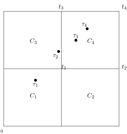
Figure 1: A totally ordered point process
{x :µ({x}) = 1} is totally ordered (see Figure 1, for example). Such processes have a special structure that allow us to identify the law of N given the laws of Nf, f ∈ FN; the following
theorem is the key result. Here we give only a sketch of the proof; the complete proof may be found in Appendix A.
Theorem 3.1. Let (T, d) be a complete separable metric space satisfying Assumptions 2.1, 2.2 and 2.3. LetN be a totally ordered point process onT and letF be any class of flows containing at least one flow connecting each finite totally ordered subset of∪nTn. The law ofN determines
and is determined by the laws of the family of the projected point processes Nf, f ∈F.
Proof. (Sketch) It is trivial that the law ofNf is determined by the law ofN. For the converse, we assume that the laws of Nf are known for every f ∈ F and it is enough to show that we
can reconstruct the finite dimensional distributions of N on the sets in Cn; i.e. if Tn = (t0 =
0, t1, ..., tjn =1) and Ci=C
n
ti, we must be able to find
P(N(C1) =k1, ..., N(Cjn) =kjn)
from the laws ofNf, f ∈F. The crucial point behind the proof is that if t
i and tj are
incom-parable, then so are Ci and Cj. Consequently, when N is totally ordered, at most one of any
collection of incomparable sets can contain any jump points. Below we give an illustration of how this simple fact is used.
Consider the unit squareT = [0,1]2 and the sublattice consisting of the pointst
0 = (0,0), t1 =
(12,12), t2 = (1,12), t3 = (12,1), t4 = (1,1). The corresponding left neighbourhoodsCi =Cti are illustrated in Figure 1, along with a realization of an increasing sequence (τi;i = 1, ...,4) of
jump points of N. We see thatC2 and C3 are incomparable, so if N(C2)>0, then necessarily
N(C3) = 0 (likewise, if N(C3)>0, then necessarily N(C2) = 0). We now need to construct
for ki ≥ 0, i = 1,2,3,4. The law of Nf for any flow f in F connecting t0, t1, t4 with f(0) =
0, f(u1) =t1, f(1) =t4 will give
P(N(C1) =k1, N(C2∪C3∪C4) =k2+k3+k4) (1)
= P(Nf(u1) =k1, Nf(1)−Nf(u1) =k2+k3+k4).
The law of Nf for any flow f in F connecting t
0, t1, t2, t4 with f(0) = 0, f(u1) = t1, f(u2) =
t2, f(1) =t4 will give
P(N(C1) =k1, N(C2) =k2, N(C3∪C4) =k3+k4) (2)
= P(Nf(u1) =k1, Nf(u2)−Nf(u1) =k2, Nf(1)−Nf(u2) =k3+k4).
Ifk2>0, then necessarilyk3 = 0 and (2) becomes
P(N(C1) =k1, N(C2) =k2, N(C3) = 0, N(C4) =k4). (3)
Similarly, by using a flow connectingt0, t1, t3, t4 we can obtain probabilities of the form
P(N(C1) =k1, N(C3) =k3, N(C2∪C4) =k3+k4) (4)
which becomes
P(N(C1) =k1, N(C2) = 0, N(C3) =k3, N(C4) =k4) (5)
ifk3 >0. Therefore, we need only find a formula for
P(N(C1) =k1, N(C2) = 0, N(C3) = 0, N(C4) =k4)
using (1), (3) and (5). But this is straightforward, since
P(N(C1) =k1, N(C2) = 0, N(C3) = 0, N(C4) =k4)
= P(N(C1) =k1, N(C2∪C3∪C4) =k4)
−P(N(C1) =k1, N(C2)>0, N(C3) = 0, N(C4) =k4−N(C2)) (6)
−P(N(C1) =k1, N(C2) = 0, N(C3)>0, N(C4) =k4−N(C3)) (7)
and the probabilities in (6) and (7) are easily reconstructed from (3) and (5), respectively.
For the complete proof, see Appendix A. ✷
We observe that in Theorem 3.1, there is no requirement that N be strictly simple. However, in order to have a compensator characterization of the law of the projectionNf along a flowf,
it is necessary that Nf be simple. Thus, we now restrict our attention to strictly simple point
processes and a class of flowsFN as defined in Definition 2.9. We recall the following notation:
forf ∈FN, ΛNf is the (predictable) compensator of Nf with respect to the minimal filtration
FNf = (FNf(u) : 0 ≤ u ≤ 1), whereFNf(u) := σ(Nf(v) : 0 ≤ v ≤ u). This leads us to the
Definition 3.2. LetN be a strictly simple point process onT andFN a class of flows as defined
in Definition 2.9. The flow compensator Λ of N is the family of processes
Λ := (ΛNf, f ∈FN).
In particular, the value of the compensator at t ∈ T may be regarded as the family of random variables Λ(t) := (ΛNf(u) :f ∈FN, f(u) =t).
Theorem 3.3. Let (T, d) be a complete separable metric space satisfying Assumptions 2.1, 2.2 and 2.3. Let N be a strictly simple totally ordered point process on T amd FN a class of flows
as defined in Definition 2.9. The flow compensator of N exists and is unique (i.e. if Λ and Λ′ are flow compensators of N, then for P-almost all ω ∈ Ω, the paths of ΛNf and Λ
′
Nf coincide
for everyf ∈FN). The law of N determines and is determined by its flow compensator Λ.
Proof. Existence and uniqueness of the flow compensator follow from existence and uniqueness of the predictable increasing process ΛNf in the Doob-Meyer decomposition of Nf, f ∈ FN, and the fact thatFN is countable. SinceNf is simple, Jacod’s result (cf. (9)) ensures that the
law of Nf determines and is determined by ΛNf. The general result follows immediately from
Theorem 3.1. ✷
Comment 3.4. We may define the minimal T-indexed filtration generated byN as follows:
FN ={FN(t) :t∈T}= (σ{N(As) :s∈At}:t∈T).
FN(t) may be regarded as thestrict past ofNatt∈T. For anyf ∈F
N andu∈[0,1], it is trivial
thatFNf(u)⊆ FN(f(u)), and so the random variables defining Λ(t) areFN(t)-measurable. In this sense, Λ isFN-adapted.
The preceding comment may appear to contradict the observation in Section 1 that even in the single jump case, the compensator based on the strict pastFN will not determine the law ofN
(i.e. the distribution functionG of the jump pointτ). For T = [0,1]2, the compensator Λw(dt)
is defined in terms of the conditional hazard of the jump pointτ, given that τ 6≤t. Even more surprising is the fact that Λ∗(dt) does not determine the survival function G(Dct), where now the hazard is conditioned on the event{t < τ} which lies in thestrong past ofN:
FN∗:={FN∗(t) :t∈T}= (σ{N(As) :s∈Dt}:t∈T).
Since neither hazard determinesG(At) orG(Dct), finding good hazard-based estimators ofGhas
remained a problem in multivariate survival analysis. The apparent contradiction mentioned above is resolved by the fact that the flow compensator is not based on a two-dimensional hazard, as seen in the following example. This observation may have useful applications in survival analysis.
Example 3.5. The single jump process:
If τ is a T-valued random variable with continuous distribution G (where G(t) := G(At) =
P(τ ≤t)), and N(At) =I(t≥τ), then FN can include all flows f : [0,1]→T. Forf ∈FN and
time τf = inf{v :Nf(v) =N(Af(v)) = 1} has distribution Gf. The compensator ofNf is the depend on the parametrizationf, and so cannot be interpreted as a hazard on T.
A more general example is the partial sum process onR2+:
Example 3.6. The partial sum process:
Let T = [0, n]2 and let Y
1, Y2, ..., Yn be i.i.d. (0,1]2-valued random variables with continuous
distribution G and density g. Let N be the strictly simple totally ordered point process with jump points τ1 < τ2 < ... < τn, where τi = Pij=1Yj. As before, FN can include all flows
LettingG∗i denote thei-fold convolution ofGandg∗i the corresponding density, the conditional
distribution of τi+1f given τif is:
hazardHif can be calculated fromGfi (see, for example, (3)) to yield
ΛNf(u) =
points. We conjecture that at least in some special cases the assumption of strict simplicity may be weakened through a more detailed analysis of the projections Nf, but this will likely require stronger assumptions on the structure ofT. It will be seen that the assumption of totally ordered jump points in Theorem 3.3 is not always necessary. On the contrary, if the jump points ofN are all incomparable, under certain conditions the flow compensator characterizes the law of N in this situation as well (cf. Corollary 5.4). However, for arbitrary strictly simple point processes, a more general compensator will be needed to characterize the law of the process; this is the topic of the next section.
4
General point processes
We now turn to the structure of general point processes, and in particular to an embedding of a point process onT into a totally ordered point process on a larger space,U. A closely related approach is described in (10) and developed in detail in (8) for Euclidean space.
To motivate what follows, we observe that a point process N on [0,1] is characterized by its successive jump times τi = inf{s : Ns ≥ i}, i = 1,2, .... In particular, we may identify τi
with the random set ξi := [τi,1] = Eτi, and we note that {t ∈ ξi} ∈ F
N(t),∀t ∈ R
+. Also,
N(At) =N([0, t])≥i⇔t≥τi⇔Et⊆ξi.
As defined,τiis a stopping time with respect toFN. However, the jump points of point processes
on partially ordered sets (Rp+ for example) are not in general stopping times, and it has long been recognized (cf. (6)) that the natural analogue of the stopping time is anadapted random set, a concept that will be made precise shortly.
We generalize the approach above to an arbitrary point process on a lattice T. If ∆N ={x ∈
T :N({x}) = 1} denotes the (unordered) set of jump points ofN, we have that N(At)≥k⇔
t∈Eτ1∨...∨τk for some distinctτ1, ..., τk ∈∆N and we define
ξk:={t∈T :N(At)≥k}=∪τ1,...τk∈∆NEτ1∨...∨τk. (8)
for 1≤k≤ |∆N|(the cardinality of ∆N), and consider ξk undefined for k >|∆N|. The union
in (8) is taken over all collections of k distinct points in ∆N. Clearly, the random sets are decreasing: ξ1 ⊇ξ2 ⊇... and the following lemma is obvious:
Lemma 4.1. For any t ∈ T, N(At) ≥ k ⇔ ξk ⊇ Et. Hence, the sets ξk determine and are
determined byN.
Comment 4.2. The random sets ξk areFN-adapted random sets: i.e. {t∈ξk} ∈ FN(At) for
each t. Since they are totally ordered and determineN, this property supports the conclusion that adapted random sets are the natural analogue of stopping times.
In order to exploit the sets ξi, we need Assumption 2.4 which implies some useful topological
properties ofT, including Assumption 2.2. First, it is easily seen that Assumption 2.4.1 implies thatT is bounded. Recall that the Hausdorff metricdH is defined on the class of closed subsets
of T as follows: ifF, G⊆T are closed, then
dH(F, G) := inf{ǫ >0 :F ⊆Gǫ and G⊆Fǫ},
t2
t3
t1
t4
(0,0)
(1,1)
t
t t
t
✻
✲
L
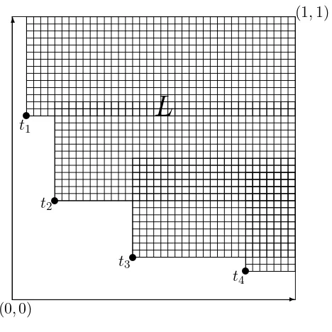
Figure 2: An upper layer L=∪4 1Eti
Lemma 4.3. If T satisfies Assumption 2.4 and s, t∈T, then dH(As, At), dH(Es, Et)≤d(s, t).
Proof. Let ǫ=d(s, t). Since both As, At ⊆As∨t, it is enough to show that As∨t ⊆Aǫs (and so
by symmetry,As∨t⊆Atǫ) . Ifu∈As∨t, then by Assumption 2.4
d(u, u∧s) = d(u∧(s∨t),(u∧s)∧(s∨t)) = d(((u∧s)∨(u∧t)),(u∧s))
≤ d(u∧s, u∧t)
≤ d(s, t) =ǫ,
and if follows that u∈Aǫs, as required.
The proof fordH(Es, Et) is similar. ✷
We now introduce the space U of upper layers:
Definition 4.4. A nonempty closed set B ⊆ T is called an upper layer if t ∈ B ⇔ Et ⊆ B.
The collection of upper layers is denoted by U.
The shaded region in Figure 2 illustrates an upper layerL. Note that L=∪t∈LEt=∪4i=1Eti.
Lemma 4.5. If(T, d) is a complete separable metric space satisfying Assumptions 2.1-2.4, then (U, dH) is a complete separable metric space satisfying Assumptions 2.1, 2.2 and 2.3 under the
partial order of reverse set inclusion: i.e. L1 ≤L2 ⇔L1 ⊇L2, ∀L1, L2,∈ U.
Proof. The spaceU is closed under arbitrary intersections (sups) and finite unions (infs). There-fore, since E1 = {1} and E0 = T, U has both a maximum and minimum, and is therefore a
τ1
To show that (U, dH) satisfies Assumption 2.3 (and is therefore separable), we define Un to be
the (finite) lattice of upper layers generated by the sets Et, t∈Tn: i.e. L∈ Un if and only ifL
is a (finite) union of setsEt, t∈Tn. Sincet′ < t < t′′ ⇒Et′ ⊃Et ⊃Et′′, Assumption 2.3 is an
immediate consequence of Assumption 2.4.3 and Lemma 4.3. For L∈ U, we have
L+n = ∪L′
Definition 4.6. Given a point process N on T, the induced random point measure N˜ on U
has (ordered) jumps at (ξk, k ≥1) for all k such that ξk is defined. In particular, for L ∈ U,
˜
N(AL)≥k if and only if ξk⊇L.
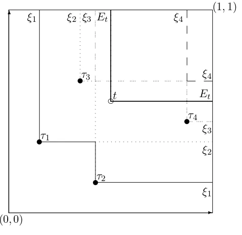
Figure 3 illustrates the embedding N → N˜ for a realization of a point process N with jump points τ1, ..., τ4. The lower boundaries of the adapted random sets ξi, i = 1, ..., are illustrated,
as is the lower boundary of the upper layer Et. We see that ˜N(AEt) = 2, since Et ⊂ ξ2 (i.e.
ξ2 ∈AEt), but Et6⊆ξ3 (i.e. ξ3 6∈AEt). This corresponds to the fact thatN(At) = 2.
Theorem 4.7. Let N be a strictly simple point process on a complete separable metric spaceT
that satisfies Assumptions 2.1-2.4. IfN˜ is defined as in Definition 4.6,
1. N˜ is a totally ordered strictly simple point process on(U,FU).
2. The law of N determines and is determined by the law of N˜.
According to the above theorem, we are able to construct a flow ˜f connecting any finite increasing
(in the partial order of reverse set inclusion) sequence (Lj)⊆ ∪nUn so that ˜N ˜ f
is a simple point
process on [0,1]. Denote any countable class of such flows by FN˜. For f ∈FN˜, the law of ˜N ˜ f
is uniquely determined by ΛN˜f˜, the compensator of ˜N
˜ f
with respect to its minimal filtration
FN˜f˜. This leads us to the following definition:
Definition 4.8. Let N be a strictly simple point process on T and N˜ its embedding in U. The
U-flow compensator Λ of N is the family of processes ˜
Λ :={ΛN˜f˜; ˜f ∈FN˜}
where FN˜ is a family of flows as defined above.
Our main result is now straightforward:
Theorem 4.9. Let N be a strictly simple point process on a complete separable metric space
T that satisfies Assumptions 2.1-2.4. The U-flow compensator of N exists and is unique. The law of N determines and is determined by its U-flow compensator Λ˜. In fact, the flows f˜used to determine the U-flow compensator may be restricted to the family of basic flows: f˜ is a basic flow if for each u ∈ [0,1], f(u) can be expressed as a finite union of the form f(u) =
∪k
i=1Eti, t1, ..., tk ∈T.
Proof. Lemma 4.5 and statement 1 of Theorem 4.7 permit us to apply Theorem 3.3 to ˜N: i.e. the law of ˜N determines and is determined by ˜Λ. In the proof of statement 1 of Theorem 4.7, it is seen that the basic flows inFN˜ suffice (cf. Lemma A.2). The result follows by statement 2
of Theorem 4.7. ✷
Comment 4.10. It is important to distinguish between flow and U-flow compensators. The flow compensator is defined by flows whose range is on the same space as the point process, while the U-flow compensator is defined by flows whose range is on a larger space. Therefore, theU-flow compensator ofN can be interpreted as the flow compensator of ˜N.
Comment 4.11. To conclude this section, we compare Theorems 3.3 and 4.9 in the case when
N is totally ordered. Iff ∈FN, then we may identify f with the basic flow ˜f on U such that
˜
f(u) = Ef(u) for all u ∈ [0,1]. Denote this class of flows by F−˜
N. From Lemma A.3 we have
that Nf(u) = ˜Nf˜(u) ∀u ∈ [0,1], and so Λ
Nf = Λ˜
Nf˜. Therefore, when N is totally ordered, the family of flows in Theorem 4.9 may be restricted to F−˜
N, and either the flow or theU-flow
(0,0)
(1,1)
ξ1
ξ2
ξ1
ξ4
ξ3
ξ2 ξ3 ξ4
t
t t
t
✻
✲
Figure 4: A single line process on [0,1]2
5
More examples
5.1 The single line process:
Asingle line process is a process whose jump points are all incomparable (see (8) for a detailed discussion). Such processes are strictly simple and theU-flow compensator can be reduced to the case of a single jump process. If N is a single line point process, it is completely characterized by the adapted random set ξ≡ξ1=∪τ∈∆NEτ, since the set of jump points, ∆N, is in fact the
set of theminimal points of ξ1 (see Figure 4):
∆N ={t∈ξ1 :6 ∃s∈ξ1\ {t} such thats≤t}.
The process M(t) =I{t ∈ξ} is not a point process on T, but the embedding ˜M inU defined by ˜M(L) =I{L⊆ξ}is a single jump point process onU with jump pointξ. ˜M will be referred to as the single jump process on U associated with the single line process N on T. Although
˜
M 6= ˜N, we do have the following:
Proposition 5.1. : The law of M˜ determines and is determined by the law of N.
Proof. Since ˜M is the first jump point of ˜N, its law is determined byN.
To prove the converse, we first show that the law of M (i.e. the finite dimensional distributions of M) is determined by that of ˜M, and then that the law of M determines that of N.
{Mt1 = 0, ..., Mtk = 0}=∩
k
i=1{ti ∈ξ}c = (∪ki=1{Eti ⊆ξ})
c, then
P(Mt1 = 0, ..., Mtk = 0) (9)
= 1−P(∪ki=1{Eti ⊆ξ})
= 1−
k
X
i=1
P(Eti ⊆ξ) + X
i<j
P(Eti∪Etj ⊆ξ) +...+ (−1)
kP(∪k
i=1Eti ⊆ξ),
which is equal to:
1−
k
X
i=1
P( ˜M(Eti) = 1) + X
i<j
P( ˜M(Eti∪Etj) = 1) +...
+(−1)kP( ˜M(∪ki=1Eti) = 1).
Observing that for anyk
P(Mt1 =...=Mtk−1 = 0, Mtk = 1)
= P(Mt1 =...=Mtk−1 = 0)−P(Mt1 =...=Mtk = 0)
and for anyj < k
P(Mt1 =...=Mtj = 0, Mtj+1 =...=Mtk = 1) = P(Mt1 =...=Mtj = 0, Mtj+2 =...=Mtk = 1)
−P(Mt1 =...=Mtj =Mtj+1 = 0, Mtj+2 =...=Mtk = 1),
it follows by induction that the finite dimensional distributions ofM can be reconstructed from probabilities of the form (9), and so are determined by the law of ˜M.
Now, it remains to show that the law ofNis determined by the law ofM. Clearly, in order to find terms of the formP(N(At1) =k1, ..., N(Atj) =kj), we can suppose that theti’s are dyadic. For any such event, we observe that all realizations of the point processN, forn(=n(ω)) sufficiently large, the sets Ct, t ∈ Tn will separate all the jump points and that the left-neighbourhoods
containing jump points will be incomparable (since the jump points are incomparable). Then
{N(At) =k} = ∪m∩n≥m{∃ exactlykincomparable left-neighbourhoods
Ct′ ∈ Cn withN(Ct′) = 1 and t′ ≤t}
= ∪m∩n≥m{∃ exactlykdyadics t′≤twithM(t′) = 1
and M(s) = 0,∀s < t′, s∈Tn}
Notice that the fact that the left-neighbourhoods of the jump points are incomparable is very important. Otherwise, there could exist s < t′ with N(Cs) = 1 and N(Ct′) = 1, in which
case Ms = 1 and Mt′ = 1. This cannot happen and so the left-neighbourhoods Ct′ with Mt′ = 1, Ms = 0,∀s < t′ are the only left-neighbourhoods with jump points. Then, we can
We have therefore reduced the problem of characterizing the law of a single line process N on
T to characterizing the law of a single jump process ˜M on U. This can be done by applying Example 3.5. We need to calculate G(L) =P(ξ ⊇L) for anyL in the range of a basic flow on
Proposition 5.2. Let N be a single line process onT andM˜ its associated single jump process on U. The flow compensator of the single jump processM˜ on U is defined as follows: for a basic flow f˜on U,
ΛM˜f˜(u) =−ln(1−G( ˜f(u∧τ
˜ f))
where Gis defined in (10). Conversely, the law of the point processN can be recovered from the flow compensator of M˜.
We remark here that the flow compensator of ˜M is defined onU, but is not theU-flow compen-sator ofN since ˜M 6= ˜N.
It should be noted that we have a generalization of Theorem 7.3.II in (3) which states that a simple point process N on a complete separable metric space is characterized by the values of its avoidance function P0(D) ≡P(N(D) = 0) for all D in a dissecting ring for the Borel sets.
Proposition 5.2 and (10) imply that ifN is a single line process, then its law is determined by the values ofP0 on sets of the form
D= (At1 ∪...∪Atk), t1, ..., tk dyadic and incomparable. (11)
There is a further simplification that can be made in the caseT = [0,1]2 whenN is a single line process satisfying a condition known in the literature as (F4):
(F4): Given t = (t1, t2) ∈ [0,1]2, the σ-fields F1(t) and F2(t) are conditionally independent
given FN(t), where
F1(t) = σ{N(u) : 0≤u1 ≤t1,0≤u2≤1}and
Lemma 5.3. LetN be a single line point process on[0,1]2 satisfying(F4). Then the values of the avoidance functionP0on sets of the form (11) are determined by the valuesP0(At) =P(N(At) =
0), t∈T. (These values will be referred to as one-dimensional avoidance probabilities.)
Proof. The proof is by induction onk. The casek= 1 is trivial and we assume that probabilities of the form
P(N(At1 ∪...∪Atk) = 0), t1, ..., tk dyadic and incomparable
are determined by one-dimensional avoidance probabilities if k ≤ n − 1. If points ti =
(ti,1, ti,2), i= 1, ..., n are incomparable, we may assume thatt1,1 < ... < tn,1 andt1,2 > ... > tn,2.
Let Bj := ∪ji=1Ati, j = 1, ..., n and A := A(tn−1,1,tn,2). From (F4), the random variables N(Bn−1\A) and N(Atn\A) are conditionally independent given theσ-algebra FN(A), and so
P(N(Bn) = 0)
= P(N(Bn−1\A) = 0, N(Atn \A) = 0, N(A) = 0)
= P(N(Bn−1\A) = 0, N(Atn \A) = 0|N(A) = 0)×P(N(A) = 0) = P(N(Bn−1\A) = 0|N(A) = 0)×P(N(Atn \A) = 0|N(A) = 0)
×P(N(A) = 0)
= P(N(Bn−1\A) = 0, N(A) = 0)×P(N(Atn\A) = 0, N(A) = 0)
÷P(N(A) = 0)
= P(N(Bn−1) = 0)P(N(Atn) = 0)
P(N(A) = 0) .
By the induction hypothesis, this is a function of one-dimensional avoidance probabilities of the
form P0(At) =P(N(At) = 0), t∈T. ✷
The preceding Lemma leads to an interesting corollary, which is an analogue of Theorems 3.1 and 3.3.
Corollary 5.4. Let N be a single line point process on [0,1]2 satisfying (F4). The law of
N determines and is determined by the laws of the family of the projected (single jump) point processes Nf, f ∈ FN. Consequently, the law of N determines and is determined by its flow
compensator Λ = (ΛNf :f ∈FN).
Proof. The law of Nf for any flow f passing through t will yield P(N(A
t) = 0). By Lemma
5.3, these probabilities determine the law ofN. ✷
We now see that the flow compensator Λ of N (on [0,1]2) characterizes the law of the point process in two extreme cases: the totally ordered point process (all jump points are comparable) and if (F4) is satisfied, the single line point process (all jump points are incomparable).
5.2 Renewal Processes:
here are that a renewal process is a strictly simple point process and its law is characterized by the law of N1, the single line process associated with ξ1. Consequently, we can apply the
characterization given in the preceding example to renewal processes.
Corollary 5.5. LetN be a renewal process on[0,1]2 satisfying (F4). The law ofN determines and is determined by the laws of the family of the projected point processes Nf,f ∈FN.
Conse-quently, the law ofN determines and is determined by its flow compensator Λ = (ΛNf :f ∈FN).
Proof. ΛNf characterizes the law of the first jump of Nf, which in turn is the only jump of
N1f. The result now follows from Corollary 5.4 and the fact that ifN is renewal, the law ofN1
determines the law of N. ✷
Comment 5.6. Since N(At) = 0⇔N1(At) = 0, Lemma 5.3 implies that the law of a renewal
processN satisfying (F4) is determined by its one-dimensional avoidance probabilitiesP0(At) =
P(N(At) = 0), t∈T.
5.3 The Homogeneous Poisson Process:
Corollary 5.5 leads to a new characterization of the two-parameter homogeneous Poisson process. Indeed, the minimal filtration of any Poisson process satisfies (F4) and it is proven in (8) that the two-parameter homogeneous Poisson process is renewal. Therefore, we have the following:
Theorem 5.7. A strictly simple point process on [0,1]2 is a homogeneous Poisson process with intensity c (c is a positive constant) if and only if it is renewal, (F4) is satisfied, and its flow compensator Λ is deterministic withΛNf(u) =cλ(Af(u)) ∀u∈T (λdenotes Lebesgue measure).
Proof. If N is a homogeneous Poisson process with intensity c, then Nf is Poisson with mean measure ΛNf. This and the discussion preceding the theorem prove the “only if” statement. Conversely, since N is renewal and (F4) is satisfied, as in Corollary 5.5 the law of N1 is
determined by Λf, and this in turn determines the law of N. For any homogeneous Poisson
process Np with intensity c, the law of N1p must equal that ofN1 (this follows from “only if”).
Since bothNpandN are renewal, their distributions are equal. This completes the proof of “if”.✷
Since ΛNf is deterministic, this means that the projection Nf is a Poisson process along each flow.
It is interesting to compare this characterization to the characterization given by G. Aletti and V. Capasso in (1): A strictly simple point process on [0,1]2 is a homogeneous Poisson process if and only if (F4) is satisfied and for each flow f, the projection Nf has the deterministic
compensator ΛNf (as defined above) with respect to the filtration Gf = (Gf(u),0 ≤ u ≤ 1) where Gf(u) = FN(f(u)). As observed in Section 3, the filtration Gf is strictly larger than
FNf and the fact that Nf is Poisson does not immediately imply that its compensator will
be deterministic with respect to a filtration larger than its minimal filtration FNf
5.4 A comparison of histories:
As a final general example, ifN is a strictly simple point process onT = [0,1]2 we would like to compare the “history” associated with the family ˜Λ of theU-flow compensator with the histories associated with Λwand Λ∗(see (11) for more details). First we recall that Λw is the compensator associated with the strict past
FN ={FN(t) :t∈T}= (σ{N(As) :s∈At}:t∈T),
while Λ∗ is associated with the strong past
FN∗ ={FN∗(t) :t∈T}= (σ{N(As) :s∈Dt=Etc}:t∈T).
For any flow ˜f ∈FN˜, we have
FN˜
˜ f
={FN˜
˜ f
(u) : 0≤u≤1}= (σ{N˜f˜(v) : 0≤v≤u}: 0≤u≤1),
and for t∈T, let
FFN˜(t) =σ(FN˜ ˜ f
(u) : ˜f ∈FN˜, u= ˜f
−1
(Et)).
FFN˜(t) may be regarded as the information associated with all the projections ˜N
˜ f
up to time ˜
f−1(Et) for flows ˜f ∈FN˜ passing through Et. It may be seen that FN(t) ⊂ FFN˜(t)⊂ FN ∗
(t). As an illustration, refer to Figure 3: t is an arbitrary point of the plane, τ1, τ2, τ3 and τ4 are
the jump points of a given realization of the point process N and ξ1, ..., ξ4 are the associated
adapted random sets. Note that ξ1, ξ2 ⊇Et, and so the family of flows through Et will allow
us to trace back the locations ofτ1, τ2 and τ3. However, since ξ3 6⊆Et,FFN˜(t) will contain no information about ξ3 or ξ4, and so τ4 will not be captured. Consequently, the jump points τ1
and τ2 are captured by all three σ-algebras. Point τ4 is only captured by FN
∗
(t); the “strict past”FN(t) of t does not capture τ4 because τ4 is not smaller than t and, as just noted, the
location ofτ4 cannot be reconstructed fromFFN˜(t) either. Finally, pointτ3 is captured by both
FN∗(t) and FFN˜(t), but obviously not by FN(t).
More generally, FFN˜(t) allows us to reconstruct all the sets ξ
k such that ξk ⊇ Et but contains
no information about ξk if ξk 6⊇ Et. Therefore, FFN˜(t) identifies all jump points τ such that
N(Aτ) ≤ N(At) (but no others). All of these jump points are contained in Dt and so are
captured by FN∗(t) (which may contain information about other jump points), but are not necessarily contained inAtand so may not be captured by FN(t). Therefore,
FN(t)⊂ FFN˜(t)⊂ FN∗(t).
A
Appendix: Proofs of Theorems 3.1 and 4.7
Proof of Theorem 3.1
In what follows, we prove that the finite dimensional distributions ofN on the sets inCn can be
reconstructed from the laws ofNf, f ∈F N.
To avoid multiple subscripts and superscripts, we fix nand letTn= (t0=0, t1, ..., tm =1) and
denote Aj =Atj and Cj =C
n
tj.Recall that Ci and Cj are incomparable if and only if ti and tj are incomparable and thatN(C0) =N({0}) = 0. Using the laws ofNf, f ∈F we must be able
to construct
P(N(C1) =k1, ..., N(Cm) =km). (12)
Ifki >0 and kh >0 for Ci, Ch incomparable, the probability in (12) is 0. Thus, we can assume
without loss of generality thatki6= 0 if and only ifi∈ {i1, ...ih}=:Hwhereti1 < ti2 < ... < tih. We can make a few simplifications. First, we observe that
{N(Ci) = 0 ∀Ci⊆T\Aih}={N(T \Aih) = 0}. (13)
Next, note that any flowf connecting (ti1, ti2, ..., tih) can be reparameterized and extended to connect (ti1, ti2, ..., tih,1). Iff(u) =tih,f(1) =1 thenN
f(1)−Nf(u) =N(T \A
ih). It follows that if the finite dimensional distributions of (N(Ci) :Ci ⊆Aih) can be determined byN
f for
flows f connecting (ti1, ti2, ...tih), then by (13), the probabilities in (12) can be determined by extending these flows to1. Therefore, we need only consider the finite dimensional distributions of (N(Ci) : Ci ⊆ Aih) and so to avoid changing notation, we will now assume without loss of generality that in (12) the setsC1, ..., Cm are the left neighbourhoods ofCn contained inAih. Let H′ denote the set of all i 6∈ H such that ti ∈ Aih and ti is comparable with tℓ for every
ℓ∈H:
H′ = {i:ti < tih and ∀ℓ∈H, eitherti < tℓ orti> tℓ} = {i:ti < ti1 or∃ℓ,2≤ℓ≤hsuch that tiℓ−1 < ti < tiℓ}.
Next, let
H′′={i:ti< tih, i6∈H
′∪H}.
We note here that if ℓ ∈ H′′, then there exists i ∈ H such that Cℓ and Ci are incomparable.
Therefore, if N(Ci)>0 ∀i∈H, it automatically follows thatN(Cℓ) = 0 ∀ℓ∈H′′. Now we see
that ifki>0 if and only ifi∈H,
P(N(C1) =k1, ...N(Cm) =km)
= P(∩i∈H{N(Ci) =ki} ∩j∈H′ {N(Cj) = 0} ∩
ℓ∈H′′ {N(Cℓ) = 0}) (14)
= P(∩i∈H{N(Ci) =ki} ∩j∈H′ {N(Cj) = 0}). (15)
The equality of (14) and (15) follows from the fact that ifℓ∈H′′, then necessarilyN(Cℓ) = 0.
We proceed by induction on|H′|:=the cardinality ofH′. In what follows, keep in mind that|H′|
is the number of left neighbourhoodsC ∈ Cnsuch thatC⊆Aih,N(C) = 0 andC is comparable withall of the left neighbourhoodsC′ ⊆Aih,C
′ ∈ C
If|H′|= 0, then forij ∈H (and definingAi0 =∅),Aij\Aij−1 =Cij∪ ∪ℓ∈H′′,tℓ∈Aij\Aij−1Cℓ and sinceN(Cℓ) = 0 necessarily forℓ∈H′′,
(12) = (15) =P(∩i∈H{N(Ci) =ki}) =P(∩hj=1{N(Aij\Aij−1) =kij}). (16)
The probability in (16) is determined by the finite dimensional distributions of Nf for any flow
f ∈F connecting (ti1, ...tih): if f(uj) =tij, j= 1, ..., h,
P(∩hj=1{N(Aij\Aij−1) =kij}) =P(∩
h
j=1{Nf(uj)−Nf(uj−1) =kij}).
Proceeding inductively, we assume that any probabilities of the form in (15) can be determined by the laws ofNf forf ∈Fnwhenever|H′| ≤ℓ−1. (This assumption is made forarbitrary Aih, and correspondingH′.) Assume that |H′|=ℓ. There exists 1≤j ≤h such that{t
i:i∈H′} ⊆Aij but{ti:i∈H′} 6⊆Aij−1.
Since {ti :i ∈ H′} ⊆Aij, it follows that for j < k ≤h, ifN(Cik) > 0 then N(Aik \Aik−1) = N(Cik) and (as in (16)), probabilities of the form
P(∩hr=j+1{N(Cir) =kir} ∩q∈H′′,tq<tih,tq6≤tij {N(Cq) = 0})
are determined by the laws of Nf for flows f connecting (tij, ..., tih). If it can be shown that probabilities of the form (assumingkir >0 for r= 1, ..., j)
P(∩1≤r≤j{N(Cir) =kir} ∩j∈H′ {N(Cj) = 0} ∩q∈H′′,tq<t
ij {N(Cq) = 0})
=P(∩1≤r≤j{N(Cir) =kir} ∩j∈H′ {N(Cj) = 0}) (17)
can be determined by the laws ofNf for flowsf connecting (t0, t1, ..., tij−1, tij), then flows from the two families can be joined at tij to yield a single family of flows F
′ ⊆F such that (15) is determined by the laws of {Nf :f ∈F′}.
Therefore, the final step in the proof is to show that probabilities of the form (17) can be determined by the laws of Nf for flowsf ∈F connecting (t
0, t1, ..., tij−1, tij). By the induction hypothesis, such flows will determine the following probabilities:
P(∩1≤r≤j−1{N(Cir) =kir} ∩q∈H′,tq<tij
−1 {N(Cq) = 0}
∩{N(Aij\Aij−1) =kij}) (18) where we must havekir >0, i= 1, ..., j−1, but kij can take on any value. We note that since
kij−1 >0,N(Cv) = 0 iftv ∈Aij \Aij−1 and tv 6> tij−1. Therefore,
N(Aij \Aij−1) =N(Cij) +
X
v∈H′:t
ij−1<tv<tij
N(Cv). (19)
Consider probabilities of the form
P(∩jr=1{N(Cir) =kir} ∩ ∩v∈H′,tij
−1<tv<tij{N(Cv) =kv}
∩q∈H′
,tq<tij−1{N(Cq) = 0}). (20) where kir > 0, i = 1, ..., j −1 and kv > 0 for at least one v ∈ H
′
• kij > 0 and there exist r ≥ 1 and v1, ...vr ∈ H
To summarize, we have shown that the probability in (20) is completely determined by the laws of Nf for f ∈F in the family of flows connecting (t0, t1, ..., tij−1, tij) provided that kir > 0, r = 1, ..., j −1 and kv > 0 for at least one v ∈ H
′
, tij−1 < tv < tij. In particular, if
kir > 0, r = 1, ..., j−1 andk > 0, the laws of N
f for f ∈ F in the family of flows connecting
(t0, t1, ..., tij−1, tij) determine
>From (22) we see that the probabilities in (23) are determined by the laws ofNf forf ∈F in the family of flows connecting (t0, t1, ..., tij−1, tij). This completes the proof. ✷
Proof of Theorem 4.7:
The proof will proceed in a series of Lemmas. First, we must verify that in fact ˜N is a totally ordered point process on U; i.e. a measurable mapping from (Ω,F) to the space of counting measures on (U,FU), where FU is the Borel σ-field generated by dH, that N({L}) = 0 or 1,
Lemma A.1. If N is a strictly simple point process on T, then N˜ is a totally ordered point process on (U,FU).
Proof. By Proposition 7.1.VIII of (3), ˜N is a point measure if it can be shown that ˜N(U) is a random variable for all U in a semiring of bounded Borel sets in U generating FU. (Keep in mind that U is a set of sets.) By the proof of the preceding Lemma, it is easily seen that the class of left-neighbourhoods associated with Unforn≥1 form such a semiring.
Next, for any left-neighbourhood U associated with Un, ˜N(U) can be expressed as a linear
combination of random elements of the form ˜N(AL) for some L ∈ Un, so it suffices to show
that ˜N(AL) is a random variable. Since ∪nTn is dense in T, measurability follows from the
representation in (24) below:
{N˜(AL)≥k} = {ξk⊇L}
= {L⊆ ∪τ1,...τk∈∆NEτ1∨...∨τk}
= ∩n∩t∈Tn,t∈L{N(At)≥k}. (24)
˜
N is an integer-valued measure putting mass 1 on ξ1, ξ2, ..., and by definition, we have
ξ1 ≤ξ2 ≤...(in the partial order of reverse set-inclusion). That ˜N is simple follows from that
fact thatN is strictly simple. First, no jump point in ∆N can be the sup of other jump points, since if τk = ∨k1−1τi where τk−1 6= ∨1k−2τi, then any flow f connecting (∨1k−2τi)+n with (τk)+n
would have a projection Nf with a double jump at u, where u = inf{v : f(v) ≥ τ
k}. Since
s6=t⇔Es6=Et, it follows thatξk−1 6=ξk. ⋄
To complete the proof of the first statement of Theorem 4.7, we must prove that the embedded process ˜N is strictly simple.
Lemma A.2. If N is strictly simple, then so is N˜. FN˜ can be restricted to the class of basic flows on U.
Proof. It is enough to show that for L0 =T ⊃L1 ⊃ ...⊃ Lm ={1} ∈ Un there exists a flow
˜
f : [0,1]→ U with ˜f(mk) =Lk, k= 0, ..., m such that ˜N ˜ f
is simple. Without loss of generality, we may assume that for 0 ≤ j ≤ m, Lj = ∪mi=jEti where Tn = (t0 = 0, t1, ..., tm = 1) is a
consistent ordering of the elements of Tn: i.e. ti> tj ⇒i > j.
To construct the flow ˜f, for each 0≤j ≤m−1, choose tj+ ∈ {tj+1, ..., tm} such thattj+ > tj
and there exist no other pointsth ∈ {tj+1, ..., tm} with tj < th < tj+. Note that t(m−1)+ = 1
since the ordering is consistent. SinceN is strictly simple, for 0 ≤ j ≤ m−1 we may choose a flowfj connecting tj and tj+ such that (with an appropriate reparametrization) fj(mj ) =tj,
fj(j+1m ) = tj+ and Nfj(u) is simple for u ∈ (mj ,j+1m ]. Now define ˜f(0) := E0 = T and for u∈(mj,j+1m ],
˜
f(u) :=Efj(u)∪ ∪
m
h=j+1Eth. (25)
To see that ˜f is a flow on U, we first observe that ˜f is strictly increasing since fj is and so j
m < u < v≤ j+1
m ⇒fj(u)< fj(v)⇒ Efj(u) ⊃Efj(v); by the choice of tj+,Efj(u) 6⊆ ∪
m
definition of tj+ and continuity offj, ˜f(ur) →dH ∪
Therefore, we are able to construct a basic flow ˜f connecting any increasing (in the partial
order of reverse set inclusion) sequence (Lj)⊆ ∪nUn so that ˜N ˜ f
is simple. By definition, ˜N is strictly simple and we can restrictFN˜ to the class of basic flows. ⋄
To prove the second statement in Theorem 4.7, we show thatN and ˜N are dual: each determines the law of the other. First, we need the following:
Lemma A.3. For t∈T, N(At) =k if and only if N˜(AEt) =k.
Lemma A.4. The law of N determines and is determined by the law ofN˜.
Proof. Since the laws of N and ˜N are determined by the finite dimensional distributions on the left-neighbourhoods generated by Tn and Un respectively, for n ≥ 1 (cf. (3). Proposition
6.2.III), by additivity it is enough to consider the finite dimensional distributions of the form
P(N(At1) =k1, ..., N(Atj) =kj) andP( ˜N(AL1)≥k1, ...,N˜(ALj)≥kj).
>From Lemma A.3, we have that fort1, ..., tj ∈T
P(N(At1) =k1, ..., N(Atj) =kj) =P( ˜N(AEt1) =k1, ...,N˜(AEtj) =kj),
and so the law of ˜N determines that of N. Conversely, since Tn is finite, (24) implies that the
law ofN determines that of ˜N:
B
Appendix: Renewal Processes
Here we define renewal processes on [0,1]2, adapting the definition given in (8) to the notation used in this paper. We refer the reader to (8) for details.
Definition B.1. For an arbitrary Borel set B⊆[0,1]2, the set of minimal points of B is min(B) :={t∈B :s6≤t, ∀s∈B such that s6=t}.
Definition B.2. Let N be a strictly simple point process on [0,1]2. With ξ
n defined as in (8),
denote:
• ∆N :={τ :N({τ}) = 1}. This is the set of jump points of the processN.
• ε(ξn) is the finite set of minimal points ofξn, and letεN :=∪∞n=1ε(ξn). The points inε(ξn)
will be denoted by {τj(n), j = 1, ...,}; the numbering τ1(n), τ2(n)... may be defined arbitrarily.
• ξn+:=∪k6=j(Eτ(n) k
∩Eτ(n) j
). If ξn has only one minimal point, then ξn+:=∅.
Comments B.3.
1. In general, ∆N ⊆εN and εN is the closure of ∆N under suprema; both sets are finite. If
τ ∈ ∆N and N(Aτ) = i, then τ = τj(i) for some j. Conversely, while all of the minimal
points ofξ1 are in ∆N (in fact, ε(ξ1) = min(∆N)), ifi > 1,τj(i) is not necessarily a jump
point ofN but will always be the supremum of ijump points.
2. The random sets ξn are determined by ε(ξn) and vice versa. Likewise, ξ+n is determined
by ε(ξn); each of its minimal points is the sup of a pair of minimal points of ξn, and the
setξn\ξ+n is the disjoint union of the mutually incomparable sets Eτ(n) j
\ξ+
n, j= 1,2, ...
3. By definition, N(At) ≥ i+ 1 if t ∈ ξi+, and so ξi ⊆ ξi+1 ⊆ ξi+, ∀i. The set of minimal
points ofξi+1 consists of the minimal points of ξi+ as well as the minimal jump points of
N contained in the set ξi\ξi+: i.e.
ε(ξi+1) = ε(ξi+)∪min(∆N∩(ξi\ξi+))
= ε(ξi+)∪ ∪jmin(∆N ∩(Eτ(i) j \
ξi+)). (26)
The representation in (26) motivates the following definition of the renewal property.
Definition B.4. Let N be a (strictly simple) point process on [0,1]2 with associated adapted random sets ξi, i≥1, and let τ1(i), τ
(i)
2 , .... denote the minimal points ofξi. Let N1 be the single
line process with jump points ε(ξ1). N is a renewal point process if for every i≥1,
• Given ξi, the process N behaves independently on each of the disjoint incomparable sets
E
τj(i) \ξ +
i , j= 1,2, ... .
• Givenξi, the law ofmin(∆N∩(Eτ(i) j
\ξ+i ))is the same as the law of ((∆M⊕τj(i))∩(Eτ(i) j
\
ξi+)), where M is an independent copy ofN1, and (∆M⊕τj(i)) is the set of jump points of
We see that the law of ξi+1 given ξi does not depend on i, and is determined by the law of
min(∆N ∩(Eτ(i) j
\ ξ+i )); this in turn is determined by the law of N1. Therefore, the law of
the renewal process N is completely characterized by the law of N1. See (8) for a rigorous
development.
References
[1] Aletti, G., and Capasso, V., Characterization of spatial Poisson along optional increas-ing paths, a problem of dimension’s reduction, Stat. Probab. Letters 43, 343-347 (1999). MR1707943
[2] Andersen, P.K., Borgan, O., Gill, R.D. and Keiding, N.Statistical Models Based on Count-ing Processes, Springer-Verlag, 1993. MR1198884
[3] Daley, D.J., and Vere-Jones, D.,An Introduction to the Theory of Point Processes, Springer-Verlag, 1988. MR0950166
[4] Gierz, G., Hofmann, K.H., Keimel, K., Lawson, J.D., Mislove, M. and Scott, D.S.,A Com-pendium of Continuous Lattices, Springer-Verlag, 1980. MR0614752
[5] Ivanoff, B.G. and Merzbach, E., Characterizations of compensators for point processes on the plane,Stochastics and Stoch. Rep.29, 395-405 (1990). MR1042067
[6] Ivanoff, B.G. and Merzbach, E., Set-indexed Martingales, Monographs on Statistics and Applied Probability, 85, Chapman & Hall/CRC, 2000. MR1733295
[7] Ivanoff, B.G. and Merzbach, E., Random censoring in set-indexed survival analysis. Ann. Appl. Probab.12, 944-971 (2002). MR1925447
[8] Ivanoff, B.G. and Merzbach, E., What is a multi-parameter renewal process?, Stochastics, 78, 411-441 (2006).
[9] Jacod, J., Multivariate point processes: Predictable projection, Radon-Nikodym deriva-tives, representation of martingales, Z. Wahr. verw. Gebiete 31, 235-253 (1974/75). MR0380978
[10] Mazziotto, G., and Merzbach, E., Point processes indexed by directed sets, Stoch. Proc. Applic.30, 105-119 (1988). MR0968168
![Figure 4: A single line process on [0, 1]2](https://thumb-ap.123doks.com/thumbv2/123dok/976482.914960/16.595.189.424.132.356/figure-single-line-process-on.webp)
