www.elsevier.nlrlocaterisprsjprs
A robust linear least-squares estimation of camera exterior
orientation using multiple geometric features
Qiang Ji
a,), Mauro S. Costa
b, Robert M. Haralick
b, Linda G. Shapiro
ba
Department of Computer Science, UniÕersity of NeÕada at Reno, Reno, NV 89557, USA
b
Department of Electrical Engineering, UniÕersity of Washington Seattle, WA 98195, USA
Abstract
Ž .
For photogrammetric applications, solutions to camera exterior orientation problem can be classified into linear direct and non-linear. Direct solutions are important because of their computational efficiency. Existing linear solutions suffer from lack of robustness and accuracy partially due to the fact that the majority of the methods utilize only one type of geometric entity and their frameworks do not allow simultaneous use of different types of features. Furthermore, the orthonormality constraints are weakly enforced or not enforced at all. We have developed a new analytic linear least-squares framework for determining camera exterior orientation from the simultaneous use of multiple types of geometric features. The technique
utilizes 2Dr3D correspondences between points, lines, and ellipse–circle pairs. The redundancy provided by different
geometric features improves the robustness and accuracy of the least-squares solution. A novel way of approximately imposing orthonormality constraints on the sought rotation matrix within the linear framework is presented. Results from experimental evaluation of the new technique using both synthetic data and real images reveal its improved robustness and
accuracy over existing direct methods.q2000 Elsevier Science B.V. All rights reserved.
Keywords: exterior orientation; linear methods; least-squares; orthonormality constraints; feature fusion
1. Introduction
Camera exterior orientation estimation is an es-sential step for many photogrammetric applications. It addresses the issue of determining the exterior
Ž .
parameters position and orientation of a camera with respect to a world coordinate frame. Solutions to the exterior orientation problem can be classified
)Corresponding author. Tel.:
q1-775-784-4613; fax:q 1-775-784-1877.
Ž .
E-mail address: [email protected] Q. Ji .
into linear and non-linear methods. Linear methods have the advantage of computational efficiency, but they suffer from lack of accuracy and robustness. Non-linear methods, on the other hand, offer a more accurate and robust solution. They are, however, computationally intensive and require initial esti-mates. The classical non-linear photogrammetric
ap-Ž
proach to exterior orientation e.g. the bundle adjust-.
ment method requires setting up a non-linear least-squares system. Given initial estimates of the exte-rior parameters, the system is then linearized and solved iteratively. While the classical technique guarantees the orthonormality of the rotation matrix and delivers the best answer, it, however, requires
0924-2716r00r$ - see front matterq2000 Elsevier Science B.V. All rights reserved.
Ž .
good initial estimates. It is a well-known fact that the initial estimates must be close or the system may not converge quickly or correctly. Hence, the quality of initial estimates is critical since it determines the convergence speed and the correctness of the itera-tive procedure. Robust and accurate linear solutions, which are often used to provide initial guesses for non-linear procedures, are therefore important for photogrammetric problems.
Numerous methods have been proposed to analyt-ically obtain camera exterior parameters. Previous methods have primarily been focused on using sets of 2D–3D point correspondences to solve for the transformation matrix, followed by extracting the camera parameters from the solved transformation. The linear method using points is well known in photogrammetry as direct linear transformation (DLT .)
The original proposal of DLT method appears in Ž .
Abdel-Aziz and Karara 1971 . Since then, different variations of DLT methods have been introduced.
Ž .
For example, Bopp and Krauss 1978 published a variation of the DLT, incorporating added constraints
Ž .
into the solution. Okamoto 1981 gave an alterna-tive derivation of the DLT from a more general
Ž .
mathematical framework. Shan 1996 introduced a linear solution for object reconstruction from a stere-opair without interior orientation and less require-ments on known points than the original DLT formu-lation.
In computer vision, the DLT-like methods include
Ž .
the three-point solution Fischler and Bolles, 1981 , Ž
the four-point solutions Hung et al., 1985; Holt and .
Netravali, 1991 , and the six- or more-point solutions ŽSutherland, 1974; Tsai, 1987; Faugeras, 1993 . Har-.
Ž .
alick et al. 1994 reviewed and compared major direct solutions of exterior orientation using three-point correspondences and characterized their perfor-mance under varying noisy conditions. Sutherland Ž1974 provided a closed-form least-squares solution. using six or more points. The solution, however, is
Ž .
only up to a scale factor. Faugeras 1993 proposed a similar technique that solves the scale factor by applying a normality constraint. His solution also includes a post-orthogonalization process that en-sures the orthonormality of the resulting rotation
Ž .
matrix. Tsai 1987 presented a direct solution by decoupling the camera parameters into two groups;
each group is solved for separately in different stages. While efficient, Tsai’s method does not impose any of the orthonormal constraints on the estimated rota-tion matrix. Also, the errors with the camera parame-ters estimated in the earlier stage can significantly affect the accuracy of parameters estimated in the later stage.
These methods are effective and simple to imple-ment. However, they are not robust and are very
Ž
susceptible to noise in image coordinates Wang and .
Xu, 1996 , especially when the number of control points approaches the minimum required. For the
Ž . three-point solutions, Haralick et al. 1994 show that even the order of algebraic substitutions can render the output useless. Furthermore, the point distribution and noise in the point coordinates can also dramatically change the relative output errors. For least-squares-based methods, a different study by
Ž .
Haralick et al. 1989 show that when the noise level exceeds certain level or the number of points is below certain level, these methods become extremely unstable and the errors skyrocket. The use of more points can help relieve this problem. However, gen-eration of more control points often proves to be difficult, expensive, and time-consuming. Another disadvantage of point-based methods is the difficulty with point matching, i.e., finding the correspon-dences between the 3D scene points and 2D image pixels.
In view of these issues, other researchers have investigated the use of higher-level geometric fea-tures such as lines or curves as observed geometric entities to improve the robustness and accuracy of linear methods for estimating exterior parameters. Over the years, various algorithms using features other than points for exterior orientation problems have been introduced both in photogrammetry and
Ž
computer vision Doehler, 1975; Haralick and Chu, 1984; Paderes et al., 1984; Mulawa, 1989; Mulawa and Mikhail, 1988; Tommaselli and Lugnani, 1988; Chen and Tsai, 1990, 1991; Echigo, 1990; Lee et al., 1990; Liu et al., 1990; Wang and Tsai, 1990; Fin-sterwalder, 1991; Heikkila, 1991; Rothwell et al., 1992; Weng et al., 1992; Mikhail, 1993; Petsa and
. Ž .
Szczepan-Ž .
ski 1958 reviewed nearly 60 different solutions for space resection, dating back to 1829, for the simulta-neous and separate determination of the position and rotation parameters. An iterative Kalman filtering method for space resection using straight-line fea-Ž . tures was described in Tommaselli and Tozzi 1996 .
Ž .
Masry 1981 described a method for camera abso-Ž .
lute orientation and Lugnani 1980 for camera exte-rior orientation by spatial resection, using linear
Ž .
features. Drewniok and Rohr 1997 presented an approach for automatic exterior orientation of aerial imagery that is based on detection and localisation of
Ž . Ž .
planar objects manhole covers . Ethrog 1984 used parallel and perpendicular lines of objects for estima-tion of the rotaestima-tion and interior orientaestima-tion of non-metric cameras.
Researchers have also used other known geomet-ric shapes in the scene to constrain the solution. Such
Ž .
shapes can be 2D straight lines, circles, etc. or 3D Žfeatures on a plane, cylinder, etc.. ŽMikhail and
. Ž
Mulawa, 1985 . Others Kruck, 1984; Kager, 1989; .
Forkert, 1996 have incorporated geometric con-straints such as coordinate differences, horizontal and space distances, and angles to improve the tradi-Ž . tional bundle adjustment method. Heikkila 1990 ,
Ž . Ž .
Pettersen 1992 , and Maas 1999 employed a
mov-Ž .
ing reference bar known distance for camera orien-tation and calibration.
Ž . In computer vision, Haralick and Chu 1984 presented a method that solves the camera exterior parameters from the conic curves. Given the shape of conic curves, the method first solves for the three rotation parameters using an iterative procedure. The three translation parameters are then solved analyti-cally. The advantage of this method is that it does not need to know the location of the curves and it is more robust than any analytical method in that rota-tion parameter errors are reduced to minimum before they are used analytically to compute translation Ž . parameters. In their analytic method, Liu et al. 1990
Ž .
and Chen and Tsai 1990 discussed direct solutions for determining camera exterior parameters based on a set of 2D–3D line correspondences. The key to their approach lies in the linear constraint they used. This constraint uses the fact that a 3D line and its image line lie on the same plane determined by the center of perspectivity and the image line. Rothwell
Ž .
et al. 1992 discussed a direct method that
deter-mines camera parameters using a pair of conic curves. The method works by extracting four or eight points from conic intersections and tangencies. Exterior camera parameters are then recovered from these
Ž .
points. Kumar and Hanson 1989 described a robust technique for finding camera parameters using lines.
Ž .
Kamgar-Parsi and Eas 1990 introduced a camera calibration method with small relative angles. Gao Ž1992 introduced a method for estimating exterior. parameters using parallelepipeds. Forsyth et al. Ž1991 proposed to use a pair of known conics or a. single known circle for determining the pose of the
Ž .
object plane. Haralick 1988 and Haralick and Chu Ž1984. presented methods for solving for camera parameters using rectangles and triangles. Abidi Ž1995 presented a closed form solution for pose. estimation using quadrangular targets. Linnainmaa
Ž .
and Harwood 1988 discussed an approach for de-termination of 3D object using triangle pairs. Chen
Ž .
and Tsai 1991 proposed closed solution for pose estimation from line-to-plane correspondences and studied the condition of the existence of the closed
Ž .
solution. Ma 1993 introduced a technique for pose estimation from the correspondence of 2Dr3D con-ics. The technique, however, is iterative and requires a pair of conics in both 2D and 3D.
im-proves the robustness and accuracy of the least-squares solution, therefore improving the precision of the estimated parameters. To our knowledge, no previous research attempts have been made in devel-oping a linear solution to exterior orientation with simultaneous use of all three classes of features.
Ž .
Work by Phong et al. 1995 described a technique in which information from both points and lines is used to compute the exterior orientation. However, the method is iterative and involves only points and lines.
Another major factor that contributes to the lack of robustness of the existing linear methods is that orthonormality constraints on the rotation matrix are often weakly enforced or not enforced at all. In this research, we introduce a simple, yet effective, scheme for approximately imposing the orthonormal con-straints on the rotation matrix. While the scheme does not guarantee that the resultant rotation matrix completely satisfies the orthonormal constraints, it does yield a matrix that is closer to orthonormality than those obtained with competing methods.
This paper is organized as follows. Section 2 briefly summarizes the perspective projection geom-etry and equations. Least-squares frameworks for estimating the camera transformation matrix from 2D–3D point, line, and ellipsercircle correspon-dences are presented in Sections 3–5, respectively. Section 6 discusses our technique for approximately imposing orthonormal constraints and presents the integrated linear technique for estimating the trans-formation matrix simultaneously using point, line, and ellipsercircle correspondences. Performance characterization and comparison of the developed integrated technique is covered in Section 7.
2. Perspective projection geometry
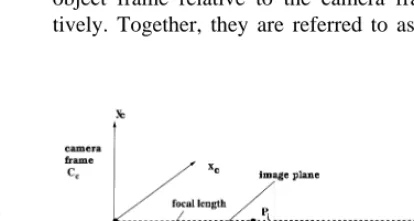
To set the stage for the subsequent discussion, this section briefly summarizes the pin–hole camera model and the perspective projection geometry.
Ž .t
Let P be a 3D point and x y z be the coordi-nates of P relative to the object coordinate frame C . Define the camera coordinate system C to haveo c
its z-axis parallel to the optical axis of the camera lens and its origin located at the perspective center.
Ž .t
Let xc yc zc be the coordinates of P in C .c
Define C to be the image coordinate system, with itsi
u-axis and Õ-axis parallel to the x- and y-axes of the camera coordinate frame, respectively. The origin of
[image:4.595.290.497.498.608.2]Ž .t C is located at the principal point. Let ui Õ be the coordinates of P , the image projection of P in C .i i
Fig. 1 depicts the pin–hole camera model.
Based on the perspective projection theory, the Ž .
projection that relates u,Õ on the image plane to
Ž .
the corresponding 3D point x , y , zc c c in the camera frame can be described by
x
u c
Õ
l
0
s0
ycŽ .
1f zc
where lis a scalar and f is the camera focal length.
Ž .t Ž .t
Further, x y z relates to xc y zc c by a rigid body coordinate transformation consisting of a rota-tion matrix and a translarota-tion. Let a 3=3 matrix R represent the rotation and a 3=1 vector T describe the translation, then
xc x
sR qT
Ž .
2yc
ž /
y0
zc zŽ where T and R can be parameterized as Ts tx ty
.t tz and
r11 r12 r13
Rs
r21 r22 r230
r31 r32 r33
R and T describe the orientation and location of the
object frame relative to the camera frame, respec-tively. Together, they are referred to as the camera
transformation matrix. Substituting the
parameter-Ž . ized T and R into Eq. 2 yields
t xc r11 r12 r13 x x
t
s q
Ž .
3yc r21 r22 r23
ž /
y y0
zc r31 r32 r330
z0
tzŽ .
Combining the projection Eq. 1 with the rigid Ž .
transformation of Eq. 2 and eliminating l yields the collinearity equations, which describe the ideal relationship between a point on the image plane and the corresponding point in the object frame
r x11 qr12yqr z13 qtx
usf
Ž .
4r31xqr32yqr33zqtz r21xqr22yqr23zqty Õsf
r31xqr32yqr33zqtz
For a rigid body transformation, the rotation ma-trix R must be orthonormal, that is, Rt
sRy1. The
constraint Rt
sRy1 amounts to the six
orthonormal-ity constraint equations on the elements of R
r2
qr2
qr2
s1 r r qr r qr r s0
11 12 13 11 21 12 22 13 23 2 2 2
r21qr22qr23s1 r r11 31qr r12 32qr r13 33s0
2 2 2
r31qr32qr33s1 r r21 31qr r22 32qr r23 33s0 5
Ž .
where the three constraints on the left column are referred to as the normality constraints and the three on the right column as the orthogonality constraints.
The normality constraints ensure that the row vectors of R are unit vectors, while the orthogonality con-straints guarantee orthogonality among row vectors.
3. Camera transformation matrix from point cor-respondences
Given the 3D object coordinates of a number of points and their corresponding 2D image coordi-nates, the coefficients of R and T can be solved for by a least-squares solution of an over-determined system of linear equations. Specifically, the least-squares method based on point correspondences can be formulated as follows.
Ž .
Let Xns x , y , z , nn n n s1, . . . , K, be the 3D coordinates of K points relative to the object frame
Ž .
and U s u , Õ be the observed image coordinates
n n n
of these points. We can then relate X and U vian n Ž .
the collinearity equations in Eq. 4 . Rewriting Eq. Ž .4 yields
fr x11 nqfr12ynqfr z13 nyu rn 31xnyu rn 32yn
yu rn 33znqftxyu tn zs0
Ž .
6 fr21xnqfr22ynqfr23znyu rn 31xnyÕn 32r ynyÕn 33r znqftyyu tn zs0
We can then set up a matrix M and a vector V as follows
fx1 fy1 fz1 0 0 0 yu x1 1 yu y1 1 yu z1 1 f 0 yu1
0 0 0 fx fy fz yÕ x yÕ y yÕ z 0 f yÕ
1 1 1 1 1 1 1 1 1 1
.
2 K=12 .
M s .
Ž .
7fxK fyK fzK 0 0 0 yu xK K yu yK K yu zK K f 0 yuK
0 0 0 fxK fyK fzK yu xK K yÕKyK yÕKzK 0 f yÕK0
t
12=1 r r r r r r r r r t t t
V s
ž
11 12 13 21 22 23 31 32 33 x y z/
Ž .
8where M is hereafter referred to as the collinearity matrix and V is the unknown vector of
To determine V, we can set up a least-squares problem that minimizes
2 5 52
j s MV
Ž .
9wherej2
is the sum of squared residual errors of all points. Given an overdetermined system, a least-squares solution to the above equation requires
mini-5 52
mization of MV . Its solution contains an arbi-trary scale factor due to the lack of constraints on R. To uniquely determine V, different methods have been proposed to solve for the scale factor. In the Ž . least-squares solution provided by Sutherland 1974 , the depth of the object is assumed to be unity; tzs1. Not only is this assumption unrealistic for most applications, but also the solution is constructed without regard to the orthonormal constraints that R
Ž .
must satisfy. Faugeras 1993 posed the problem as a constrained least-squares problem using a minimum
Ž of six points. The third normality constraint the last
. Ž .
one on the left column in Eq. 5 is imposed by Faugeras during the minimization to solve for the scale factor and to constrain the rotation matrix. The linearity in solution is preserved due to the use of a single normality constraint.
4. Camera transformation matrix from line corre-spondences
Given correspondences between a set of 3D lines and their observed 2D images, we can set up a system of linear equations that involve R, T, and the coefficients for 3D and 2D lines as follows. Let a 3D line L in the object frame be parametrically repre-sented as
L: XslNqP
Ž .t
where Xs x y z is a generic point on the line, l
is a scalar representing the signed distance from Ž .t
point P to point X, Ns A B C is the known
Ž .t
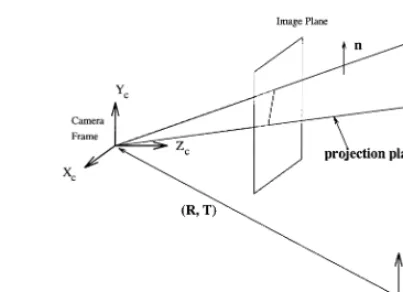
direction cosine vector and Ps Px Py Pz is a known point on the line relative to the object frame. Let the corresponding 2D line l on the image plane be represented by
[image:6.595.292.494.47.193.2]l : auqbÕqcs0
Fig. 2. Projection plane formed by a 2D image line l and the corresponding 3D line L.
Ideally, the 3D line must lie on the projection plane formed by the center of perspectivity and the 2D image line as shown in Fig. 2.
Relative to the camera frame, the equation of the projection plane can be derived from the 2D line equation as
afxcqbfycqczcs0
where f is the focal length. Since the 3D line lies on the projection plane, the plane normal must be per-pendicular to the line. Denote the plane normal by
t 2 2 2 2 2
Ž .
(
ns af, bf,c r a f qb f qc ; then given an ideal projection, we have
ntR N
s0
Ž
10.
Similarly, since point P is also located on the projection plane, this leads to
nt
Ž
R PqT.
s0Ž
11.
Ž . Ž .
Eqs. 10 and 11 are hereafter referred to as copla-narity equations. Equivalently, they can be rewritten as
A a r11qB a r12qC a r13qA b r21qB b r22
qC b r23qA c r31qB c r32qC c r33s0 P a rx 11qP a ry 12qP a rz 13qP b rx 21qP b ry 22
qP b rz 23qP c rx 31qP c ry 32qP c rz 33qa tx
Given a set of J line correspondences, we can set up a system of linear equations similar to those for
points that involve matrix H and vector V, where V is as defined before and H is defined as follows
A a1 1 B a1 1 C a1 1 A b1 1 B b1 1 C b1 1 A c1 1 B c1 1 C c1 1 0 0 0 P ax 1 P ay 1 P az 1 P bx 1 P by 1 P bz 1 P bx 1 P cy 1 P cz 1 a1 b1 c1
1 1 1 1 1 1 1 1 1
.
2 J=12 .
H s .
Ž
12.
A aJ J B aJ J C aJ J A bJ J B bJ J C bJ J A cJ J B cJ J C cJ J 0 0 0
P axJ J P ayJ J P azJ J P bxJ J P byJ J P bzJ J P cxJ J P cYJ J P czJ J aJ bJ cJ0
and is called the coplanarity matrix. Again we can solve for V by minimizing the sum of squared
5 52
residual errors HV . V can be solved for up to a scale factor. The scale factor can be determined by imposing one of the normality constraints as dis-cussed for the case using points.
5. Camera transformation matrix from ellipse– circle correspondences
5.1. Camera transformation matrix from circles
Ž .
Given the image an ellipse of a 3D circle and its
Ž .
size, the pose position and orientation of the 3D circle relative to the camera frame can be solved for analytically. Solutions to this problem may be found
Ž . Ž .
in Haralick and Shapiro 1993 , Forsyth et al. 1991 , Ž .
and Dhome et al. 1989 . If we are also given the pose of the circle in the object frame, then we can use the two poses to solve for R and T. Specifically,
Ž .t Ž .t
let Ncs Ncx Ncy Ncz and Ocs Ocx Ocy Ocz be the 3D circle normal and center in the camera
coor-Ž dinate frame respectively. Also, let Nos Nox Noy
.t Ž .t
Noz and Oos Oox Ooy Ooz be the normal and center of the same circle, but in the object coordinate system. O and N are computed from the observedc c
image ellipse using a technique described in Forsyth Ž .
et al. 1991 , while N and O are assumed to beo o known. The problem is to determine R and T from the correspondence between N and N , and be-c o tween O and O . The two normals and the twoc o
centers are related by the transformation R and T as shown below
Nox r11 r12 r13
N
NcsR Nos
r21 r22 r230
0
oyŽ
13.
r31 r32 r33 No
z
and
Oo t
x
r11 r12 r13 x
O t
OcsROoqTs
r21 r22 r230
0
oy q0
y r31 r32 r33 Oo tzz
14
Ž
.
Ž . Ž . Equivalently, we can rewrite Eqs. 13 and 14 as follows
N rox 11qN roy 12qN roz 13sNcx N rox 21qN roy 22qN roz 23sNcy N ro 31qN ro 32qN ro 33sNc
x y z x
and
O rox 11qO roy 12qO rox 13qtxsOcx O rox 21qO roy 22qO rox 23qtysOcy O ro 31qO ro 32qO ro 33qtzsOc
x y x z
corresponding object space circles, we can set up a system of linear equations to solve for R and T by
5 52
minimizing the sum of residual errors QVyk , where Q and k are defined as follows
°
N1ox N1oy N1oz 0 0 0 0 0 0 0 0 0
0 0 0 N1ox N1oy N1oz 0 0 0 0 0 0
0 0 0 0 0 0 N1ox N1oy N1oz 0 0 0
O1ox O1oy O1oz 0 0 0 0 0 0 1 0 0
0 0 0 O1 O1 O1 0 0 0 0 1 0
ox oy oz
0 0 0 0 0 0 O1ox O1oy O1oz 0 0 1
.
6 I=12 .
Q s .
Ž
15.
NIox NIoy NIoz 0 0 0 0 0 0 0 0 0
0 0 0 NIox NIoy NIoz 0 0 0 0 0 0
0 0 0 0 0 0 NIoz NIoy NIoz 0 0 0
OIox OIoy OIoz 0 0 0 0 0 0 1 0 0
0 0 0 OI OI OI 0 0 0 0 1 0
ox oy oz
0 0 0 0 0 0 O O O 0 0 1
¢
Iox Ioy Iozß
and
t
6 I=1 N1 N1 N1 O1 O1 O1 . . . NI NI NI OI OI OI
k s
ž
cx cy cz cx cy cz cx cy cz cx cy cz/
Ž
16.
Since each circle provides six equations, a minimum
Ž .
of two circles are needed if only circles are used to uniquely solve for the 12 parameters in the transfor-mation matrix. To retain a linear solution, not even one normality constraint can be imposed using La-grange multipliers due to k being non-zero vector.
6. The integrated technique
In the previous sections, we have outlined the least-squares frameworks for computing the transfor-mation matrix from different features individually. It is desirable to be able to compute camera exterior parameters using more than one type of feature simultaneously. In other words, given observed
6.1. Fusing all obserÕed information
The problem of integrating information from points, lines, and circles is actually straightforward, given the frameworks we have outlined individually for points, lines, and circles. The problem can be stated as follows.
Given the 2D–3D correspondences of K points, J lines, and I ellipsercircle pairs, we want to set up a system of linear equations that involves all geomet-ric entities. The problem can be formulated as a least-squares estimation in the form of minimizing
5W Vyb , where V is the unknown vector of trans-5
formation parameters as defined before, and b is a known vector defined below. W is an augmented coefficient matrix, whose rows consist of linear equations derived from points, lines, and circles. Specifically, given the M, H, and Q matrices defined
Ž Ž . Ž . Ž .
in Eqs. 7 , 12 and 15 , the W matrix is
M
Ž2 Kq2 Jq6 I.=12
W s
ž /
HŽ
17.
Q
where the first 2 K rows of W represent contribu-tions from points, the second subsequent 2 J rows represent contributions from lines, and the last 6 I rows represent contributions from circles. The vector
b is defined as
t
Ž2 Kq2 Jq6 I.=1
b s
Ž
0 0 0 . . . k.
Ž
18.
Ž .
where k is defined in Eq. 16 . Given W and b, the least-squares solution to V is
y1
t t
Vs
Ž
W W.
W bŽ
19.
It can be seen that to have an overdetermined system of linear equations, we need 2 Kq2 Jq6 IG12 ob-served geometric entities. This may occur with any combination of points, lines, and circles. For exam-ple, one point, one line, and one circle or two points and one circle are sufficient to solve the
transforma-Ž .
tion matrix from Eq. 19 . Any additional points or lines or circles will improve the robustness and the precision of the estimated parameters. The integrated approach so far, however, does not impose any of the six orthonormality constraints. Also, we assume equal weightings for observations from the multiple features. We realize stochastic model is very impor-tant while using multiple features. As part of future
work, we plan to use error propagation to compute a covariance matrix for each type of feature. The covariance matrices can then be used to compute the observation weightings.
6.2. Approximately imposing orthonormal con-straints
The least-squares solution to V described in the last section cannot guarantee the orthonormality of the resultant rotation matrix. One major reason why previous linear methods are very susceptible to noise is because the orthonormality constraints are not enforced or enforced weakly. To ensure this, the six orthonormal constraints must be imposed on V within the least-squares framework. The conventional way of imposing these constraints is through the use of Lagrange multipliers. However, simultaneously im-posing any two normality constraints or one orthogo-nality constraint using Lagrange multipliers requires a non-linear solution for the problem. Therefore, most linear methods choose to use a single normality
Ž .
constraint. For example, Faugeras 1993 imposed the constraint that the norm of the last row vector of
R be unity. This constraint, however, cannot ensure
complete satisfaction of all orthonormal constraints. To impose more than one orthonormality constraint Ž . but still retain a linear solution, Liu et al. 1990 suggested the constraint that the sum of the squares of the three row vectors be 3. This constraint, how-ever, cannot guarantee normality of each individual
Ž . Ž .
row vector. Haralick et al. 1989 and Horn 1987 proposed direct solutions, where all orthonormality constraints are imposed, but for the 3D to 3D abso-lute orientation problem. They are only applicable for point correspondences and are not applicable to line and circle–ellipse correspondences. Most impor-tant, their techniques cannot be applied to the general linear framework we propose.
Given the linear framework, even imposing one constraint using the Lagrange multiplier can render the solution non-linear. It is well known that the solution to minimizing a quadratic function with
Ž
quadratic constraints referred to as trust region .
problem in statistics can only be achieved by non-linear methods.
con-straints in a way that offers a linear solution. We want to emphasize that the technique we are about to
Ž t
introduce cannot guarantee a perfect satisfying R s
y1.
R rotation matrix. However, our experimental study proves that it yields a matrix that is closer to a rotation matrix than those obtained using the compet-ing methods. The advantages of our technique are: Ž .1 all six orthonormal constraints are imposed
si-Ž .
multaneously; 2 constraints are imposed on each Ž .
entry of the rotation matrix, and 3 asymptotically, the resulting matrix should converge to a rotation matrix. However, this method requires knowledge of the 3D orientation of a vector in both camera and object frames.
We now address the problem of how to impose the orthonormality constraints in the general frame-work of finding pose from multiple geometric fea-tures described in Sections 3–5. Given the pose of circles relative to the camera frame and the object
Ž .t Ž
frame, let Ncs Ncx Ncy Ncz and Nos Nox Noy
.t
Noz be the 3D circle normals in camera and object Ž .
frames, respectively. Eq. 13 depicts the relation
between two normals that involves R. The relation can also be expressed in an alternative way that
t Ž t y1.
involves R note RsR as follows
Nc x r11 r21 r31
t N
NosR Ncs
r12 r22 r320
0
cyŽ
20.
r13 r23 r33 Nc
z
Ž .
Equivalently, we can rewrite Eq. 20 as follows
N rcx 11qN rcy 21qN rcz 31sNox N rc 12qN rc 22qN rc 32sNo
x y z y
N rcx 13qN rcy 23qN rcz 33sNoz
Given the same set of I observed ellipses and their corresponding object space circles, we can set up another system of linear equations that uses the same set of circles as in Q. Let QX be the coefficient matrix that contains the coefficients of the set of linear equations, then QX is
N 0 0 N 0 0 N 0 0 0 0 0
°
1cx 1cy 1cz
0 N1 0 0 N1 0 0 N1 0 0 0 0
cx cy cz
0 0 N1cz 0 0 N1cy 0 0 N1cz 0 0 0
.
X3 I=12 .
Q s .
Ž
21.
NIcx 0 0 NIcy 0 0 NIcz 0 0 0 0 0
0 NIcx 0 0 NIcy 0 0 NIcz 0 0 0 0
0 0 N 0 0 N 0 0 N 0 0 0
¢
Icz Icy Iczß
Correspondingly, we have kX defined as
t
X3 I=1 N N N 0 0 0 . . . N N N 0 0 0
1 1 1 I I I
k s
ž
ox oy oz ox oy oz/
Ž
22.
To implement the constraint in the least-squares Ž . framework, we can augment matrix W in Eq. 19 with QX, yielding WX, and augment vector b in Eq.
Ž . X X X X
18 with k , yielding b , where W and b are defined as follows
W b
X2 Kq2 Jq9 I=12 XŽ2 Kq2 Jq9 I.=1
W s
ž /
X b sž /
XQ k
Putting it all together, the solution to V can be found
5 X X52
by minimizing W Vyb , given by
y1
Xt X Xt X
Vs
Ž
W W.
W bŽ
23.
points, the second subsequent 2 J rows represent contributions from lines, and the last 9I rows repre-sent contributions from circles.
We must make it clear that the proposed method for imposing orthonormality will not be applicable if the required ellipsercircle features are not available. It is only applicable to circles but not applicable to points or lines. In this case, we can only partially apply the orthonormality constraints, i.e., applying one of the normality constraints or performing a post-orthogonalization process like the one used by
Ž . Faugeras 1993 .
To have an overdetermined system of linear equa-tions, we need 2 Kq2 Jq9IG12 observed geomet-ric entities. This may occur with any combination of points, lines, and circles. For example, one point, one line, and one circle or two points and one circle or even two circles are sufficient to solve for the transformation matrix. The resultant transformation parameters R and T are more accurate and robust due to fusing information from different sources. The resultant rotation matrix R is also very close to being orthonormal since the orthonormality constraints have been explicitly added to the system of linear equa-tions used in the least-squares estimation. The ob-tained R and T can be used directly for certain
Ž applications or fed to an iterative procedure such as
.
the bundle adjustment method to refine the solution. Since the obtained transformation parameters are accurate, the subsequent iterative procedure not only can converge very quickly, usually after a couple of iterations as evidenced by our experiments but, more importantly, converge correctly. In the section to follow, we study the performance of the new linear exterior orientation estimation method against the methods that use only one type of geometric entity at a time, using synthetic and real images.
7. Experiments
In this section, we present and discuss the results of a series of experiments aimed at characterizing the performance of the integrated linear exterior orienta-tion estimaorienta-tion technique. Using both synthetic data and real images of industrial parts, the experiments conducted aim at studying the effectiveness of the proposed technique for approximately imposing the
orthonormal constraints and quantitatively evaluating the overall performance of the integrated linear tech-nique against existing linear techtech-niques.
7.1. Performance study with synthetic data
This section consists of two parts. First, we pre-sent results from a large number of controlled exper-iments aimed at analyzing the effectiveness of our technique for imposing orthonormal constraints. This was accomplished by comparing the errors of the estimated rotation and translation vectors obtained with and without orthonormal constraints imposed under different conditions. Second, we discuss the results from a comparative performance study of the integrated linear technique against an existing linear technique under different noisy conditions.
In the experiments with simulation data, the 3D Ž
data 3D point coordinates, 3D surface normals, 3D .
line direction cosines are generated randomly within specified ranges. For example, 3D coordinates are
wŽ .
randomly generated within the cube y5,y5,y5 Ž .x
to 5,5,5 . 2D data are generated by projecting the 3D data onto the image plane, followed by perturb-ing the projected image data with independently and
Ž .
identically distributed iid Gaussian noise of mean vector of zero and covariance matrix of s2I, where
s2 represents noise variance and I is the identity
matrix. From the generated 2D–3D data, we estimate the rotation and the translation vector using the linear algorithm, from which we can compute the estimation errors. The estimation error is defined as the Euclidean distance between the estimated
rota-Ž . Ž
tion translation vector and the ideal rotation trans-.
lation vector. We choose the rotation matrix rather than other specific representations like Euler angles and quaternion parameters for error analysis. This is because all other representations depend on the esti-mated rotation vector. For each experiment, 100
Ž .
trials with different noise instances are performed and the average distance errors are computed. The noise level is quantified using the signal-to-noise
Ž .
ratio SNR . SNR is defined as 20log drs, wheres
is the standard deviation of the Gaussian noise and d is the range of the quantity being perturbed.
Fig. 3. Mean rotation vector error versus SNR. The plot was generated using the integrated linear technique with a combination of one point, one line, and one circle. Each point in the figure represents an average of 100 trials.
from the two figures that imposing the orthonormal constraints improves the estimation errors for both the rotation and translation vectors. The improve-ment is especially significant when the SNR is low. To further study the effectiveness of the technique for imposing constraints, we studied its performance under different numbers of pairs of ellipsercircle correspondences. This experiment is intended to study the efficacy of imposing orthonormal con-straints versus the amount of geometric data used for the least-squares estimation. The results are plotted
Ž .
[image:12.595.296.494.48.203.2]Fig. 4. Mean translation vector error mm versus SNR. The plot was generated using the integrated linear technique with a combi-nation of one point, one line, and one circle. Each point in the figure represents an average of 100 trials.
Fig. 5. Mean rotation vector error versus the number of
Ž .
ellipsercircle pairs SNRs35 .
in Figs. 5 and 6, which give the average rotation and translation errors as a function of the number of ellipsercircle pairs used, with and without con-straints imposed. The two figures again show that imposing orthonormal constraints leads to an im-provement in estimation errors. This imim-provement, however, begins to decrease when the features used exceed a certain number. The technique is most effective when fewer ellipsercircle pairs are used.
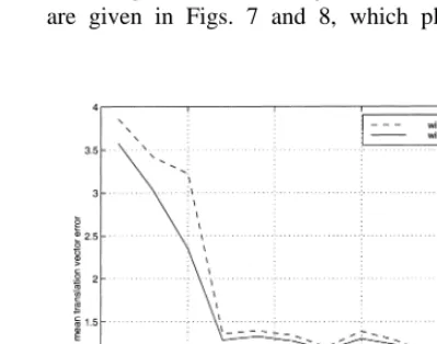
To compare the integrated linear technique with an existing linear technique, we studied its
perfor-Ž .
mance against that of Faugeras 1993 . The results are given in Figs. 7 and 8, which plot the mean
Ž .
Fig. 6. Mean translation vector error mm versus the number of
Ž .
[image:12.595.58.254.423.577.2] [image:12.595.295.495.442.599.2]Fig. 7. Mean rotation vector error versus SNR. The curve for Faugeras’ algorithm was obtained using 10 points, while the curve for the integrated technique was generated using a combination of three points, one line, and one circle.
rotation and translation vector errors as a function of the SNR, respectively.
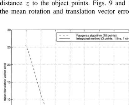
The two figures clearly show the superiority of the new integrated technique over Faugeras’ linear technique, especially for the translation errors. To further compare the sensitivity of the two techniques to viewing parameters, we changed the position pa-rameters of the camera by doubling the camera distance z to the object points. Figs. 9 and 10 plot the mean rotation and translation vector errors as a
[image:13.595.292.498.48.211.2]Ž .
[image:13.595.292.498.392.557.2]Fig. 8. Mean translation vector error mm versus SNR. The curve for Faugeras’ algorithm was obtained using 10 points, while the curve for the integrated technique was generated using a combina-tion of three points, one line, and one circle.
Fig. 9. Mean rotation vector error versus SNR with an increased
Ž
camera position parameter z doubling the camera and object
.
distance z . The curve for Faugeras’ algorithm was obtained using 10 points, while the curve for the integrated technique was generated using a combination of three points, one line, and one circle.
function of SNR respectively under the new camera position. While increasing z causes an increase in the estimation errors for both techniques, its impact on Faugeras’ technique is more serious. This leads to a much more noticeable performance difference be-tween the two linear techniques. The fact that the
Ž .
Fig. 10. Mean translation vector error mm versus SNR with an
Ž
increased camera position parameter z doubling the camera and
.
[image:13.595.53.259.411.578.2]integrated technique using only five geometric enti-Ž
ties three points, one line, and one circle with a total .
of 17 equations still outperforms Faugeras’
tech-Ž .
nique, which uses 10 points a total of 20 equations , shows that the higher-level geometric features such as lines and circles can provide more robust solu-tions than those provided solely by points. This demonstrates the power of combining features on different levels of abstraction. Our study also shows that Faugeras’ linear technique is very sensitive to noise when the number of points used is close to the required minimum. For example, when only six points are used, a small perturbation of the input data can cause significant errors on the estimated parame-ters, especially the translation vector. Figs. 9 and 10 reveal that the technique using only points is numeri-cally unstable to viewing parameters with respect to z.
7.2. Performance characterization with real images
This section presents results obtained using real images of industrial parts. The images contain linear
Ž .
[image:14.595.293.496.48.197.2]features points and lines and non-linear features Žcircles . This phase of the experiments consist of. two parts. First, we visually assess the performance of the linear least-squares framework using different combinations of geometric entities, such as one cir-cle and six points; one circir-cle and two points; and one
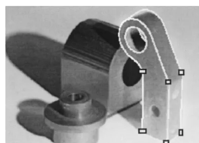
Fig. 11. The alignment between the image of a part and the
Ž .
reprojected outline white of using the exterior orientation
com-Ž .
puted using two points as indicated by the black squares and one
Ž .
[image:14.595.53.259.425.577.2]circle the upper circle with the integrated technique.
Fig. 12. The alignment between the image of a part and the
Ž .
reprojected outline white of using the exterior orientation
com-Ž .
puted using one point, two lines, and one circle the upper circle with the integrated technique. The points and lines used are marked with black squares and lines.
circle, one point and two lines. The performance of the proposed technique is judged by visual inspec-tion of the alignment between the image of a part and the reprojected outline of the part using the estimated transformation matrix. Second, the tech-nique is compared against existing methods that use only one type of geometric entity as well as against
Ž
the Gauss–Newton iterative method similar to the .
bundle adjustment method . Due to unavailability of groundtruth data, the closeness between the solutions from the integrated linear method and from the iterative method, as represented by the residual er-rors, as well as the number of iterations required by the iterative method to converge, are used as mea-sures to indicate the goodness of the solution ob-tained using the new method.
To test the integrated technique, we performed the
Ž .
Fig. 13. The alignment between the image of a part and the
Ž .
reprojected outline white of using the exterior orientation
com-Ž .
puted using six points as indicated by the black squares and one
Ž .
circle the upper circle with the integrated technique.
11–13 that the result using six points and one circle is superior to the ones obtained using the other two configurations.
The significance of these sample results is as follows. First, they demonstrate the feasibility of the proposed framework applied to real image data. Sec-ond, they show that using multiple geometric primi-tives simultaneously to compute the exterior orienta-tion reduces the dependency on points. One can be more selective when choosing which point corre-spondence to use in exterior orientation estimation. This can potentially improve the robustness of the estimation procedure since image points are more susceptible to noise than image lines and ellipses. Third, the use of more than the minimum required number of geometric features provides redundancy to the least-squares estimation, therefore improving the accuracy of the solution, as evidenced by the progressively improved results as the number of linear equations increase.
In order to compare the results with those of other existing techniques, we computed the exterior orien-tation of the same object using the same six points and the same circle, separately. The result for the exterior orientation computation using a linear
tech-Ž . Ž
nique Ji and Costa, 1997 similar to that of Faugeras Ž1993.. with six points is given in Fig. 14. The
Ž .
algorithms of Dhome et al. 1989 and Forsyth et al. Ž1991. for the pose-from-circle computation were
Ž .
augmented in Costa 1997 to handle
non-rotation-Fig. 14. The alignment between the image of a part and the
Ž .
reprojected outline white of using the exterior orientation com-puted using six points alone. It shows good alignment only at the lower part of the object where the concentration of detectable feature points is located and a poor alignment on the upper part of
Ž .
the object as indicated by the arrow .
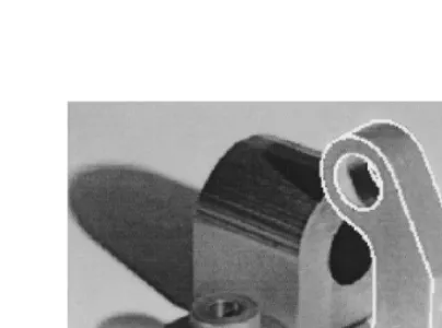
ally symmetric objects. The results of this augmented algorithm using the single ellipsercircle correspon-dence are shown in Fig. 15. Notice that due to the localized concentration of detectable feature points and the physical distance between the circle and these points, the projected outlines computed align well only in the areas where the features used are located. Specifically, the result in Fig. 15 shows a good alignment in the upper portion of the object
Fig. 15. The alignment between the image of a part and the
Ž .
reprojected outline white of using the exterior orientation com-puted using a single circle. It shows a good alignment in the upper portion of the object where the circle is located and a poor
Ž .
[image:15.595.292.497.49.199.2] [image:15.595.292.496.418.567.2]Table 1
Exterior orientations from different methods
Ž .
Method R T mm
0.410 y0.129 y0.902
Ž . w x
Point only Fig. 14 0.606 y0.700 0.376 y43.125 y25.511 1232.036
y0.681 y0.701 y0.208 0.302 0.302 y0.932
Ž . w x
Circle only Fig. 15 0.692 y0.628 0.355 y35.161 y15.358 1195.293
y0.655 y0.753 y0.054 0.398 y0.142 y0.902
Ž . w x
Points and circle Fig. 13 0.554 y0.667 0.336 y43.077 y26.400 1217.855
y0.700 y0.684 y0.201 0.341 y0.156 y0.927
Ž . w x
Bundle adjustment Fig. 16 0.631 y0.693 0.349 y43.23 y28.254 1273.07
y0.697 y0.704 y0.137
where the circle is located and a poor alignment in
Ž .
the lower part as indicated by the arrow . On the other hand, the result in Fig. 14 shows a good alignment only at the lower part of the object where the concentration of detectable feature points is lo-cated and a poor alignment on the upper part of the
Ž .
object as indicated by the arrow .
Visual inspection of the results in Figs. 13–15 shows the benefits of the new technique over the existing methods. The model reprojection using the transformation matrix obtained using the new tech-nique yields a better alignment than those using only points or only ellipsercircle correspondences. To compare the performance quantitatively, we compare the transformation matrices obtained using the three
Ž .
[image:16.595.294.496.437.587.2]methods with different combinations of features against the one obtained from the iterative procedure Žbundle adjustment Table 1 shows the numerical. results for the transformations obtained from using only points, only the circle, and a combination of points and circle. The results from each method were
Table 2
Iterations needed for the bundle adjustment method to converge using the solutions of the three linear methods as initial estimates
Method Number of iterations
Points only 4
Circle only 6
Points and circle 1
then used as the initial guess to the iterative Gauss– Newton method. The final transformation obtained after the convergence of the iterative method is shown in the last row of Table 1. These final results are the same regardless of which initial guess was used. But they vary in number of iterations required as shown in Table 2.
Table 2 summarizes the number of iterations re-quired for the iterative procedure to converge using as initial guesses the results from the three linear methods mentioned in Table 1. Fig. 16 shows the results from the iterative procedure.
[image:16.595.47.263.569.617.2]It is evident from Tables 1 and 2 and Fig. 16 that the new technique yields a transformation matrix that is closer to the one obtained from the bundle adjust-ment procedure and therefore requires fewer
itera-Ž .
tions one here for the bundle adjustment method to converge. By contrast, the final results for initial guesses obtained using only points and only one circle require four and six iterations, respectively, for the bundle adjustment procedure to converge. The result from the quantitative study echoes the conclu-sion from visual inspection: the new technique offers better estimation accuracy, because it is capable of fusing all information available.
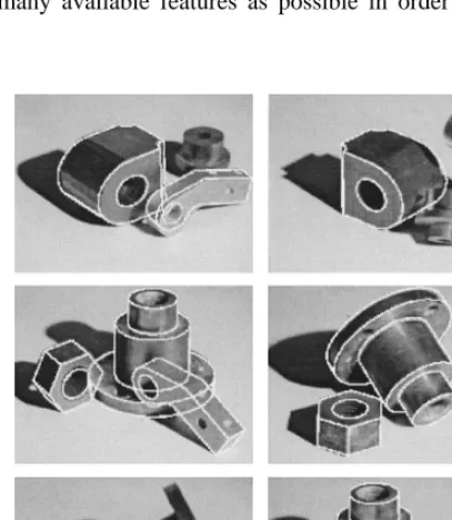
To further validate our technique, we tested it on over 50 real images with similar results. Fig. 17 give results of applying the integrated technique to differ-ent industrial parts with differdiffer-ent combinations of geometric features. Our experiments also reveal, as was theoretically expected for a system of linear equations of the form AXsb, a decay in robustness when the number of equations in the linear system reaches the minimum required for a solution to be found. The premise is that one should make use of as many available features as possible in order to
im-Fig. 17. Results of the integrated method applied to different industrial parts.
prove accuracy and robustness. Our technique fol-lows this principle.
8. Discussion and summary
In this paper, we presented a linear solution to the exterior orientation estimation problem. The main contributions of this research are the linear frame-work for fusing information available from different geometric entities and for introducing a novel tech-nique that approximately imposes the orthonormality constraints on the rotation matrix sought. Experimen-tal evaluation using both synthetic data and real images show the effectiveness of our technique for imposing orthonormal constraints in improving esti-mation errors. The technique is especially effective when the SNR is low or fewer geometric entities are used. The performance study also revealed superior-ity of the integrated technique to a competing linear technique using only points in terms of robustness and accuracy.
[image:17.595.54.258.364.598.2]covariance matrix for each type of feature. The covariance matrices can then used as weightings for different features.
The new technique proposed in this paper is ideal for applications such as industrial automation where robustness, accuracy, computational efficiency, and speed are needed. Its results can also be used as initial estimates in certain applications where more accurate camera parameters are needed. The pro-posed algorithm is more suitable for images with man-made objects, especially in close-range applica-tions.
References
Abdel-Aziz, Y.I., Karara, H.M., 1971. Direct linear transformation from comparator co-ordinates into object–space coordinates. ASP Symp. on Close-Range Photogrammetry, 1–18. Abidi, M.A., 1995. A new efficient and direct solution for pose
estimation using quadrangular targets — algorithm and
evalu-Ž .
ation. IEEE T-PAMI 17 5 , 534–538.
Bopp, H., Krauss, H., 1978. An orientation and calibration method for non-topographic applications. Photogramm. Eng. Remote
Ž .
Sens. 44 9 , 1191–1196.
Chen, S.-Y., Tsai, W.-H., 1990. Systematic approach to analytic determination of camera parameters by line features. Pattern
Ž .
Recognit. 23 8 , 859–897.
Chen, S.Y., Tsai, W.H., 1991. Determination of robot locations by common object shapes. IEEE Trans. Robotics Automation 7
Ž .1 , 149–156.
Costa, M.S., 1997. Object recognition and pose estimation using appearance-based features and relational indexing. PhD Dis-sertation, Intelligent Systems Laboratory, Department of Elec-trical Engineering, University of Washington, Seattle. Dhome, M.D., Lapreste, J.T., Rives, G., Richetin, M., 1989.
Spatial localization of modeled objects of revolution in monocular perspective vision. First European Conference on Computer Vision, 475–485.
Doehler, M., 1975. In: Verwendung von pass-linien anstelle von pass-punkten in der nahbildmessung Festschrift K. Schwidef-sky, Institute for Photogrammetry and Topography, Univ. of Karlsruhe, Germany, pp. 39–45.
Drewniok, C., Rohr, K., 1997. Exterior orientation — an auto-matic approach based on fitting analytic landmark models.
Ž .
ISPRS J. Photogramm. Remote Sens. 52 3 , 132–145. Echigo, T., 1990. Camera calibration technique using three sets of
Ž .
parallel lines. Mach. Vision Appl. 3 3 , 159–167.
Ethrog, U., 1984. Non-metric camera calibration and photo orien-tation using parallel and perpendicular lines of photographed
Ž .
objects. Photogrammetria 39 1 , 13–22.
Faugeras, O.D., 1993. Three Dimensional Computer Vision: a Geometric Viewpoint. MIT Press.
Finsterwalder, R., 1991. Zur verwendung von passlinien bei
pho-Ž .
togrammetrischen aufgaben. Z. Vermessungswesen 116 2 , 60–66.
Fischler, M.A., Bolles, R.C., 1981. Random sample consensus: a paradigm for model fitting with applications to image analysis
Ž .
and automated cartography. Communications ACM 24 6 , 381–395.
Forkert, G., 1996. Image orientation exclusively based on free-form tie curves. Int. Arch. Photogramm. Remote Sens. 31
ŽB3 , 196–201..
Forsyth, D., Mundy, J.L., Zisserman, A., Corlho, C., Heller, A., Rothwell, C., 1991. Invariant descriptors for 3d object recogni-tion and pose. IEEE Trans. PatternAnalysis Machine
Intelli-Ž .
gence 13 10 , 971–991.
Gao, M., 1992. Estimating camera parameters from projection of a rectangular parallelepiped. J. Northwest. Polytechnic Univ. 10
Ž .4 , 427–433.
Haralick, R.M., 1988. Determining camera parameters from the
Ž .
perspective projection of rectangle. Pattern Recognit. 22 3 , 225–230.
Haralick, R.M., Chu, Y.H., 1984. Solving camera parameters from perspective projection of a parameterized curve. Pattern
Ž .
Recognit. 17 6 , 637–645.
Haralick, R.M., Shapiro, L.G., 1993. In: Computer and Robot Vision vol. 2 Addison-Wesley, Reading, MA.
Haralick, R.M., Joo, H., Lee, C., Zhang, X., Vaidya, V., Kim, M., 1989. Pose estimation from corresponding point data. IEEE
Ž .
Trans. Systems, Man Cybernetics 19 6 , 1426–1446. Haralick, R.M., Lee, C., Ottenberg, K., Nolle, M., 1994. Review
and analysis of solutions of the three point perspective pose
Ž .
estimation. Int. J. Comput. Vision 13 3 , 331–356.
Heikkila, J., 1990. Update calibration of a photogrammetric
sta-Ž .
tion. Int. Arch. Photogramm. Remote Sens. 28 5r2 , 1234– 1241.
Heikkila, J., 1991. Use of linear features in digital
photogramme-Ž .
try. Photogramm. J. Finland 12 2 , 40–56.
Holt, R.J., Netravali, A.N., 1991. Camera calibration problem: some new results. Comput. Vision, Graphics Image Processing
Ž .
54 3 , 368–383.
Horn, B.K.P., 1987. Closed-form solution of absolute orientation
Ž .
using quaternions. J. Opt. Soc. Am. A 4 4 , 629–642. Hung, Y., Yeh, P.S., Harwood, D., 1985. Passive ranging to
known planar point sets. Proc. IEEE Int. Conf. Robotics Automation, 80–85.
Ji, Q., Costa, M.S., 1997. New linear techniques for pose estima-tion using point correspondences. Intelligent Systems Lab., Department of Electrical Engineering University of Washing-ton, Technical ReportaISL-04-97.
Kager, H., 1989. A universal photogrammetric adjustment system. Opt. 3D Meas., 447–455.
Kamgar-Parsi, B., Eas, R.D., 1990. Calibration of stereo system with small relative angles. Comput. Vision, Graphics Image
Ž .
Processing 51 1 , 1–19.
Kruck, E., 1984. A program for bundle adjustment for engineering applications — possibilities, facilities and practical results.
Ž .
location and orientation from noisy data having outliers. IEEE Workshop on Interpretation of 3D Scenes, 52–60.
Lee, R., Lu, P.C., Tsai, W.H., 1990. Robot location using single views of rectangular shapes. Photogramm. Eng. Remote Sens.
Ž .
56 2 , 231–238.
Linnainmaa, S., Harwood, D., 1988. Pose determination of a three-dimensional object using triangle pairs. IEEE T-PAMI
Ž .
10 11 , 634–647.
Liu, Y., Huang, T.S., Faugeras, O.D., 1990. Determination of camera locations from 2d to 3d line and point correspondence.
Ž .
IEEE Trans. Pattern Analysis Machine Intelligence 12 1 , 28–37.
Lugnani, J.B., 1980. Using digital entities as control. PhD thesis, Department of Surveying Engineering, The University of New Brunswick, Fredericton.
Ma, D.S., 1993. Conics-based stereo, motion estimation and pose
Ž .
determination. Int. J. Comput. Vision 10 1 , 7–25.
Maas, H.G., 1999. Image sequence based automatic multi-camera system calibration techniques. ISPRS J. Photogramm. Remote
Ž .
Sens. 54 6 , 352–359.
Masry, S.E., 1981. Digital mapping using entities: a new concept.
Ž .
Photogramm. Eng. Remote Sens. 48 11 , 1561–1599. Mikhail, E.M., 1993. Linear features for photogrammetric
restitu-tion and other object complerestitu-tion. In: Proc. SPIE, 1944. pp. 16–30.
Mikhail, E.M., Mulawa, D.C., 1985. Geometric form fitting in industrial metrology using computer-assisted theodolites. ASPrACSM Fall Meeting, 1985.
Mulawa, D., 1989. Estimation and photogrammetric treatment of linear features. PhD dissertation, School of Civil Engineering, Purdue University, West Lafayette, USA.
Mulawa, D.C., Mikhail, E.M., 1988. Photogrammetric treatment of linear features. Int. Arch. Photogramm. Remote Sens. 27
ŽB10 , 383–393..
Okamoto, A., 1981. Orientation and construction of models: Part I. The orientation problem in close-range photogrammetry.
Ž .
Photogramm. Eng. Remote Sens. 47 11 , 1615–1626. Paderes, F.C., Mikhail, E.M., Foerstner, W., 1984. Rectification
of single and multiple frames of satellite scanner imagery using points and edges as control. In: NASA Symp. on Mathematical Pattern Recognition and Image Analysis, Hous-ton.
Petsa, E., Patias, P., 1994a. Formulation and assessement of
straight line based algorithms for digital photogrammetry. Int.
Ž .
Arch. Photogramm. Remote Sens. 5 , 310–317.
Petsa, E., Patias, P., 1994b. Sensor attitude determination using
Ž .
linear features. Int. Arch. Photogramm. Remote Sens. 30 1 , 62–70.
Pettersen, A., 1992. Metrology norway system — an on-line industrial photogrammetric system. Int. Arch. Photogramm.
Ž .
Remote Sens. 29 B5 , 43–49.
Phong, T.Q., Horward, R., Yassine, A., Tao, P., 1995. Object pose from 2-d to 3d point and line correspondences. Int. J.
Ž .
Comput. Vision 15 3 , 225–243.
Rothwell, C.A., Zisserman, A., Marinos, C.I., Forsyth, D., Mundy, J.L., 1992. Relative motion and pose from arbitrary plane
Ž .
curves. Image and Vision Computing 10 4 , 251–262. Shan, J., 1996. An algorithm for object reconstruction without
interior orientation. ISPRS J. Photogramm. Remote Sens. 51
Ž .6 , 299–307.
Strunz, G., 1992. Image orientation and quality assessment in feature based photogrammetry. Robust Comput. Vision, 27–40. Sutherland, I.E., 1974. Three-dimensional data input by tablet.
Ž .
Proc. IEEE 62 4 , 453–461.
Szczepanski, W., 1958. Die loesungsvorschlaege fuer den raeum-lichen rueckwaertseinschnitt. Deutsche Geodaetische Kommis-sion, Reihe C, 29.
Tommaselli, A.M.G., Lugnani, J.B., 1988. An alternative mathe-matical model to the collinearity equation using straight
fea-Ž .
tures. Int. Arch. Photogramm. Remote Sens. 27 B3 , 765–774. Tommaselli, A.M.G., Tozzi, C.L., 1996. A recursive approach to space resection using straight lines. Photogramm. Eng. Remote
Ž .
Sens. 62 1 , 57–66.
Tsai, R., 1987. A versatile camera calibration technique for high-accuracy 3d machine vision metrology using off-the-shelf tv
Ž .
cameras and lens. IEEE J. Robotics Automation 3 4 , 323– 344.
Wang, L.L., Tsai, W.H., 1990. Computing camera parameters using vanishing-line information from a rectangular par-allepiped. Mach. Vision Appl. 3, 129–141.
Wang, X., Xu, G., 1996. Camera parameters estimation and
Ž .
evaluation in active vision system. Pattern Recognit. 29 3 , 439–447.
Weng, J., Huang, T.S., Ahuja, N., 1992. Motion and structure from line correspondences closed-form solution, uniqueness
Ž .