RELATIVE POSE ESTIMATION FROM AIRBORNE IMAGE SEQUENCES
T. Reize a*, R. Müller a, F. Kurz a
The Remote Sensing Technology Institute, German Aerospace Center (DLR), Oberpfaffenhofen, Germany (reize, mueller, kurz)@dlr.de
Commission III, WG III/1
KEY WORDS: Photogrammetry, Image Orientation Estimation Method, Matching, Algorithms, IMU.
ABSTRACT:
We present a new relative pose estimation method for applications based on airborne image sequences. The performance of the method is tested using simulated test data, with correct and erroneous original conditions, as well as using real data. The calculated results obtained from real images are compared to the on-board measured angles. The results show that the proposed method is very precise and fast. Most matching algorithms are very computation time expensive mainly because they rely on RANSAC methods that need a lot of matching points. Due to the circumstance that only two corresponding points are necessary to solve the equation system, our technique doesn’t need much computation time. Outliers are detected by a special back-matching technique. A method based on Polynomial Homotopy Continuation (PHC) is used to solve the complex polynomial equation system. The proposed pose solver method runs without SVD calculations, expensive minimisation or optimisation. Start parameters are not necessary. Furthermore, no a priori knowledge is required, besides focal length in pixel units and overlapping consecutive images. Outcomes are three relative orientation angles and a scaling parameter between two subsequent images, as well as displacement vectors in image pixel coordinate units. In addition, the PHC pose estimation method can balance small pixel errors. All these properties indicate the high applicability of the proposed method.
1. INTRODUCTION
Relative poses describe the orientation and position of an image relative to another image. Poses can be measured at the time of image exposure or estimated by calculations from overlapping image sequences.
1.1 Motivation
Relative poses can be a preliminary stage towards absolute pose estimation, image registration, 3D reconstruction and orthorectification. Müller (Müller, 2005) demonstrated an image registration and rectification process of airborne images using onboard pose measurements.
Precise airplane navigation angle measurements are usually achieved by an Inertial Measurement Unit (IMU), a costly and heavy device. We aim to replace this device by using only the available image information and calculate the pose angles in near real time. An important intermediate step towards this challenging task is the development of a fast and accurate relative pose estimation method.
1.2 Previous Work
Different pose estimation methods are known in photogrammetry and computer vision. Most solutions are based on finding corresponding matching points between images and solving an equation system with coplanar conditions.
--- *
Corresponding author: [email protected]
Several approaches with different amount of matching points are known in the literature, but all suffer from the problem of finding roots to a polynomial equation system (Ameller, 2002), (Brückner, 2008), (Horn, 1990), (Horn, 1991), (Kukelova, 2008), (Nister, 2004), (Nister, 2006), (Quan, 1999), (Rodehorst, 2008). Other solutions focus on iterative methods by stepwise minimizing a cost function which can be very runtime consuming and global minima are difficult to find (Lee, 2004), (Lu, 2000). All solutions can be optimized by bundle adjustment procedures, but with loss of application possibilities for real-time requirements (Agarwal, 2010), (Crandall, 2011).
1.3 Our Work
We propose a different method to determine relative poses from images. The entire algorithm relies on Polynomial Homotopy Continuation (PHC) methods (Verschelde, 1999), (Verschelde, 2010), (Zulehner, 1988). The PHC method is employed to solve the polynomial equation system arising from the usual Helmert Transformation.
2. METHOD
The relative pose estimation method operates on a subsequent, overlapping airborne image pair. Once the calculation loop, described below, has finished, the second image will be used as first image for the next subsequent, overlapping image pair.
2.1 Estimating translation
In a first step the translation in the image frame is estimated. Since the image’s projection center is not known, we use the
image center in the first image to create a Normalized Cross Correlation (NCC) model and find it in the second image. The model’s centers serve as corresponding points and by taking the difference in row and column the translation in the image frame can be roughly estimated. This assumption is valid for a camera’s principal point located in the airplane’s center of gravity. In this case the image’s center equals the center of rotation. The displacement vector n+1
n
T is defined as a 2 by 1
vector in the camera frame and given in pixel units.
2.2 Image matching
In the first image a point described by row and column is determined, at random. The area of around 50 to 150 pixels that encircles that point creates the NCC model, which is subject to be located in the second image provided the correlation coefficient is above a chosen threshold value. The model’s centers serve as matching points again. Subsequently a back-matching process is invoked, where in the second image at the location of the found matching point a new NCC model of different size is created and located in the first image. If this model’s center found by back-matching and the randomly chosen point in the first image is less than one pixel separated in distance, the point will be accepted as a pair of corresponding points. The corresponding points of the first image’s center and its location in the second image, as described in section 1.2, are used again as matching points. The back-matching procedure increases the computation time, but highly supports outlier detection and removal. In a last step, the corresponding points are mapped to the three dimensional vectors n
q1, n
q using the focal length f in pixel units as z-component.
2.3 The system of equations
The following approximation is used in order to describe the image transformation pixel by pixel:
1
Q is presented by the unit quaternion description (a, b, c, d).
The displacement vector n+1
n
T is defined in two dimensions whereas the equation system (1) requires three dimensions. This problem is dealt with by using only the first and the second equation of the entire system. Equation (1) contains five unknownsv= (a, b, c, d, s).
The scaling parameter 1( )
h sn
n ∆
+ depends on the difference in
flight altitude Δh. n+1
n
Q describes the rotation between image n
and image n+1 in the quaternion representation and consists of the four quaternion parameters (a, b, c, d).
Equation (1) refers to an approximated version of the usual Helmert Transformation, since the scaling parameter 1( )
h sn
n ∆
+
relates to the pixel located at the unknown projection center and will be slightly different for other image positions, if the airplane’s navigation angles were non-zero at the time of image exposure. Further, the scaling parameter 1( )
h sn
n ∆
+ depends on
difference in flight altitude over ground Δh and regions of steep or rugged terrain will cause changing scaling parameters in a single image. The last is a condition difficult to fulfill. Nevertheless, with the assumption of small navigation angles and flat terrain, equation (1) serves as a good approximation. As explained above the z-component equation is discarded and the resulting equations form the following equation systemH(v)
with the parameter vector of unknowns v=(a,b,c,d,s).
2.4 Root finding with PHC
Root finding in higher dimensional polynomial systems is a difficult problem. We tested the freely available software package PHCpack and found that PHC is a very suitable tool to solve our polynomial problem, not only because of its low computational costs, but also because of the reliable extraction of all isolated, complex solution approximations to an n-dimensional polynomial systemH(v). The vectorvcontains all unknown variables as components. The method extends the original polynomial systemH(v)to the equation systemG(v,t), witht∈
[ ]
0,1. In turn, G(v,t) is separated into the targetequation systemH(v)and a simple equation system Pn(v) with the same topological structure.
0
The start equation system
0 ) (v =
Pn (5)
has a well-known set of solutions for n=0. γ is a complex number that guarantees regularity of the solution paths.
If t=0 the equation system G(v,t)equals the start system This new solutions yield the next version of the equation systemG(v,t), including the slightly more complex
In our case 16 solutions remain, whereupon one solution gives the approximated relative image orientation angles.
2.5 Selecting the best solution
Solution extraction is a crucial part in our pose estimation. The selection procedure includes two main criteria:
First, some solutions are discarded due to the condition that the scaling parameter should be close to one. For example if there’s no change in flight altitude above ground from image to image,
the scaling parameter should equal one. Height differences are very small in comparison to the flight height over ground in our application. Therefore the scaling parameter can be restricted to an interval of [0.8, 1.2].
Second, a complex solution actually is not a physical solution. Hence we select the solution with the smallest imaginary part out of the remaining results. Usually there are solutions with imaginary parts as small as ≈10e-130 or less.
Another selection feature is provided by real part of the quaternion angle parameter a, that must be smaller than one and should be close to one for small rotations.
2.6 Conversion to navigation angles
In a final step the determined quaternion is converted into the Euler rotation angle representation that describes the relative orientation between two images.
Now, step 1- 6 continues with the next image pairs for a given sequence of images.
3. RESULTS 3.1 Results with simulated data
In order to test the PHC method a system of equations with perfect corresponding points, calculated with equation (1) has been used. For this purpose, two random points n
q1and n
q2 have been chosen and transformed by a known rotation, scaling and transformation into the corresponding points 1
1
+ n
q and 1
2
+ n
q .
These exact corresponding points, together with the known translation were used in equation (3). The PHC pose estimation method found the correct angles and scaling.
The test proceeded with perfect Roll, Pitch and Yaw angles varying from -45° to +45°. In doing so, the solution selection criteria have been monitored simultaneously. Figure 1 shows the resulting deviation of correct original angles and calculated angles in degrees. In this test with exact calculated corresponding points, results gained by the PHC pose estimation method showed to be very precise and reliable.
Figure 1. Difference between PHC-calculated relative angles and original, simulated angles varying from -45° to 45°.
The PHC method for polynomial root finding has been proved to be a very suitable approach for relative pose estimation at least with perfect original conditions.
3.2 Results with noisy simulated data
The simulation with exact conditions, described in section 3.1, has been used again to verify the pose estimation method in the
presence of improper original conditions. The method has been tested while the exact corresponding points were subject to artificial uncertainties. An offset, varying from 1 to 50 pixels, has been added and the results were compared to the relative angles obtained without error offset. Results with shifts up to 50 pixels and a typical relative angle configuration of Roll=-2°, Pitch=-1.5° and Yaw=3.2° are illustrated in figure 2. The IMU performance specification of 0.01° in Roll/Pitch and 0.1° in Yaw is marked.
Further tests have shown that an error offset for the matching point’s x components, purely add up to the Pitch deviation shown in figure 2. And, vice versa, error offsets in the y components of the matching points result in the illustrated Yaw deviation. An error of 1 Pixel in x direction causes a Pitch angle error of around 0.008°. The same relation holds for Pixel errors in y direction and the Yaw angle.
Figure 2. Shift from 1 to 50 pixels have been added to simulated matching points and relative angles were calculated for a typical configuration of Roll=-2°, Pitch=-1.5°, Yaw=3.2°.
The deviations of calculated and original angles are shown.
Analogous to tests with incorrect corresponding points further test series with erroneous translations and erroneous scaling have been accomplished and compared again to the results obtained from error-free and perfect conditions. Translation vector errors of the x component were visible as Pitch offsets again and y component errors as Yaw offsets. Translation error findings equal the matching point error results shown in figure 2.
3.3 Results with real data
The performance of the relative pose estimation method has been tested with real airborne image scenes, acquired by the DLR 3K system consisting of 16 Mega-Pixel commercial Canon EOS cameras (Kurz, 2007), (Rosenbaum, 2010). The images chosen for this article were gathered over Central Munich with a flight altitude of about 1500 m above ground and a scene overlapping area of around 75% for subsequent images. The ground sampling distance (GSD) is about 20 cm/pixel. Images were taken with a frequency of 2 Hz. An IMU, initialized in a right handed system, is part of the 3K system payload. The angles are defined as follows: Roll around the flight direction x, Yaw around the optical axis z and angle Pitch around axis y completes the right handed system. Producer’s IMU performance specifications of 0.01° in Roll / Pitch and 0.1° in Yaw allow a good comparison of measured and calculated relative poses. Figure 3 shows the used images from two flight tracks over Munich City.
Figure 3. Mosaics produced with two airborne 3K-image scenes gathered over Munich city, overlaid over Google earth®.
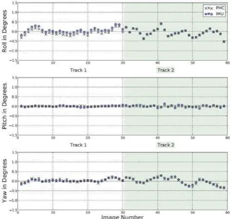
In Figure 4 measured and calculated relative pose angles are compared. Calculations were performed with a NCC model using a radius of 70 pixels and a correlation threshold of 0.9.
Figure 4. Calculated and measured relative pose angles for track 1 (white) and track 2 (green).
Mean value deviations and standard deviations are shown in table 1.
Table 1. Accuracy of the relative pose estimation method tested on real data.
Mean value deviation
Standard deviation
Maximum deviation Roll Track 1 0.124° 0.009° 0.142°
Track 2 0.011° 0.011° 0.027° Pitch Track 1 -0.004° 0.031° -0.081°
Track 2 -0.007° 0.061° 0.123° Yaw Track 1 0.026° 0.031° 0.085° Track 2 0.006° 0.051° -0.123°
The entire algorithm took 2.66 seconds per image pair in average on a quad core system, whereat no parallel processing is implemented in the codes, yet. The CPU works with 2.83GHz and 8106808 kB RAM.
3.4 Discussion
Tests with error-free original conditions showed that the navigation angles calculated by the PHC method are very accurate. Roll Pitch and Yaw deviations are in the range of -0.0001° to -0.0001°. These small internal errors can be neglected for our purpose.
Results obtained from perfect origin conditions have been compared to results subject to inaccurate corresponding points, as well as to inaccurate translations and scaling. Test were performed with a typical navigation angle configuration of Roll=-2°, Pitch=-1.5° and Yaw=3.2°. The deviation behaviours show similar results, both on tests with erroneous corresponding points and on tests with incorrect translations. The angle deviations increase almost linearly with the added shift extensions. In the presence of translation and matching errors the Pitch remains nearly unchanged in accuracy. Further it can be concluded that, depending on relative angle configurations, inaccuracies act different on the three orientation angles. The PHC pose solver outperforms the IMU performance specification of 0.01° in Roll angles, if the error offset of corresponding points is less than 4 pixels. The calculated Yaw exceeds the IMU Yaw specified performance tolerance of 0.1°, if the corresponding point error is less than 11 pixels. The calculated Pitch angles remain more precise for more then 52 pixels offset then the IMU performance specification of 0.01°.
The algorithm has been tested with real airborne images. Tests with real data sometimes give rise to a constant Roll offset. In track 1 a nearly constant offset of ~0.1° on average appears with a standard deviation of only 0.009°. Up to now, we do not know the source of this scene-dependent offset. In contrast all other average angle deviations are below 0.02° and standard deviations remain between 0.01° and 0.06°, giving rise to a statistical error source. Besides this effect the method is robust against outliers and average deviations of ~0.01° are acceptable. Real data tests with images taken from other flight campaigns achieve similar accuracies.
With 2.66 seconds per image pair, the algorithm is already very fast, even if not prepared for speed, yet.
4. CONCLUSION
We have presented a closed-form relative pose estimation method. A specific feature is allegorised by the root finding method PHC.
Outlier detection is already included in the matching process with the back-matching technique. Though this costs additional computational time, it secures the stability and reliability of the entire algorithm. Thus, no costly statistical optimization methods, like e. g. RANSAC, need to be applied to the results.
Tests with error-free matching points and an exact scaling and translation proved the reliability of our method and errors of less than 0.0001° can be neglected. Continuative tests showed the behaviour of PHC calculated angles in the presence of erroneous corresponding points and translations.
Applied on real image data sets the PHC pose solver method proved of value. Average deviations are less than 0.1°. The PHC calculated Yaw angle outperforms the IMU measured Yaw angle in accuracy.
The entire algorithm, including matching, takes around 2.66 seconds per image pair, each image with 16 Mega-Pixels. We believe that our method can be optimized in accuracy and speed. Especially, whenever pose estimation applications require real-time conditions the PHC pose estimation method might be of interest.
4. ACKNOWLEDGEMENT
We gratefully appreciated personal communication and discussions with Peter Reinartz, Oliver Meynberg, Dominik Rosenbaum, Jens Leitloff and Georg Kuschk.
5. REFERENCES References from Journals:
Agarwal, S., Furukawa, Y., Snavely, N., Curless, B., Seitz, S., M., Szeliski, R., June 2010. Reconstructing Rome. IEEE
Xplore.
Bückner, M., Bajramovic, F., Denzler, J., 2008. Experimental Evaluation of Relative Pose Estimation Algorithms. Proc.
Computer Vision Theory and Application – VISAPP (2), pp.
431-438.
Horn, B., K., P., 1990. Relative Orientation. International
Journal of Computer Vision, Vol. 4, pp. 59-78.
Horn, B., K., P., 1991. Relative Orientation Revisited. Journal
of the Optical Society of America A, Vol. 8, pp. 1630-1638.
Lu, C., P., Hager, G., D., June 2000. Fast and Globally Convergent Pose Estimation from Video Images. IEEE Trans.
Pattern Analysis and Machine Intelligence, Vol. 22, No. 6.
Nister, D., June 2004. An efficient Solution to the Five-Point Relative Pose Problem. IEEE Trans. Pattern Analysis and
Machine Intelligence, Vol. 26, No. 6.
Quan, L., Lan, Z., Aug. 1999. Linear N-Point Camera Pose Determination. IEEE Trans. Pattern Analysis and Machine
Intelligence, Vol. 21, No. 8.
Stewenius, H., Engles, C., Nister, D., June 2006. Recent Development on Direct Relative Orientation. ISPRS Journal of
Photogrammetry and Remote Sensing, Vol. 60, Issue 4, pp.
284-294.
Verschelde, J., 1999. Algorithm 795: PHCpack: A general-purpose solver for polynomial systems by homotopy continuation. ACM Trans. Math. Softw. 25(2), pp. 251-276.
Zulehner, W., Jan. 1988. A Simple Homotopy Method for Determining All Isolated Solutions to Polynomial Systems.
Mathematics of Continuation, Vol. 50, No. 181, pp. 167-177.
References from Other Literature:
Ameller, M., A., Triggs, B., Quan, L., 2002. Camera Pose Revisited – New Linear Algorithms, 13’eme congress Francophone AFRIF-AFIA de Reconnaissance de Formes et
Intelligende Artificielle.
Crandall, D., Owens, A., Snavely, N., Huttenlocher, D., 2011. Discrete-continuous optimization for large-scale structure from motion, IEEE CVPR Conference 2011, Colorado Springs, USA.
Kukelova, Z., Bujnak, M., Pajdla, T., 2008. Polynomial Eigenvalue Solutions to the 5-pt and 6-pt Relative Pose Problem, BMVC.
Kurz, F., Müller, R., Stephani, M., Reinartz, P., Schroeder, M., 2007. Calibration of a wide-angle digital camera system for near real time scenarios, ISPRS Hannover Workshop 2007, High
Resolution Earth Imaging for Geospatial Information, ISSN
1682-1777.
Lee, P., Y., Moore, J., B., 2004. Pose Estimation via Gauss-Newton-on-manifold Approach. Proc. Of the 16th International
Symposium on Mathematical Theory of Networks and Systems,
Leuven, Belgium.
Müller, R., Lehner, M., Reinartz, P., Schroeder, M., 17.-20. Mai 2005. Evaluation of Spaceborne and Airborne Line Scanner Images using a Generic Ortho Image Processor, High
Resolution Earth Imaging for Geospatial Information,
Hannover, Germany, Vol. XXXVI, ISBN ISSN No. 1682-1777.
Rodehorst, V., Heinrichs, M., Hellwich, O., 2008. Evaluation of Relative Pose Estimation Methods for Multi-Camera Setups.
International Archives of the Photogrammetry, Remote Sensing
and Spatial Information Sciences, Beijing, China, Vol. 37-B3b,
pp. 135-140.
Rosenbaum, D., Leitloff, J., Kurz, F., Meynberg, O., Reize, T., July 2010. Real-Time Image Processing for Road Traffic Data Extraction from Aerial Images. Proceedings of ISPRS Technical
Commission VII Symposium XXXVIII(7B), ISSN 1682-1777,
pp. 469-475.
Verschelde, J., Yoffe, G., 2010. Polynomial Homotopies on Multicore Workstations, PASCO 2010, Proceedings of the 2010 International Workshop on Parallel Symbolic Computation,
Sierre, Switzerland, pp. 131-140, ACM 2010.
References from websites:
PHCpack: http://www.math.uic.edu/~jan