IMPROVING 3D LIDAR POINT CLOUD REGISTRATION USING OPTIMAL
NEIGHBORHOOD KNOWLEDGE
Adrien Gressin, Cl´ement Mallet, Nicolas David
IGN, MATIS, 73 avenue de Paris, 94160 Saint-Mand´e, FRANCE; Universit´e Paris-Est (firstname.lastname)@ign.fr
Commission III - WG III/2
KEY WORDS:point cloud, registration, ICP, improvement, eigenvalues, dimensionality, neighborhood
ABSTRACT:
Automatic 3D point cloud registration is a main issue in computer vision and photogrammetry. The most commonly adopted solution is the well-known ICP (Iterative Closest Point) algorithm. This standard approach performs a fine registration of two overlapping point clouds by iteratively estimating the transformation parameters, and assuming that good a priori alignment is provided. A large body of literature has proposed many variations of this algorithm in order to improve each step of the process. The aim of this paper is to demonstrate how the knowledge of the optimal neighborhood of each 3D point can improve the speed and the accuracy of each of these steps. We will first present the geometrical features that are the basis of this work. These low-level attributes describe the shape of the neighborhood of each 3D point, computed by combining the eigenvalues of the local structure tensor. Furthermore, they allow to retrieve the optimal size for analyzing the neighborhood as well as the privileged local dimension (linear, planar, or volumetric). Besides, several variations of each step of the ICP process are proposed and analyzed by introducing these features. These variations are then compared on real datasets, as well with the original algorithm in order to retrieve the most efficient algorithm for the whole process. Finally, the method is successfully applied to various 3D lidar point clouds both from airborne, terrestrial and mobile mapping systems.
1 INTRODUCTION
Lidar systems provide 3D point clouds with increasing accuracy and reliability. When the same area of interest is acquired twice, or more, over time or space, depending of the application, the registration problem arises. For airborne or mobile platforms, the use of an hybrid INS/GPS georeferencing system results in 3D shifts between strips or surveys, that come from drifts of the iner-tial measurement unit or GPS signal gaps. For terrestrial devices, registration is required when several points of view of the same object are acquired, facing the issue of putting them in correspon-dence with few overlapping areas.
The Iterative Closest Point (ICP) algorithm is one of the most widespread method to compute registration of two point clouds, with the assumption of the existence of a good a priori alignment. The simplicity of this method, introduced by (Chen and Medioni, 1992) and (Besl and McKay, 1992), is the reason for its extensive use for a large variety of datasets and contexts. Nevertheless, due to sensibility of the iterative method to noise and poor iteration, many variants have been developed to improve all steps of the ICP (Rusinkiewicz and Levoy, 2001). According to (Rodrigues et al., 2002), no optimal solution exists, and the ICP method re-mains a state-of-the-art algorithm (Salvi et al., 2007). In paral-lel, many interesting local descriptors, based on the geometrical point cloud analysis have been elaborated, and successfully used on ICP variants. For instance, (Bae and Lichti, 2008) have re-cently focused on the analysis of the geometrical curvature and the position uncertainty of laser scanner measurement. The intro-duction of features of interest seems indeed very effective, since it allows to focus the registration process on the most reliable re-gions. The ”reliability” may be evaluated according to planar cri-teria or with scale-space analysis (Sharp et al., 2002). For more complex environments with specifics patterns, other primitives may be introduced: the method of (Rabbani et al., 2007), de-signed for industrial areas, relies on various shapes such as planar patches, spheres, cylinders and tori. More generally, Demantk´e
et al. (2011), similarly to Brodu and Lague (2012), have devel-oped a multi-scale analysis of lidar points, based solely on the 3D information. Such analysis allowed them to retrieve for each point the optimal neighborhood size and the prominent behaviour of the vicinity (linear, planar, or volumetric). Our goal is there-fore to introduce such geometric primitive knowledge in the ICP registration procedure using this local geometrical analysis. For the case of roughly aligned datasets, the ICP method provides a rather robust, fast, and accurate result for fine alignment step. Since we focus on pair-wise registration of datasets that do not exhibit large changes (especially in rotation), the coarse 3D reg-istration issue is beyond the scope of this article.
In this paper, the geometrical features of interest are first pre-sented (Section 2). Then, the four steps of the ICP algorithm are described in Section 3. For each step, the introduction of the proposed features is discussed. After a short presentation of the datasets in Section 4, the different variants of the ICP algo-rithm are evaluated and compared in Section 5. Finally, an opti-mized combination of ICP variants is proposed, and conclusions are drawn in Section 6.
2 GEOMETRICAL FEATURES
2.1 Dimensionality features
For a given radiusr, and its associated spherical neighborhood Vr
, a Principal Component Analysis is performed to obtain three eigenvalues(λ1, λ2, λ3), such asλ1 ≥λ2 ≥λ3 ≥0, and three eigenvectors(−→v1,−→v2,−→v3). One can notice that−→v3 provides a ro-bust value of the normal of the 3D point, noted−→n. The standard deviation along an eigenvectoriis denoted by:
∀i∈[1,3], σi=
√
λi. (1)
The shape ofVr
is then represented by an oriented ellipsoid. Three geometrical features are introduced in order to describe the linear (a1D), planar (a2D) or scatter (a3D) behaviors withinVr:
This allows to consider them as the probabilities of each point to be labeled as linear (1D), planar (2D) or volumetric (3D). These low-level primitives are considered to be sufficient to coarsely describe the main behaviours within a point cloud. Since the method is designed to be independent to any information about the acquisition process (objects, point density, scan pattern etc.), additional geometrical description would introduce noise in the process and make the process less general. For the specific case of airborne laser scanning, the reader should refer to (Jutzi and Gross, 2009) where a more complete analysis is performed on which kinds of geometrical behaviours can be detected and la-beled. The dimensionality labeling (1D, 2D, or 3D) ofVr
is
de-results to 1. This corre-sponds to edges between planar surfaces, poles, traffic lights, tree trunks etc. Conversely, in case of planar surface or slightly curved areas,σ1, σ2≫σ3, anda2Dwill prevail. Finally,σ1≃σ2≃σ3
impliesd∗(Vr) = 3
(vegetation, spatially scattered objects etc.).
2.2 Optimal neighborhood radius
The dimensionality features are computed for increasing radii values between a lower boundrminto an upper boundrmax,
us-ing a square factor. Demantk´e et al. (2011) describe how these bounds can be automatically retrieved and how the[rmin, rmax]
space can be efficiently discretized.
For each radiusr, and for each point P, a measure of unpre-dictability is given by the Shannon entropy of the discrete proba-bility distribution(a1D, a2D, a3D):
Ef(Vp) =r −a1Dln(a1D)−a2Dln(a2D)−a3Dln(a3D). (4)
Then, the optimal neighborhood radius is obtained as the mini-mum the entropy functionEf (cf. Figure 1):
r∗P = arg min r∈[rmin, rmax]
Ef(VPr). (5)
The optimal neighborhoodV∗
, associated tor∗is finally used to compute a dimensionality labelingd∗
(Vr∗
Various features have been computed in the previous sections, and several other can be derived from these ones. One main fea-ture of interest is the omnivarianceV (Gross and Thoennessen,
2006), which is the product of theσi, thus proportional to the
ellipsoid volume. It allows to characterize the shape of the neigh-borhood, and, in particular, to enhance whether one or two eigen-values are prominent.
V = Y
i∈[1,3]
σi. (6)
Finally, each 3D point of the cloud can be described by the fol-lowing features:
In practice, only the features considered as the most discrimina-tive have been retained for ICP. They are:
(−→n , d∗, r∗, E∗f, V). (8)
One can note that−→n andV have been computed from the optimal neighborhood, and thus also benefit from the described method. −
→nprovides a robust approximation of the point normal.V allows a global description of the shape of the neighborhood. Since the λiare correlated, they are not conserved.
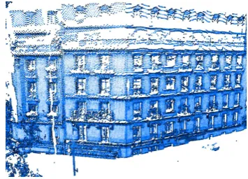
Figure 1 gives an illustration of the entropy feature for a building facade acquired with a Mobile Mapping System.
Figure 1: EntropyE∗
f : 0 (light blue)→1 (dark blue).
3 OPTIMIZING ICP 3.1 ICP steps
The purpose of Iterative Closest Point algorithm is to perform the registration of two coarsely aligned point clouds (amobile point cloud registered on areferencepoint cloud). The algorithm is composed of four steps. First, a reduced number of points is selected to find suitable candidates for registration. Then, match-ing points are found between the two points clouds, and each corresponding pair is weighted. Furthermore, an error metric is traditionally designed with respect to the context and the area of interest, and finally minimized, providing transformation param-eters (translation and rotation). For each step, various existing variants exist (Rusinkiewicz and Levoy, 2001).
Selectionaims to sample the initial point cloud in order to reduce computation time caused by large data sets. Efforts on efficient selection will be performed here.
(Godin et al., 1994) or normals (Pulli, 1999). Since, no underly-ing surface can be considered in our datasets, we have adopted the point-to-point strategy, and did not modify it.
Weighting / Rejectingconsists in adding some contextual knowl-edge for each corresponding pair of interest. Firstly, each of them can be weighted with respect to the neighborhood or the global point cloud. Our features of interest are likely to be relevant for this step. Secondly, the worst pairs may be rejected using, most of the times, statistics on the whole point cloud. Improvements will also be proposed here.
Minimizing.Given a set of matching pointsC={(Pimob, Piref)}i
of two point clouds (mobile&reference) weighted withwi, the
purpose to the last step of the ICP algorithm is to find the transfor-mationT minimizing the sum of the squared distances between each couple of points. The two most frequently adapted distances in the literature are the point distance, and the point-to-plane distance using the normal of each point. Since the local normal vector is assumed to be reliable thanks to the adopted multi-scale analysis, the second option is adopted. The optimal transformationT∗
No further improvement is proposed.
3.2 Selection step
A naive strategy is to randomly subsample the point cloud so that the general distribution of the points is preserved (Turk and Levoy, 1994). As a multi-scale analysis, different samples can also be performed at each iteration (Masuda et al., 1996). Another strategy is to select points with high intensity gradient if color or intensity is available (Godin et al., 1994). Rusinkiewicz and Levoy (2001) prefer selecting points so as to preserve a dis-tribution of normals as large as possible.
As alternatives, two solutions based on our geometrical features of interest are proposed. Two features allow to focus the selection step on the most reliable areas for accurate registration. An area is considered as ”unreliable” if it corresponds to (1) the bound-ary between several objects or surfaces, or to (2) a geometrically complex object. In such cases, since the acquisition processes of the two point clouds may be distinct, the local geometries are likely to be dissimilar. Lines are traditional strong cues for regis-tration, but with the adopted method, they will be discarded.
• High-entropy selection: As described in Section 2.2, the larger Ef∗, the more prominent a single dimension. This
means that the local geometry is simple enough to take a strong decision, thus designing salient regions of the 3D point cloud (Figure 1).
• Dimensionality-based selection: Linear behaviours corre-spond to border between surfaces and thin objects (Demantk´e et al., 2011). It is preferred to remove them from the follow-ing steps of the ICP algorithm. The same conclusion can be drawn with scattered objects, such as vegetation that will not have the same sampling, depending on the point of view.
3.3 Weighting step
After searching corresponding pairs, each of them is weighted. Several weighting functions of two points(P1, P2)exist in the lit-erature (Godin et al., 1994). The basic one is the constant weight-ing functionwC(P1, P2) =w0,w0being arbitrarily set.
Another strategy consists in adding a weighting functiond:
wD(P1, P2) = 1−d(P1,P2)
dmax , wheredmaxis the maximum value
of this function for the set of pairs.
The Euclidian normd(.) = d2(.) = k.kis often used. Since specific geometrical features have been introduced, an omnivari-ance compatibility metricdV(p1, p2)is first proposed. It is based
on the difference of the ellipsoid volumesV. Thus, a weighting functionwV(P1, P2)is designed as follows:
wV(P1, P2) = 1−
Furthermore, normal compatibility can be inserted to define an-other weighting function: wN(P1, P2) =−n1.→−→n2. Since normal
computation has been improved using the method of (Demantk´e et al., 2011), this solution is also tested.
3.4 Rejecting step
The literature generally proposes to reject the worst correspond-ing pairs, based on various distance criteria:
• distance threshold;
• distance more than2.5times the standard deviation of dis-tances of pairs (Masuda et al., 1996);
• rank filter: n% with the greatest distance (Pulli, 1999).
The rejection distance is not necessary the same as for the match-ing step. Here,dV is adopted in order to discard the worst
corre-sponding pairs:
• n% with the greatest distance, usingdV.
4 DATASETS
Three kinds of lidar datasets are exploited in order to assess the relevance and performance of each proposed variant of the algo-rithm. These datasets have various point densities, point distri-bution, and points of view since they have been acquired with different lidar systems: airborne (ALS), terrestrial static (TLS), and mobile mapping systems (MMS).
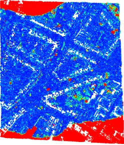
ALS This dataset has been acquired over a dense urban area (city center with low-elevated buildings, cf. Figure 2). Two strips from two different dates are used. Furthermore, each strip was ac-quired with distinct airborne lidar scanners, resulting in two dif-ferent ground patterns. The proposed method will be tested on an overlapping area. The first acquisition (ALS 03) was completed in 2003 (point density of 5 pts/m2,400,000pts, very irregular spatial sampling) with a Toposys fiber scanner. The second ac-quisition (ALS 08) occurred in 2008 (point density of 2 pts/m2,
90,000pts, oscillating mirror) with an Optech 3100 EA device. In such a case, the registration allows to compute high accuracy change map, and is a key step for 3D change detection methods.
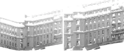
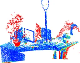
TLS The second dataset (TLS) concerns an indoor environment (point density of 0.3 pts/cm2,20,000pts). Two points of view of the same area (office desk covered with various objects) were consecutively acquired with the same Trimble system (Figure 3).
Figure 2: ALS dataset. Left: ALS 03. Right: ALS 08, colored with respect to the altitude (low (blue)→high (red)).
Figure 3: TLS dataset, with two points of view, colored using ambient occlusion.
masks). Thus, a registration is required. The point cloud den-sity is very variable, even inside the same point cloud, depending on the angle of incidence of the variable distance between ob-jects and the MMS. However, the typical density on the facades of the buildings is near 100 pts/m2(around200,000pts per point cloud). This fluctuating density is another challenge for the reg-istration step.
Figure 4: MMS dataset colored using ambient occlusion: two acquisitions of the same area, but with a temporal shift.
5 EXPERIMENTS
Firstly, the comparison protocol will be detailed. Then, it will be applied at each proposed variant of the ICP algorithm, in order to evaluate each of them, and find the best proposition. Therefore, fifteen different solutions have been tested on three datasets. All of them are presented and commented, but variants with the worst results are not illustrated.
5.1 Comparison method
Point cloud registrations can be compared by straightforwardly computing, for eachmobilepoint cloud, the mean of the distances of the closest points in thereferencepoint cloud. Nevertheless, non-overlapping areas may exist: this value is thus not relevant for that purpose.
To address this issue, then-resolutionRnof a point cloud is
de-fined by the mean distance of then-closest points in the same cloud. In our experiments, the valuen = 5is selected, even if
the selection of the optimal neighbors would have been a better solution. Then, a distance thresholdt= 10× Rnhas been
intro-duced, and the mean of the distances smaller thant(noted¯t) is computed. Finally, the performance of each variant is evaluated through a graph of the variations oft¯with respect to the number of iterations (i.e., the convergence speed), computed on a Intel Core2 2.83GHz CPU with 4GB of RAM. These results are com-pared with adefaultconfiguration, considered at each stage of the registration process. Such a configuration is:
• Selection: all 3D points; • Matching: closest point; • Weighting: constant weightwC;
• Rejecting: none, all corresponding pairs;
• Minimizing: point-to-point distance, without normal com-putation.
5.2 Selecting
Four variations discussed in Section 3.2 have been selected, and are analyzed here. The point cloud is first randomly sampled (random): 10% of the points are conserved. Then, only the 3D points with high entropy values (E∗
f) are selected. Two
thresh-olds are tested: Ef∗ >0.6, andE
∗
f >0.7. Finally, points with
locally linear and scattered behaviours are discarded, resulting in an additional variant: points withd∗= 2. Results are presented in Figure 5.
Figure 5: Results of the Selection step.
The first conclusion is that faster and more accurate registrations can be achieved with proposed selection variants. In this step, the most effective attribute is, for the three datasets, the dimension-ality featured∗, which allows to focus on planar surfaces. Both improvements are noticed for the ALS and TLS datasets. For the MMS dataset, there are only slight differences with thedefault configuration, which is still a valid solution.
The random subsampling of the point clouds often achieves the worst results, and should be discarded. Finally, the entropy-based selection improves the convergence time by a factor of 5 to 7, de-pending on the value of the threshold. However, the accuracy is sometimes lower than thedefaultconfiguration.
Therefore, theE∗
f feature should be introduced for registration
problems where a trade-off between accuracy and speed has to be found. For highly sampled objects (TLS and MMS datasets), Ef∗is all the more relevant as it allows to tune how confident on
5.3 Weighting
Two different weighting functions have been proposed and com-pared to thedefaultconfiguration : the normal compatibilitywN,
and the omnivariance-based weightwV. Results are shown in
Figure 6. The ALS dataset has been ignored because all the pro-posed variants failed to improve the registration with respect to defaultprocedure. Concerning TLS and MMS datasets, the de-faultweighting provides the best results both in terms of accuracy and speed. The normal compatibilitywNprovides correct results
but worse than the omnivariance-based weightwV, which allows
to achieve performance almost similar to thedefaultweighting.
Figure 6: Weighting step results.
5.4 Rejecting
Finally, for the rejection step, five configurations have been pro-posed, and tested on each dataset.
• Rank filter: only the best matches are kept. Two distances are used:
– The Euclidian distanced2, rejecting 70% of the pairs (d702 ).
– The omnivariance-based distancedV, rejecting 50%
(d50V), 70% (d70V), or 90% (d90V) of the pairs.
• Distance threshold, that has to be inferior to 2.5 times the standard deviation of the pair distances:2.5σd.
The rejection step allows to improve the accuracy of the regis-tration. However this step has no influence on the convergence speed of the algorithm. The omnivariance-based method gives the same results as thedefaultmethod for the ALS dataset with 90% of rejection, and poorer results are achieved with a smaller percentage of rejection (Figure 7). Nevertheless, this rejecting method allows to improve the registration accuracy in both TLS and MMS datasets.
The Euclidian distance d2 rejection and distance threshold of
2.5σd, are less accurate than thedefaultrejecting method on the
MMS, whereas they give better results on the ALS datasets. Con-versely, they fail on the TLS dataset, that is why results are omit-ted for TLS in Figure 7.
5.5 Proposal of an optimal variant
As detailed in the three last sections, the selecting step can be im-proved by focusing on high entropy points. Besides, the weight-ing step has no influence on the performance of ICP. Furthermore, rejecting points using an omnivariance criterion provides satisfac-tory results, illustrated in Figures 10 and 12. This is particularly visible in Figure 13, where no change exists between both sur-veys. Figures 9 and 11 enhance the relevance of accurate regis-tration for change or mobile object detection since slight changes can be noticed (vegetation in ALS), and the method is less sensi-tive to low overlap between both acquisitions (TLS dataset). The main limitation of the proposed approach is the failure of im-provement of ALS strip registration. This may come from the
Figure 7: Rejecting step results.
fact that with low point densities (about 2 pts/m2), optimal local supports are difficult to retrieve. Additional conclusion require to test the method with ALS datasets with higher point densi-ties. Finally, the optimal variant, suitable both for TLS and MMS datasets, is therefore:
• Selecting only points withE∗
f >0.7;
• Weighting: constant weight;
• Rejecting: keep only the 70% best matches usingdV.
However, ALS dataset can be successfully registered usingd702 rejection andd∗
= 2selection (Figure 8).
✻ Z ✛2m✲
Figure 8: Illustration of the registration procedure for the ALS dataset (default configuration, one color per strip, focus on a building corner, profile view). Left: before registration. Right: after registration.
Figure 10: Illustration of the proposed ICP optimal variant for the TLS dataset, colored using ambient occlusion. Left: before registration. Right: after registration. No shift can be noticed.
Figure 11: Registration accuracy for the TLS dataset (optimal configuration), colored according to¯t(0 m (blue)→1 cm and more (red)).
6 CONCLUSION
In this paper, we have demonstrated how the standard and well-known Iterative Closest Point algorithm can be improved by us-ing geometrical features which optimally describe the neighbor-hood of each 3D point. Our method, which both takes into ac-count the neighborhood shape and how confident in the estimate of this shape we are, allowed to simply improve two of the four steps of the method. Since the computation of the features of interest only requires the knowledge of the position of the 3D points, the method has been tested for various lidar datasets. Sat-isfactory results have been obtained for terrestrial static and mo-bile mapping system datasets, both in terms of accuracy and speed. No improvement has been noticed for the airborne dataset. Future work will focus on three main issues. Firstly, the geomet-ric features should allow to speed up the matching step by intro-ducing a specific distance function. Secondly, the neighborhood analysis of a point should not be reduced to its supposed optimal scale since, in reality, several scales of interest exist. Multi-scale features have to be designed (Sharp et al., 2002). Finally, these features of interest may be used in order to find key points in the 3D point cloud that would allow to compute a first coarse regis-tration when this step is mandatory.
References
Bae, K. and Lichti, D., 2008. A method for automated registration of unorganised point clouds. ISPRS Journal of Photogramme-try and Remote Sensing 63(1), pp. 36–54.
Besl, P. and McKay, N., 1992. A method for registration of 3-D shapes. IEEE Transactions on PAMI 14(2), pp. 239–256.
Brodu, N. and Lague, D., 2012. 3D terrestrial lidar data classifica-tion of complex natural scenes using a multi-scale dimension-ality criterion: applications in geomorphology. ISPRS Journal of Photogrammetry and Remote Sensing 68, pp. 121–134.
Chen, Y. and Medioni, G., 1992. Object modelling by registra-tion of multiple range images. Image Vision Computing 10(3), pp. 145–155.
Demantk´e, J., Mallet, C., David, N. and Vallet, B., 2011. Dimen-sionality based scale selection in 3D lidar point cloud. The In-ternational Archives of the Photogrammetry, Remote Sensing
Figure 12: Illustration of the proposed ICP optimal variant for the MMS dataset. Left: before registration. Right: after registration, colored using ambient occlusion.
Figure 13: Registration accuracy for the MMS dataset (optimal configuration), colored according to¯t(0 m (blue)→5 cm and more (red)).
and Spatial Information Sciences 38 (Part 5/W12), (on CD-ROM).
Godin, G., Rioux, M. and Baribeau, R., 1994. Three-dimensional registration using range and intensity information. In: Proc. of SPIE, Vol. 2350, p. 279.
Gross, H. and Thoennessen, U., 2006. Extraction of lines from laser point clouds. The International Archives of Photogram-metry, Remote Sensing and Spatial Information Sciences 36 (Part 3), pp. 86–91.
Jutzi, B. and Gross, H., 2009. Nearest neighbour classification on laser point clouds to gain object structures from buildings. The International Archives of the Photogrammetry, Remote Sens-ing and Spatial Information Sciences 38 (Part 5), pp. on CD– ROM.
Masuda, T., Sakaue, K. and Yokoya, N., 1996. Registration and integration of multiple range images for 3-d model construc-tion. In: Proc. ICPR, Vienna, Austria, pp. 879–883.
Pulli, K., 1999. Multiview registration for large data sets. In: Proc. 3DIM, Ottawa, Canada, pp. 160–168.
Rabbani, T., Dijkman, S., van den Heuvel, F. and Vosselman, G., 2007. An integrated approach for modelling and global registration of point clouds. ISPRS Journal of Photogrammetry and Remote Sensing 61(6), pp. 355–370.
Rodrigues, M., Fisher, R. and Liu, Y., 2002. Special issue on registration and fusion of range images. Computer Vision and Image Understanding 87(1-2), pp. 1–7.
Rusinkiewicz, S. and Levoy, M., 2001. Efficient variants of the ICP algorithm. In: Proc. 3DIM, Qu´ebec, Canada, pp. 145–152.
Salvi, J., Matabosch, C., Fofi, D. and Forest, J., 2007. A review of recent range image registratioon methods with accuracy eval-uation. Image Vision Computing 25, pp. 578–596.
Sharp, G., Lee, S. and D.K., W., 2002. ICP registration using invariant features. IEEE Transactions on Pattern Analysis and Machine Intelligence 24(1), pp. 90–102.