Full Terms & Conditions of access and use can be found at
http://www.tandfonline.com/action/journalInformation?journalCode=ubes20
Download by: [Universitas Maritim Raja Ali Haji] Date: 13 January 2016, At: 00:34
Journal of Business & Economic Statistics
ISSN: 0735-0015 (Print) 1537-2707 (Online) Journal homepage: http://www.tandfonline.com/loi/ubes20
Testing Asset Pricing Models With Coskewness
Giovanni Barone Adesi, Patrick Gagliardini & Giovanni Urga
To cite this article: Giovanni Barone Adesi, Patrick Gagliardini & Giovanni Urga (2004) Testing Asset Pricing Models With Coskewness, Journal of Business & Economic Statistics, 22:4, 474-485, DOI: 10.1198/073500104000000244
To link to this article: http://dx.doi.org/10.1198/073500104000000244
View supplementary material
Published online: 01 Jan 2012.
Submit your article to this journal
Article views: 113
View related articles
Testing Asset Pricing Models With Coskewness
Giovanni BARONE
ADESI
Institute of Finance, University of Lugano, Lugano, Switzerland (giovanni.barone-adesi@lu.unisi.ch)
Patrick GAGLIARDINI
Institute of Finance, University of Lugano, Lugano, Switzerland (patrick.gagliardini@lu.unisi.ch)
Giovanni URGA
Faculty of Finance, Cass Business School, London, U.K. (g.urga@city.ac.uk)
In this article we investigate portfolio coskewness using a quadratic market model as a return-generating process. We show that the portfolios of small (large) firms have negative (positive) coskewness with the market. We test an asset pricing model including coskewness by checking the validity of the restrictions that it imposes on the return-generating process. We find evidence of an additional component in expected excess returns, which is not explained by either covariance or coskewness with the market. However, this unexplained component is homogeneous across portfolios in our sample and modest in magnitude. Finally, we investigate the implications of erroneously neglecting coskewness for testing asset pricing models, with particular attention to the empirically detected explanatory power of firm size.
KEY WORDS: Asset pricing; Asymptotic least squares; Coskewness; Generalized method of moments; Monte Carlo simulation.
1. INTRODUCTION
Asset pricing models generally express expected returns on financial assets as linear functions of covariances of re-turns with some systematic risk factors. Several formulations of this general paradigm have been proposed in the litera-ture (Sharpe 1964; Lintner 1965; Black 1972; Merton 1973; Rubinstein 1973; Kraus and Litzenberger 1976; Ross 1976; Breeden 1979; Barone Adesi and Talwar 1983; Barone Adesi 1985; Jagannathan and Wang 1996; Harvey and Siddique 2000; Dittmar 2002). However, most of the empirical tests suggested to date have produced negative or ambiguous results. These findings have spurred renewed interest in the statistical prop-erties of the currently available testing methodologies. Among recent studies, Shanken (1992) and Kan and Zhang (1999a,b) analyzed the commonly used statistical methodologies and highlighted the sources of ambiguity in their findings.
Although a full specification of the return-generating process is not needed for the formulation of most asset pricing mod-els, it appears that only its a priori knowledge may lead to the design of reliable tests. Because this condition is never met in practice, researchers are forced to make unpalatable choices be-tween two alternative approaches. On the one hand, powerful tests can be designed in the context of a (fully) specified return-generating process, but they are misleading in the presence of possible model misspecifications. On the other hand, more tol-erant tests may be considered, but they may not be powerful, as noted by Kan and Zhou (1999) and Jagannathan and Wang (2001). Note that the first choice may lead not only to the rejec-tion of the correct model, but also to the acceptance of irrele-vant factors as sources of systematic risk, as noted by Kan and Zhang (1999a,b).
To complicate the picture, a number of empirical regularities have been detected that are not consistent with standard asset pricing models, such as the mean-variance capital asset pricing model (CAPM). Among other studies, Banz (1981) related ex-pected returns to firm size, and Fama and French (1995) linked expected returns also to the ratio of book value to market value.
Although the persistence of these anomalies over time is still subject to debate, the evidence suggests that the mean-variance CAPM is not a satisfactory description of market equilibrium. These pricing anomalies may be related to the possibility that useless factors appear to be priced. Of course, it is also possi-ble that pricing anomalies are due to omitted factors. Although statistical tests do not allow us to choose between these two possible explanations of pricing anomalies, Kan and Zhang (1999a,b) suggested that perhaps a large increment in R2and the persistence of sign and size of coefficients over time are most likely to be associated with truly priced factors.
In the light of the foregoing, the aim of this article is to consider market coskewness and to investigate its role in test-ing asset prictest-ing models. A dataset of monthly returns on 10 stock portfolios is used. Following Harvey and Siddique (2000), an asset is defined as having “positive coskewness” with the market when the residuals of the regression of its returns on a constant and the market returns are positively correlated with squared market returns. Therefore, an asset with positive (negative) coskewness reduces (increases) the risk of the port-folio to large absolute market returns, and should command a lower (higher) expected return in equilibrium.
Rubinstein (1973), Kraus and Litzenberger (1976), Barone Adesi (1985), and Harvey and Siddique (2000) studied non-normal asset pricing models related to coskewness. Kraus and Litzenberger (1976) and Harvey and Siddique (2000) formulated expected returns as a function of covariance and coskewness with the market portfolio. In particular, Harvey and Siddique (2000) assessed the importance of coskewness in explaining expected returns by the increment ofR2in cross-sectional regressions. More recently, Dittmar (2002) presented a framework in which agents are also adverse to kurtosis, im-plying that asset returns are influenced by both coskewness and cokurtosis with the return on aggregate wealth. The author tests
© 2004 American Statistical Association Journal of Business & Economic Statistics October 2004, Vol. 22, No. 4 DOI 10.1198/073500104000000244
474
an extended asset pricing model within a generalized method of moments (GMM) framework (see Hansen 1982).
Most of the foregoing formulations are very general, because the specification of an underlying return-generating process is not required. However, we are concerned about their possible lack of power, made worse in this context by the fact that co-variance and coskewness with the market are almost perfectly collinear across portfolios. Of course, in the extreme case, in which market covariance is proportional to market ness, it will be impossible to identify covariance and coskew-ness premia separately. Therefore, to identify and accurately measure the contribution of coskewness, in this article we pro-pose an approach (see also Barone Adesi 1985) based on the prior specification of an appropriate return-generating process, the quadratic market model. The quadratic market model is an extension of the traditional market model (Sharpe 1964; Lintner 1965), including the square of the market returns as an addi-tional factor. The coefficients of the quadratic factor measure the marginal contribution of coskewness to expected excess re-turns. Because market returns and the square of the market returns are almost orthogonal regressors, we obtain a precise test of the significance of quadratic coefficients. In addition, this framework allows us to test an asset pricing model with coskewness by checking the restrictions that it imposes on the coefficients of the quadratic market model. The specification of a return-generating process provides more powerful tests, as confirmed in a series of Monte Carlo simulations (see Sec. 5).
In addition to evaluating asset pricing models that include coskewness, it is also important to investigate the consequences on asset pricing tests when coskewness is erroneously omit-ted. We consider the possibility that portfolio characteristics, such as size, are empirically found to explain expected ex-cess returns because of the omission of a truly priced factor, namely coskewness. To explain this problem, let us assume that coskewness is truly priced but is omitted in an asset pricing model. Then, if market coskewness is correlated with a variable such as size, this variable will have spurious explanatory power for the cross-section of expected returns, because it proxies for omitted coskewness. In our empirical application (see Sec. 4), we actually find that coskewness and firm size are correlated. This finding suggests that the empirically observed relation be-tween size and assets excess returns may be explained by the omission of a systematic risk factor, namely market coskewness (see also Harvey and Siddique 2000, p. 1281).
The article is organized as follows. Section 2 introduces the quadratic market model. An asset pricing model including coskewness is derived using arbitrage pricing, and the testing of various related statistical hypotheses is discussed. Section 3 reports estimators and test statistics used in the empirical part of the article. Section 4 describes the data and reports empirical results. Section 5 provides Monte Carlo simulations for inves-tigating the finite sample properties of our test statistics, and Section 6 concludes.
2. ASSET PRICING MODELS WITH COSKEWNESS
In this section we introduce the econometric specifications considered in the article. We describe the return-generating process, derive the corresponding restricted equilibrium mod-els, and finally compare our approach with a GMM framework.
2.1 The Quadratic Market Model
Factor models are among the most widely used return-generating processes in financial econometrics. They explain comovements in asset returns as arising from the common ef-fect of a (small) number of underlying variables, called factors (see, e.g., Campbell, Lo, and MacKinlay 1987; Gourieroux and Jasiak 2001). In this article we use a linear two-factor model, the quadratic market model, as a return-generating process. Market returns and the square of the market returns are the two factors. Specifically, we denote byRttheN×1 vector of returns
in periodtofNportfolios and byRM,tthe return of the market.
If RF,t is the return in period t of a (conditionally) risk-free
asset, then portfolio and market excess returns are defined by
rt=Rt−RF,tιandrM,t=RM,t−RF,t, whereιis aN×1 vector
of 1’s. Similarly, the excess squared market return is defined by
qM,t=R2M,t−RF,t. The quadratic market model is specified by
rt=α+βrM,t+γqM,t+εt, t=1, . . . ,T,
(1)
HF: γ∈RN
whereαis aN×1 vector of intercepts,βandγ areN×1 vec-tors of sensitivities, andεtis anN×1 vector of errors satisfying
Eεt
RM,t,RF,t
=0,
with RM,t and RF,t denoting all present and past values of RM,tandRF,t.
The quadratic market model is a direct extension of the well-known market model (Sharpe 1964; Lintner 1965), which cor-responds to restrictionγ=0in (1),
rt=α+βrM,t+εt, t=1, . . . ,T,
(2)
H∗
F: γ =0 in (1).
The motivation for including the square of the market returns is to fully account for coskewness with the market portfolio. In fact, deviations from the linear relation between asset returns and market returns implied by (2) are empirically observed. More specifically, for some classes of assets, residuals from the regression of returns on a constant and market returns tend to be positively (negatively) correlated with squared market returns. These assets therefore show a tendency to have relatively higher (lower) returns when the market experiences high absolute re-turns, and are said to have positive (negative) coskewness with the market. This finding is supported by our empirical inves-tigations in Section 4, where, in accordance with the results of Harvey and Siddique (2000), we find that portfolios formed by assets of small firms tend to have negative coskewness with the market, whereas portfolios formed by assets of large firms have positive market coskewness. In addition to classical beta, market coskewness is therefore another important risk charac-teristic; an asset that has positive coskewness with the market diminishes the sensitivity of a portfolio to large absolute mar-ket returns. Therefore, everything else being equal, investors should prefer assets with positive market coskewness to those with negative coskewness. The quadratic market model (1) is a specification that provides us with a very simple way to take into account market coskewness. Indeed, we have
γ= 1
V[ǫq,t]
cov[ǫt,R2M,t], (3)
where ǫt (resp. ǫq,t) are the residuals from a theoretical
re-gression of portfolio returns Rt (market square returnsR2M,t,
resp.) on a constant and market return RM,t. Because
coef-ficients γ are proportional to cov[ǫt,R2M,t], we can use the
estimate of γ in model (1) to investigate the coskewness properties of the N portfolios in the sample. Moreover, al-thoughγ does not correspond exactly to the usual probabilistic definition of market coskewness, coefficientγ is a very good proxy for cov(rt,R2M,t)/V(R2M,t), as pointed out by Kraus and
Litzenberger (1976). Within our sample, the approximation er-ror is smaller than 1% (see App. A). Finally, the statistical ( joint) significance of coskewness coefficientγ can be assessed by testing the null hypothesisH∗
Fagainst the alternativeHF.
2.2 Restricted Equilibrium Models
From the standpoint of financial economics, a linear fac-tor model is only a return-generating process, which is not necessarily consistent with notions of economic equilibrium. Constraints on its coefficients are imposed for example by arbi-trage pricing (Ross 1976; Chamberlain and Rothschild 1983). The arbitrage pricing theory implies that expected excess re-turns of assets following the factor model (1) satisfy the restric-tion (Barone Adesi 1985)
E(rt)=βλ1+γλ2, (4)
where λ1 and λ2 are expected excess returns on portfolios whose excess returns are perfectly correlated with factors
rM,t andqM,t. Equation (4) is in the form of a typical linear
asset pricing model, which relates expected excess returns to covariances and coskewnesses with the market. In this article we test the asset pricing model with coskewness (4) through the restrictions that it imposes on the coefficients of the return-generating process (1). We derive these restrictions. Because the excess market returnrM,tsatisfies (4), it must be that
λ1=E(rM,t). (5)
A similar restriction does not hold for the second factorqM,t
because it is not a traded asset. However, we expectλ2<0, because assets with positive coskewness decrease the risk of a portfolio with respect to large absolute market returns and thus should command a lower risk premium in an arbitrage equilib-rium. By taking expectations on both sides of (1) and substi-tuting (4) and (5), we deduce that the asset pricing model (4) implies the cross-equation restrictionα=ϑγ, whereϑ is the scalar parameterϑ =λ2−E(qM,t). Thus arbitrage pricing is
consistent with the restricted model
rt=βrM,t+γqM,t+γϑ+εt, t=1, . . . ,T,
(6)
H1: ∃ϑ: α=ϑγ in (1).
Therefore, the asset pricing model with coskewness (4) is tested by testingH1againstHF.
When model (4) is not supported by data, there exists an additional componentα (aN×1 vector) in expected excess returns that cannot be fully related to market risk and coskew-ness risk,E(rt)=βλ1+γλ2+α. In this case, interceptsαof model (1) satisfyα=ϑγ+α. It is crucial to investigate how the additional componentαvaries across assets. Indeed, if this component arises from an omitted factor, then it will provide
us with information about the sensitivities of our portfolios to this factor. Furthermore, variables representing portfolio char-acteristics, which are correlated withαacross portfolios, will have spurious explanatory power for expected excess returns, because they are a proxy for the sensitivities to the omitted factor. A case of particular interest is whenαis homogeneous across assets,α=λ0ι, whereλ0is a scalar, that is,
E(rt)=ιλ0+βλ1+γλ2, (7)
corresponding to the specification
rt=βrM,t+γqM,t+γϑ+λ0ι+εt, t=1, . . . ,T,
(8)
H2: ∃ϑ, λ0: α=ϑγ+λ0ι in (1).
Specification (8) corresponds to the case where the factor omit-ted in model (4) has homogeneous sensitivities across portfo-lios. From (7), λ0 may be interpreted as the expected excess returns of a portfolio with covariance and coskewness with the market both equal to 0. Such a portfolio may correspond to the analogous of the zero-beta portfolio in the Black version of the capital asset pricing model (Black 1972). Alternatively,
λ0>0 (λ0<0) may be due to the use of a risk-free rate lower (higher) than the actual rate faced by investors. With reference to the observed empirical regularities and model misspecifica-tions mentioned in Section 1, the importance of model (8) is that if hypothesisH2is not rejected againstHF, then we expect
portfolio characteristics such as size to not have additional ex-planatory power for expected excess returns, once coskewness is taken into account. In addition, a more powerful evaluation of the validity of the asset pricing model (4) should be provided by a test ofH1against the alternativeH2.
2.3 The Generalized Method of Moments Framework
Asset pricing models of the type (4) have been considered by Kraus and Litzenberger (1976) and Harvey and Siddique (2000). Harvey and Siddique (2000) introduced their specifi-cation as a model in which the stochastic discount factor is quadratic in market returns. Specifically, in our notation, the asset pricing model with coskewness (4) is equivalent to the or-thogonality condition
E[rtmt(δ)] =0, (9)
where the stochastic discount factormt(δ)is given bymt(δ)=
1−rM,tδ1−qM,tδ2andδ=(δ1, δ2)is a two-dimensional para-meter. A quadratic stochastic discount factormt(δ)can be
justi-fied as a (formal) second-order Taylor expansion of a stochastic discount factor, which is nonlinear in the market returns. Thus in the GMM approach, the derivation and testing of the orthog-onality condition (9) do not require a prior specification of a data-generating process.
More recently, in a conditional GMM framework, Dittmar (2002) used a stochastic discount factor model embodying both quadratic and cubic terms. The validity of the model is tested by a GMM statistic using the weighting matrix proposed by Jagannathan and Wang (1996) and Hansen and Jagannathan (1997). As explained earlier, the main contribution of our ar-ticle, beyond the results obtained by Harvey and Siddique (2000) and Dittmar (2002), is that we focus on testing the as-set pricing model with coskewness (4) through the restrictions that it imposes on the return-generating process (1), instead of adopting a methodology using an unspecified alternative (e.g., a GMM test).
3. ESTIMATORS AND TEST STATISTICS
In this section we derive the estimators and test statistics used in our empirical applications. Following an approach widely adopted in the literature (see, e.g., Campbell et al. 1987; Gourieroux and Jasiak 2001), we consider the general frame-work of pseudo-maximum likelihood (PML) methods. We de-rive the statistical properties of the estimators and test statistics within the different coskewness asset pricing models presented in Sections 2.1 and 2.2. For completeness, we provide full derivations in the Appendixes.
3.1 The Pseudo-Maximum Likelihood Estimator
We assume that the error term εt in model (1) with t=
1, . . . ,T is a homoscedastic martingale difference sequence satisfying:
where is a positive-definite N ×N matrix. The factor
ft=(rM,t,qM,t)′ is supposed to be exogenous in the sense
of Engle, Hendry, and Richard (1988). The expectation and the variance–covariance matrix of factor ft are denoted by
µandf. Statistical inference in the asset pricing models
pre-sented in Section 2 is conveniently cast in the general frame-work of PML methods (White 1981; Gourieroux, Monfort, and Trognon 1984; Bollerslev and Wooldridge 1992). Ifθ denotes the parameter of interest in the model under consideration, then the PML estimator is defined by the maximization
θ=arg max
θ LT(θ ), (11)
where the criterionLT(θ )is a (conditional)
pseudo-log-likeli-hood. More specifically, LT(θ ) is the (conditional)
log-likelihood of the model when we adopt a given conditional distribution for error εt that satisfies (10) and is such that
the resulting pseudo-true density of the model is exponential quadratic. Under standard regularity assumptions, the PML es-timatorθis consistent for any chosen conditional distribution of errorεtsatisfying the foregoing conditions (see the
aforemen-tioned references). Estimatorθ is efficient when the pseudo– conditional distribution ofεtcoincides with the true one, being
then the PML estimator identical with the maximum likelihood (ML) estimator. Finally, because the PML estimator is based on the maximization of a statistical criterion, hypothesis testing can be conducted by the usual general asymptotic tests.
In what follows, we systematically analyze in the PML framework the alternative specifications introduced in Sec-tion 2.
3.2 The Return-Generating Process
The quadratic market model (1) [and the market model (2)] are seemingly unrelated regressions (SUR) systems (Zellner 1962), with the same regressors in each equation. Letθdenote the parameters of interest in model (1),
θ=α′,β′,γ′,vech()′′,
where vech()is a(N+21)N×1 vector representation of con-taining only elements on and above the main diagonal. The PML estimator ofθbased on the normal family is obtained by maximizing alent to the generalized least squares (GLS) estimator on the SUR system and also to the ordinary least squarest (OLS) esti-mator performed equation by equation in model (1). LetB de-note the N ×3 matrix defined by B= [α β γ]. The PML estimatorB= [α β γ] is consistent whenT → ∞, and its asymptotic distribution is given by
√
T(B−B)−→d N0,⊗E[FtF′t]−
1,
(13)
whereFt=(1,rM,t,qM,t)′.
Let us now consider the test of the ( joint) statistical sig-nificance of the coskewness coefficientsγ, that is the test of hypothesis H∗
F: γ =0, against HF. This test can be easily
performed computing a Wald statistic, which is given by
ξTF∗=T 1
22f γ
′−1γ. (14)
(Upper indices in a matrix denote elements of the inverse.) The statisticξTF∗ is asymptoticallyχ2(p)-distributed, withp=N, whenT−→ ∞.
3.3 Restricted Equilibrium Models
We now consider the constrained models (6) and (8) derived by arbitrage equilibrium. The estimation of these models is less simple, because they entail cross-equation restrictions. We let
θ=β′,γ′, ϑ, λ0,vech()′ ′,
denote the vector of parameters of model (8). The PML estima-tor ofθbased on a normal pseudo–conditional log-likelihood is defined by maximization of
The PML estimatorθ is given by the following system of im-plicit equations (see App. B):
β′,γ′′=
where
equation, whereas(ϑ,λ0)′is obtained by (cross-sectional) GLS regression ofr−βrM−γqM onZ. A step of a feasible
algo-rithm consists of (1) starting from old estimates; (2) comput-ing(β′,γ′)′from (16); (3) computing(ϑ,λ0)′from (17) using new estimates forβ,γ, andZ; and (4) computingfrom (18), using new estimates. The procedure is iterated until a conver-gence criterion is met. The starting values forβ,γ, andare provided by the unrestricted estimates on model (1), whereas for the parametersλ0 andϑ they are provided by (17), where estimates from (1) are used.
The asymptotic distributions of the PML estimator are reported in Appendix B. In particular, it is shown that the as-ymptotic variance of the estimator of (β′,γ′, ϑ, λ0, λ1, λ2)is independent of the true distribution of the error termεt, as long
as it satisfies the conditions for PML estimation. The results for the constrained PML estimation of model (6) follow by setting
λ0=0 andZ=γ and deleting the vectorι.
We now consider the problem of testing hypotheses H1
andH2, corresponding to models (6) and (8), against the
alter-nativeHF. Ifθ denotes the parameter of model (1), then each of these two hypotheses can be written in mixed form,
θ:∃a∈A⊂Rq:g(θ,a)=0, (20)
for an appropriate vector functiongwith values inRrand suit-able dimensionsqandr. Let us assume that the rank conditions
rank
are satisfied at the true valuesθ0,a0. The test of hypothesis (20) based on asymptotic least squares (ALS) consists of verifying whether the constraintsg(θ,a)=0are satisfied, whereθ is an unconstrained estimator of θ, the PML estimator in our case (Gourieroux et al. 1985). More specifically, the test is based on the statistic
ξT=arg min
a Tg(θ,a)
′Sg(θ,a),
whereSis a consistent estimator for
S0= χ2(r−q)-distributed and is asymptotically equivalent to the other asymptotic tests.
By applying these general results, we derive the ALS statistic for testing the hypothesesH1andH2against the alternativeHF
(see App. C for a full derivation). The hypothesisH1 against HFis tested by the statistic
ξT1=T(α−ϑγ)
The ALS statistic for testing hypothesisH2againstHFis given
by
Finally, a test of hypothesis H1 againstH2 is simply
per-formed as at-test for the parameterλ0.
4. EMPIRICAL RESULTS
In this section we report the results of our empirical appli-cation, performed on monthly returns of stock portfolios. We first estimate the quadratic market model, then test the different associated asset pricing models with coskewness. Finally, we investigate the consequences of erroneously neglecting coskew-ness when testing asset pricing models. The section begins with a brief description of the data.
4.1 Data Description
Our dataset comprises 450 (percentage) monthly returns of the 10 stock portfolios formed according to size by French, for the period July 1963–December 2000. Data are available at
http://web.mit.edu/kfrench/www/data\_library.html, in the file
“Portfolios formed on size.” The portfolios are constructed at the end of June each year, using June market equity data and NYSE breakpoints. The portfolios from July of yeartto June oft+1 include all NYSE, AMEX, and NASDAQ stocks for which we have market equity data for June of yeart. Portfolios are ranked by firm size, with portfolio 1 being the smallest and portfolio 10 the largest.
The market return is the value-weighted return on all NYSE, AMEX, and NASDAQ stocks. The risk-free rate is the 1-month Treasury Bill rate from Ibbotson Associates. Market returns and risk-free returns are available athttp://web.mit.edu/kfrench/
www/data\_library.html, in the files “Fama-French benchmark
factors” and “Fama-French factors.” We use the T-Bill rate, be-cause other money-market series are not available for the whole period of our tests.
4.2 Results
4.2.1 Quadratic Market Model. We begin with the
es-timation of the quadratic market model (1). PML–SUR esti-mates of the coefficients α, β, and γ and of the variance
in model (1) are reported in Tables 1 and 2. As explained in Section 3.2, these estimates are obtained by OLS regressions, performed equation by equation on system (1). As expected, the beta coefficients are strongly significant for all portfolios, with smaller portfolios having higher betas in general. From the estimates of the γ parameter, we see that small portfolios have significantly negative coefficients of market coskewness (e.g.,γ= −.017 for the smallest portfolio). Coskewness coef-ficients are significantly positive for the two largest portfolios (γ=.003 for the largest portfolio). In particular, we observe that theβandγ coefficients are strongly correlated across port-folios. We can test for joint significance of the coskewness para-meterγ by using the Wald statisticξTF∗in (14). The statisticξTF∗
Table 1. Coefficient Estimates of Model (1)
Portfolio i αi βi γi
1 .418 1.101 −.017
(1.84) (24.23) (−3.32)
[1.70] [20.24] [−2.94]
2 .299 1.188 −.013
(1.65) (32.62) (−3.05)
[1.56] [27.07] [−2.65]
3 .288 1.182 −.010
(1.88) (38.37) (−2.84)
[1.86] [29.18] [−2.45]
4 .283 1.166 −.010
(1.96) (39.99) (−3.00)
[1.83] [30.98] [−2.82]
5 .328 1.135 −.009
(2.73) (46.94) (−3.34)
[2.51] [34.16] [−2.68]
6 .162 1.110 −.006
(1.59) (54.02) (−2.58)
[1.53] [37.85] [−2.28]
7 .110 1.105 −.002
(1.29) (64.37) (−.88)
[1.24] [50.66] [−.84]
8 .076 1.083 −.000
(1.02) (72.59) (−.18)
[.90] [56.61] [−.23]
9 −.016 1.017 .003
(−.30) (92.76) (2.06)
[−.28] [98.43] [2.26]
10 −.057 .933 .003
(−1.10) (88.77) (2.64)
[−.99] [66.71] [2.73]
NOTE: This table reports for each portfolioi,i=1, . . . , 10, the PML–SUR estimates of the coefficientsαi,βi, andγiof the quadratic market model
ri,t=αi+βirM,t+γiqM,t+εi,t, t=1, . . . ,T,i=1, . . . ,N,
whereri,t=Ri,t−RF,t,rM,t=RM,t−RF,t, andqM,t=R2
M,t−RF,t.Ri,tis the return of portfolioi in montht, andRM,t(RF,t) denotes the market return (the risk-free return). In parentheses we reportt-statistics computed under the assumption
E[εt|εt−1,RM,t,RF,t]=0,
E[εtε′t|εt−1,RM,t,RF,t]=,
and
εt=(ε1,t, . . . ,εN,t),
whereas t-statistics, calculated with Newey and West (1989) heteroscedasticity- and autocorrelation-consistent estimator with five lags, are in square brackets.
Table 2. Variance Estimates of Model (1)
1 2 3 4 5 6 7 8 9 10
1 17.94 13.42 10.69 9.41 6.93 5.20 4.02 2.64 .51 −3.11
2 11.50 9.02 8.27 6.35 4.81 3.69 2.61 .58 −2.72
3 8.24 7.18 5.65 4.51 3.34 2.39 .68 −2.40
4 7.39 5.56 4.37 3.40 2.41 .78 −2.33
5 5.07 3.71 2.82 2.21 .77 −1.93
6 3.67 2.42 1.85 .78 −1.59
7 2.56 1.68 .75 −1.29
8 1.93 .85 −1.05
9 1.04 −.50
10 .96
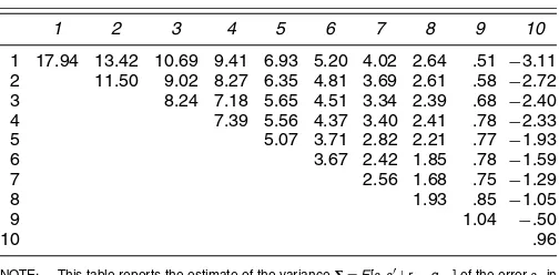
NOTE: This table reports the estimate of the variance=E[εtε′t|rM,t,qM,t] of the errorεtin the quadratic market model
rt=α+βrM,t+γqM,t+εt, t=1, . . . ,T,
wherert=Rt−RF,tι,rM,t=RM,t−RF,t, andqM,t=R2M,t−RF,t.Rtis theN-vector of portfolios returns,RM,t(RF,t) is the market return (the risk-free return), andιis aN-vector of 1’s.
assumes the value ξTF∗=35.34, which is strongly significant at the 5% level, because its critical value isχ.205(10)=18.31. Finally, from Table 2, we also see that smaller portfolios are characterized by larger variances of the residual error terms.
We performed several specification tests of the functional form of the mean portfolios return in (1). First, we estimated a factor SUR model including also a cubic power of market re-turns,R3M,t−RF,t, as a factor in addition to the constant, market
excess returns, and market squared excess returns. The cubic factor was found to be not significant for all portfolios. Further-more, to test for more general forms of misspecifications in the mean, we performed the Ramsey (1969) reset test on each port-folio, including quadratic and cubic fitted values of (1) among the regressors. In this case, too, the null of correct specification of the quadratic market model was accepted for all portfolios in our tests.
From the standpoint of our analysis, one central result from Table 1 is that the coskewness coefficients are (significantly) different from 0 for all portfolios in our sample, except for two of moderate size. Furthermore, coskewness coefficients tend to be correlated with size, with small portfolios having nega-tive coskewness with the market and the largest portfolios hav-ing positive market coskewness. This result is consistent with the findings of Harvey and Siddique (2000). It is worth noting that the dependence between portfolios returns and market re-turns deviates from that of a linear specification (as assumed in the market model), generating smaller (larger) returns for small (large) portfolios when the market has a large absolute return. This finding has important consequences for the assess-ment of risk in various portfolio classes; small firm portfolios, having negative market coskewness, are exposed to a source of risk additional to market risk, related to the occurrence of large absolute market returns. In addition, as we have already seen, market model (2), when tested against quadratic market model (1), is rejected with a largely significant Wald statistic. In the light of our findings, we conclude that the extension of the return-generating process to include the squared market re-turn is valuable.
4.2.2 Restricted Equilibrium Models. We now investigate
market coskewness in the context of models that are consis-tent with arbitrage pricing. To this end, we consider constrained
Table 3. PML Estimates of Model (6)
Portfolio i βi γi
1 1.106 −.017
(24.50) (−3.25)
2 1.191 −.012
(32.97) (−2.99)
3 1.186 −.009
(38.79) (−2.74)
4 1.170 −.009
(40.41) (−2.90)
5 1.140 −.009
(47.38) (−3.14)
6 1.112 −.006
(54.56) (−2.50)
7 1.107 −.001
(65.07) (−.76)
8 1.085 −.001
(73.37) (−.05)
9 1.017 .002
(93.66) (2.14)
10 .933 .003
(89.53) (2.63)
ϑ= −14.955 λ2=4.850
(−2.23) (.70)
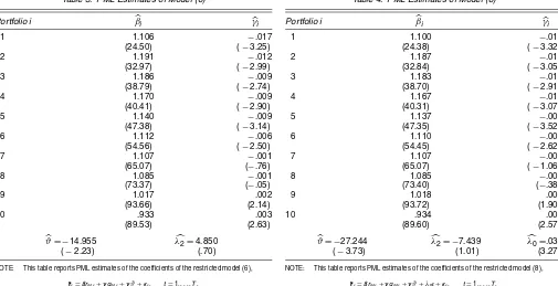
NOTE: This table reports PML estimates of the coefficients of the restricted model (6),
rt=βrM,t+γqM,t+γϑ+εt, t=1, . . . ,T,
whereϑis a scalar parameter, derived from the quadratic market model (1) by imposing the restriction given by the asset pricing model with coskewness,E(rt)=λ1β+λ2γ. The scalarϑ
and the premium for coskewnessλ2are related byϑ=λ2−E(qM,t). The restricted model (6) corresponds to hypothesisH1:∃ϑ:α=ϑγin (1).t-statistics are reported in parentheses.
PML estimation of models (6) and (8). Specification (6) is ob-tained from the quadratic market model after imposing restric-tions from the asset pricing model (4). Specification (8) instead allows for a homogeneous additional constant in expected ex-cess returns. The corresponding PML estimators are obtained from the algorithm based on (16)–(18), as reported in Sec-tion 3.3. The results for model (6) are reported in Table 3; those for model (8); in Table 4.
The point estimates and standard errors of parameters
β andγ are similar in the two models. Their values are close to those obtained from quadratic market model (1). In partic-ular, the estimates of parameter γ confirm that small (large) portfolios have significantly negative (positive) coskewness co-efficients. Parameterϑis significantly negative in both models, as expected, but the implied estimate for the risk premium for coskewness,λ2, is not statistically significant in either model. However, the estimate in model (8),λ2= −7.439, has at least the expected negative sign. Using this estimate, we deduce that for a portfolio with coskewnessγ = −.01 (a moderate-sized portfolio, such as portfolio 3 or 4), the coskewness contribution to the expected excess return on an annual percentage basis is approximately.9. This value increases to 1.5 for the smallest portfolio in our dataset.
We test the empirical validity of asset pricing model (4) in our sample by testing hypothesis H1 against the
alterna-tive,HF. The ALS test statistic ξT1 given in (21) assume the valueξT1=16.27, which is not significant at the 5% level, even though very close to the critical valueχ.205(9)=16.90. Thus there is some evidence that asset pricing model (4) may not be satisfied in our sample. In other words, an additional component other than covariance and coskewness to market may be present in expected excess returns. To test for the homogeneity of this
Table 4. PML Estimates of Model (8)
Portfolio i βi γi
1 1.100 −.017
(24.38) (−3.32)
2 1.187 −.012
(32.84) (−3.05)
3 1.183 −.010
(38.70) (−2.91)
4 1.167 −.010
(40.31) (−3.07)
5 1.137 −.009
(47.35) (−3.52)
6 1.110 −.006
(54.45) (−2.62)
7 1.107 −.002
(65.07) (−1.06)
8 1.085 −.001
(73.40) (−.38)
9 1.018 .002
(93.72) (1.90)
10 .934 .003
(89.60) (2.57)
ϑ= −27.244 λ2= −7.439 λ0=.032
(−3.73) (1.01) (3.27)
NOTE: This table reports PML estimates of the coefficients of the restricted model (8),
rt=βrM,t+γqM,t+γϑ+λ0ι+εt, t=1, . . . ,T,
whereϑandλ0are scalar parameters, derived from the quadratic market model (1) by imposing
the restrictionE(rt)=λ0ι+λ1β+λ2γ. Under this restriction, asset expected excess returns
con-tain a componentλ0that is not explained by either covariance or coskewness with the market.
The restricted model (8) corresponds to hypothesisH2:∃ϑ,λ0:α=ϑγ+λ0ιin (1).t-statistics
are reported in parentheses.
component across assets, we test hypothesisH2 againstHF.
The test statisticξT2in (22) assumes the valueξT2=5.32, well below the critical valueχ.205(8)=15.51. A more powerful test of asset pricing model (4) should be provided by testing hy-pothesisH1against the alternative,H2. This test is performed by the simplet-test of significance ofλ0. From Table 4, we see thatH1is quite clearly rejected. This confirms that asset pricing
model (4) may not be supported by our data. However, because
H2is not rejected, it follows that, if the additional component
unexplained by model (4) comes from an omitted factor, then its sensitivities should be homogeneous across portfolios in our sample. We conclude that size is unlikely to have explanatory power for expected excess returns when coskewness is taken into account. Moreover, the contribution to expected excess re-turns of the unexplained component, deduced from the estimate of parameterλ0, is quite modest, approximately.4 on a annual percentage basis. Note in particular that this is less than half the contribution due to coskewness for portfolios of modest size. As explained in Section 2.2,λ0>0 may be due to the use of a risk-free rate lower than the actual rate faced by investors.
4.2.3 Misspecification From Neglected Coskewness. As
already mentioned in Section 2, we are also interested in inves-tigating the consequences on asset pricing tests of erroneously neglecting coskewness. The results presented so far suggest that market model (2) is misspecified, because it does not take into account the quadratic market return. Indeed, when tested against quadratic market model (1), it is strongly rejected. For comparison, we report the estimates of parametersαandβ in market model (2) in Table 5. Theβ coefficients in Table 5 are close to those obtained in the quadratic market model reported in Table 1. Therefore, neglecting the quadratic market returns
Table 5. Estimates of Model (2)
Portfolio i αi βi
1 .080 1.102
(.39) (23.97)
2 .050 1.188
(.31) (32.34)
3 .092 1.183
(.67) (38.09)
4 .088 1.167
(.67) (39.65)
5 .148 1.135
(1.36) (46.43)
6 .044 1.110
(.48) (53.69)
7 .076 1.105
(1.00) (64.39)
8 .069 1.083
(1.05) (72.67)
9 .034 1.017
(.71) (92.41)
10 .005 .933
(.10) (88.18)
NOTE: This table reports for each portfolioi,i=1, . . . , 10, the PML–SUR estimates of the coefficientsαi,βiof the traditional market model
ri,t=αi+βirM,t+εi,t, t=1, . . . ,T,i=1, . . . ,N,
whereri,t=Ri,t−RF,tandrM,t=RM,t−RF,t.Ri,t is the return of portfolioiin montht, and RM,t(RF,t) is the market return (the risk-free return).t-statistics are reported in parentheses.
does not seem to have dramatic consequences for the estima-tion of parameterβ. However, we expect the consequences of this misspecification to be serious for inference. Indeed, we have seen earlier that the coskewness coefficients are correlated with size, with small portfolios having negative market coskew-ness and large portfolios having positive market coskewcoskew-ness. This feature suggests that size can have a spurious explanatory power in the cross-section of expected excess returns because it is a proxy for omitted coskewness. Therefore, as anticipated in Section 2, the ability of size to explain expected excess returns could be due to misspecification of models neglecting coskew-ness risk.
Finally, it is interesting to compare our findings with those reported by Barone Adesi (1985), whose investigation covers the period 1931–1975. We see that the sign of the premium for coskewness has not changed over time, with assets hav-ing negative coskewness commandhav-ing, not surprishav-ingly, higher expected returns. In contrast, both the sign of the premium for size and, consequently, the link between coskewness and size are inverted. Although it appears to be difficult to discrimi-nate statistically between a structural size effect and reward for coskewness, according to the criterion of Kan and Zhang (1999a,b) the size effect is more likely explained by neglected coskewness.
5. MONTE CARLO SIMULATIONS
In this section we report the results of a series of Monte Carlo simulations undertaken to assess the importance of spec-ifying the return-generating process to obtain reliably power-ful statistical tests. We compare the finite-sample properties (size and power) of two statistics for testing the asset pric-ing model with coskewness (4): the ALS statistic ξT1 in (21), which tests model (4) by the restrictions imposed on the return-generating process (1), and a GMM test statisticξTGMM, which
tests model (4) through the orthogonality conditions (9). In addition, we investigate the effects on the ALS statisticξT1 in-duced by the nonnormality of errorsεt or by the
misspecifica-tion of the return-generating process (1).
5.1 Experiment 1
The data-generating process used in experiment 1 is given by
rt=α+βrM,t+γqM,t+εt, t=1, . . . ,450,
whererM,t=RM,t−RF,t, andqM,t=R2M,t−RF,t, with
RM,t∼iidN(µM, σM2),
εt∼iidN(0,), (εt)independent of(RM,t),
RF,t=RF,a constant,
and
α=ϑγ+λ0ι.
The values of the parameters are chosen to be equal to the esti-mates obtained in the empirical analysis reported in Section 4. Specifically,β andγ are the third and fourth columns in Ta-ble 1, matrix is taken from Table 2,ϑ= −14.995 from Ta-ble 3,µM=.52,σM=4.41, andRF=.4, corresponding to the
average of the risk-free return in our dataset. Different values of parameterλ0 are used in the simulations. We refer to this data-generating process as DGP1. Under DGP1, whenλ0=0, quadratic equilibrium model (4) is satisfied. Whenλ0=0, equi-librium model (4) is not correctly specified, and the misspec-ification is in the form of an additional component, which is homogeneous across portfolios, corresponding to model (8). However, for any value ofλ0, quadratic market model (1) is well specified.
We perform a Monte Carlo simulation (10,000 replications) for different values ofλ0and report the rejection frequencies of the two test statistics,ξT1andξTGMM, at the nominal size of.05 in Table 6. The second row,λ0=0, reports the empirical test sizes. Both statistics control size quite well in finite samples, at least for sample sizeT=450. The subsequent rows, corresponding toλ0=0, report the power of the two test statistics against alter-natives corresponding to unexplained components in expected excess returns, which are homogeneous across portfolios. Note that such additional components, withλ0=.033, were found in the empirical analysis reported in Section 4. Table 6 shows that the power of the ALS statistic ξT1 is considerably higher than that of the GMM statisticξTGMM. This is due to the fact that the ALS statisticξT1use a well-specified alternative given by (1), whereas the alternative for the GMM statisticξTGMMis left unspecified.
5.2 Experiment 2
Under DGP1, residualsεt are normal. When residualsεtare
not normal, the alternative used by the ALS statisticsξT1[i.e., model (1)] is still correctly specified, because PML estimators are used to constructξT1. However, these estimators are not ef-ficient. In experiment 2 we investigate the effect of nonnormal-ity of residualsεton the ALS test statistic. The data-generating
process used in this experiment, called DGP2, is equal to DGP1
Table 6. Rejection Frequencies in Experiment 1
λ0 ξTGMM ξT1
0 .0404 .0559
.03 .0505 .4641
.06 .0712 .9746
.10 .1217 .9924
.15 .2307 .9945
NOTE: This table reports the rejection frequencies of the GMM statisticsξGMM
T [derived from (9)] and the ALS statisticsξ1
T[in (21)] for testing the asset pricing model with coskew-ness (4),
E(rt)=λ1β+λ2γ,
at the .05 confidence level, in experiment 1. The data-generating process (called DGP1) used in this experiment is given by
rt=α+βrM,t+γqM,t+εt, t=1, . . . , 450,
whererM,t=RM,t−RF,tandqM,t=R2M,t−RF,t, with
RM,t∼iidN(µM,σM2),
εt∼iidN(0,), (εt) independent of (RM,t),
RF,t=RF, a constant,
and
α=ϑγ+λ0ι.
Parametersβandγare the third and fourth columns in Table 1, the matrixis taken from Table 2,ϑ= −14.995 from Table 3,µM=.52,σM=4.41, andRF=.4, corresponding to the average of the risk-free return in our dataset. Under DGP1, whenλ0=0, the quadratic
equilib-rium model (4) is satisfied. Whenλ0=0, the equilibrium model (4) is not correctly specified, and
the misspecification is in the form of an additional component homogeneous across portfolios, corresponding to model (8).
but residualsεt follow a multivariatet-distribution with 5
de-grees of freedom. The correlation matrix is chosen so that the resulting variance of residuals εt is the same as under
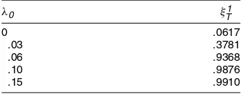
DGP1. The rejection frequencies of this Monte Carlo simula-tion (10,000 replicasimula-tions) for the ALS statisticξT1are reported in Table 7. The ALS statistic appears to be only slightly over-sized. As expected, power is reduced compared with the case of normality. However, the loss of power caused by nonnormality is limited. These results suggest that the ALS statistic does not suffer unduly from nonnormality of the residuals.
5.3 Experiment 3
In the Monte Carlo experiments conducted so far, the al-ternative used by the ALS statistic was well specified. In this last experiment, we investigate the effect of a misspecifica-tion in the alternative hypothesis in the form of condimisspecifica-tional
Table 7. Rejection Frequencies in Experiment 2
λ0 ξT1
0 .0617
.03 .3781
.06 .9368
.10 .9876
.15 .9910
NOTE: This table reports the rejection frequencies of the ALS statisticsξ1
T[in (21)] for testing (4), E(rt)=λ1β+λ2γ,
at the .05 confidence level, in experiment 2. The data-generating process used in this experiment (called DGP2) is the same as DGP1 (see Table 6), but the residualsεt follow a multivariate t-distribution with 5 degrees of freedom, and a correlation matrix such that the variance ofεtis the same as under DGP1.
Table 8. Rejection Frequencies in Experiment 3
λ0
ξT1under DGP4 (homoscedasticity)
ξT1under DGP3 (conditional heteroscedasticity)
0 .0587 .0539
.03 .3683 .1720
.06 .9333 .5791
.10 .9855 .9373
NOTE: This table reports the rejection frequencies of the ALS statisticsξ1
T[in (21)] for test-ing (4),
E(rt)=λ1β+λ2γ,
at the .05 confidence level, in experiment 3. In this experiment we consider two data-generating processes (called DGP3 and DGP4) having the same unconditional variance of the residualsεt, but such that the residualsεtare conditionally heteroscedastic in one case and homoscedastic in the other case. Specifically, DGP3 is the same as DGP1 (see Table 6), but the innovationsεt follow a conditionally normal, multivariate ARCH(1) process without cross-effects,
cov(εi,t, εj,t|εt−1)=
ωii+ρε2
i,t−1, i=j
ωij, i=j.
The matrix=[ωij] is chosen as in Table 2, andρ=.2. DGP4 is similar to DGP1 (see Table 6), with iid normal innovations whose unconditional variance matrix is the same as the unconditional variance ofεtin DGP3. Thus under DGP4, the alternative of the ALS statistics is well specified, but not under DGP3.
heteroscedasticity of errors εt. We thus consider two
data-generating processes having the same unconditional variance of the residualsεt, but so that the residualsεtare conditionally
heteroscedastic in one case and homoscedastic in the other case. Specifically, DGP3 is the same as DGP1, but innovations εt
follow a conditionally normal, multivariate ARCH(1)process without cross-effects,
covεi,t, εj,t
εt−1=
ωii+ρε2i,t−1, i=j
ωij, i=j.
Matrix= [ωij]is chosen as in Table 2, and ρ=.2. DGP4
is similar to DGP1, with iid normal innovations with the same unconditional variance matrix as innovationsεtin DGP3. Thus
under DGP4, but not under DGP3, the alternative of the ALS statistic is well specified. The rejection frequencies of the ALS statistic under DGP3 and DGP4 are reported in Table 8. The misspecification in the form of conditional heteroscedasticity has no effect on the empirical size of the statistics in these sim-ulations. The power of the ALS test statistic is reduced, but not drastically.
6. CONCLUSIONS
In this article we have considered market coskewness and investigated its implications for testing asset pricing models. By estimating a quadratic market model, which includes the market returns and the square of the market returns as the two factors, we showed that portfolios of small (large) firms have negative (positive) coskewness with market returns. This finding implies that small firm portfolios are exposed to a source of risk (i.e., market coskewness) that is different from the usual market beta and arises from negative covariance with large absolute market returns. We have shown that the coskewness coefficients of the portfolios in our sample are statistically significant. This finding rejects the usual market model and demonstrates the validity of the quadratic market model as a possible extension.
The analysis of the premium in expected excess returns in-duced by market coskewness requires the specification of ap-propriate asset pricing models including coskewness among the
rewarded factors. To obtain testing methodologies that are more powerful than a GMM approach, we tested asset pricing models including coskewness through the restrictions that they impose on the quadratic market model. We used asymptotic test sta-tistics whose finite-sample properties are validated by means of a series of Monte Carlo simulations. We found evidence of a component in expected excess returns that is not explained by either covariance or coskewness with the market. However, this unexplained component is relatively small and is consistent for instance with a minor misspecification of the risk-free rate. More important, the unexplained component is homogeneous across portfolios. This finding implies that additional variables, representing portfolios characteristics such as firm size, have no explanatory power for expected excess returns once coskewness is taken into account.
Finally, the homogeneity property of the unexplained compo-nent in expected excess returns is not satisfied when coskewness is neglected. Therefore, our results have important implications for testing methodologies, showing that neglecting coskewness risk can cause misleading inference. Indeed, because coskew-ness is positively correlated with size, a possible justification for the anomalous explanatory power of size in the cross-section of expected returns is that it is a proxy for omitted coskewness risk. This view is supported by the fact that the sign of the pre-mium for coskewness, contrary to that of size, has not changed in a very long time.
ACKNOWLEDGMENTS
The authors thank the participants in the 9th Conference on Panel Data, the 10th Annual Conference of the European Financial Management Association, the Conference on Mul-timoment Capital Asset Pricing Models and Related Topics, the INQUIRE UK 14th Annual Seminar on Beyond Mean-Variance: Do Higher Moments Matter?, the 2004 ASSA Meeting, and P. Balestra, S. Cain-Polli, J. Chen, C. R. Harvey, R. Jagannathan, R. Morck, M. Rockinger, T. Wansbeek, C. Zhang, two anonymous referees, and the editor, Eric Ghysels. All of them have contributed, through discussion, very help-ful comments and suggestions that improved this article. The usual disclaimer applies. Thanks are also due to K. French, R. Jagannathan, and R. Kan for providing their dataset. Swiss NCCR Finrisk is gratefully acknowledged by the first two authors.
APPENDIX A: RELATIONSHIP BETWEEN CROSS–MOMENT COSKEWNESS AND
THEγiPARAMETER
In this appendix we show how the parameter γi relates to
the coskewness term of our quadratic market model. We also report error estimates when the cross-moment coskewness is approximated by the parameterγi.
Our basic model is [see (1)]
rt,i=αi+βi(RM,t−RF,t)+γi(R2M,t−RF,t)+εi,t,
where
rt,i=Rt,i−RF,t.
The probabilistic measure of coskewness is defined by
cov(rt,i,R2M,t)=E[rt,iR2M,t] −E[rt,i]E[R2M,t],
which can be rewritten as
cov(rt,i,R2M,t)=βi
In the final equation, the first term is a measure of the mar-ket asymmetry, the second term is essentially our measure of coskewness, and the final term is equal to 0 by assump-tion (10). Evidently, our approach considers the second term only. However, our claim is motivated by the negligible effects of the first term. In fact, for valuesβi=1 andγi= −.01, which
are representative for small firm portfolios, the first term is.1, whereas the second is−15.Ifγi is equal to .003, as in large
firm portfolios, then the terms are equal to.1 and 4. Finally, if the portfolio has aγi=0, then the second term is also 0.
We are greatly indebted to one of the referees, whose com-ments highlighted this point.
APPENDIX B: PSEUDO–MAXIMUM LIKELIHOOD IN MODEL (8)
In this appendix we consider the PML estimator of model (8), defined by maximization of (15). We first derive the PML equa-tions. The score vector is given by
∂LT By equating the score to 0, we immediately find (16)–(18).
We now derive the asymptotic distribution of the PML esti-mator in model (8). Under usual regularity conditions (see the references in the main text), the asymptotic distribution of the general PML estimatorθdefined in (11) is given by
√
T(θ−θ0)−→d N(0,J−01I0J−01),
whereJ0(the so-called “information matrix”) andI0are sym-metric, positive-definite matrices defined by
J0= lim
We now compute matricesJ0andI0in model (8). The second derivatives of the pseudo-log-likelihood are given by
∂2LT
with the other ones vanishing in expectation. It follows that ma-tricesJ0andI0are given by [in the block representation corre-sponding to(β′,γ′, ϑ, λ0)′and vech()]
(All parameters are evaluated at true value). Therefore, the as-ymptotic variance–covariance matrix of the PML estimatorθin model (8) is given by
Vas[
(i.e.,J∗−0 1) does not depend on the distribution of error term εt, and in particular it coincides with the asymptotic variance–
covariance matrix of the ML estimator of (β′,γ′,ϑ ,λ0)′,
when εt is normal. In contrast, asymmetries and kurtosis
of the distribution of εt influence the asymptotic variance–
covariance matrix of vech()and the asymptotic covariance of(β′,γ′,ϑ ,λ0)′and vech(), through matricesSandK.
The asymptotic variance–covariance of(β′,γ′)′and(ϑ,λ0)′ is given explicitly in block form by
J∗−0 1=
Finally, we consider the asymptotic distribution of estimator λdefined in (19). The estimator
estimator on the extended pseudolikelihood
LT(θ,µ,f)
are asymptotically independent. It follows that
Vas[ √
T(λ2−λ2,0)] =f,22+Vas[
√
T(ϑ−ϑ0)].
APPENDIX C: ASYMPTOTIC LEAST SQUARES
In this appendix we derive the ALS statisticξT1 in (21) and
ξT2 in (22). In both cases the restrictions [see (20)] are of the form
It should be noted that exact tests (under normality) can be constructed for testing hypothesesH1andH2againstHF(see,
e.g., Zhou 1995; Velu and Zhou 1999). These tests are asymp-totically equivalent to the ALS tests used in this article for their computational simplicity. An evaluation of the finite-sample properties of the ALS test statistics is presented in Section 5.
[Received December 2002. Revised March 2004.]
REFERENCES
Banz, R. W. (1981), “The Relationship Between Return and Market Value of Common Stocks,”Journal of Financial Economics, 9, 3–18.
Barone Adesi, G. (1985), “Arbitrage Equilibrium With Skewed Asset Returns,”
Journal of Financial and Quantitative Analysis, 20, 299–313.
Barone Adesi, G., and Talwar, P. (1983), “Market Models and Heteroscedastic-ity of Residual SecurHeteroscedastic-ity Returns,”Journal of Business & Economic Statistics, 1, 163–168.
Black, F. (1972), “Capital Market Equilibrium With Restricted Borrowing,”
Journal of Business, 45, 444–455.
Bollerslev, T., and Wooldridge, J. M. (1992), “Quasi–Maximum Likelihood Estimation and Inference in Dynamic Models With Time-Varying Covari-ances,”Econometric Reviews, 11, 143–172.
Breeden, D. T. (1979), “An Intertemporal Asset Pricing Model With Sto-chastic Consumption and Investment Opportunities,”Journal of Financial Economics, 7, 265–296.
Campbell, J. Y., Lo, A. W., and MacKinlay, A. C. (1987),The Econometrics of Financial Markets, Princeton, NJ: Princeton University Press.
Chamberlain, G., and Rothschild, M. (1983), “Arbitrage, Factor Structure and Mean Variance Analysis in Large Asset Markets,”Econometrica, 51, 1281–1301.
Dittmar, R. F. (2002), “Nonlinear Pricing Kernels, Kurtosis Preference, and Evidence From the Cross-Section of Equity Returns,”Journal of Finance, 57, 368–403.
Engle, R. F., Hendry, D. F., and Richard, J. F. (1988), “Exogeneity,” Economet-rica, 51, 277–304.
Fama, E., and French, K. R. (1995), “Size and Book-to-Market Factors in Earn-ings and Returns,”Journal of Finance, 50, 131–155.
Gourieroux, C., and Jasiak, J. (2001),Financial Econometrics, Princeton, NJ: Princeton University Press.
Gourieroux, C., Monfort, A., and Trognon, A. (1984), “Pseudo-Maximum Likelihood Methods: Theory,”Econometrica, 52, 681–700.
(1985), “Moindres Carrés Asymptotiques,”Annales de l’INSEE, 58, 91–122.
Hansen, L. P. (1982), “Large-Sample Properties of Generalized Method-of-Moments Estimators,”Econometrica, 50, 1029–1054.
Hansen, L. P., and Jagannathan, R. (1997), “Assessing Specification Errors in Stochastic Discount Factor Models,”Journal of Finance, 52, 557–590. Harvey, C. R., and Siddique, A. (2000), “Conditional Skewness in Asset Pricing
Tests,”Journal of Finance, 55, 1263–1295.
Jagannathan, R., and Wang, Z. (1996), “The Conditional CAPM and the Cross-Section of Expected Returns,”Journal of Finance, 51, 3–53.
(2001), “Empirical Evaluation of Asset Pricing Models: A Comparison of the SDF and Beta Methods,” working paper, Northwestern University. Kan, R., and Zhang, C. (1999a), “GMM Test of Stochastic Discount
Fac-tor Models With Useless FacFac-tors,”Journal of Financial Economics, 54, 103–127.
(1999b), “Two-Pass Tests of Asset Pricing Models With Useless Fac-tors,”Journal of Finance, 54, 203–235.
Kan, R., and Zhou, G. (1999), “A Critique of the Stochastic Discount Factor Methodology,”Journal of Finance, 54, 1221–1248.
Kraus, A., and Litzenberger, R. (1976), “Skewness Preferences and the Valua-tion of Risk Assets,”Journal of Finance, 31, 1085–1100.
Lintner, J. (1965), “The Valuation of Risk Assets and the Selection of Risky Investments in Stock Portfolios and Capital Budgets,”Review of Economics and Statistics, 47, 13–37.
Merton, R. C. (1973), “An Intertemporal Capital Asset Pricing Model,”
Econometrica, 41, 867–887.
Newey, W. K., and West, K. D. (1989), “A Simple Positive Semi-Definite, Heteroscedasticity and Autocorrelation-Consistent Covariance Matrix,”
Econometrica, 55, 703–708.
Ramsey, J. B. (1969), “Tests for Specification Errors in Classical Linear Least Squares Regression Analysis,”Journal of the Royal Statistical Society, Ser. B, 31, 350–371.
Ross, S. A. (1976), “Arbitrage Theory of Capital Asset Pricing,”Journal of Economic Theory, 13, 341–360.
Rubinstein, M. E. (1973), “A Comparative Statics Analysis of Risk Premium,”
The Journal of Business, 46, 605–615.
Shanken, J. (1992), “On the Estimation of Beta Pricing Models,”Review of Financial Studies, 5, 1–33.
Sharpe, W. F. (1964), “Capital Asset Prices: A Theory of Market Equilibrium Under Conditions of Risk,”Journal of Finance, 40, 1189–1196.
Velu, R., and Zhou, G. (1999), “Testing Multi-Beta Asset Pricing Models,”
Journal of Empirical Finance, 6, 219–241.
White, H. (1981), “Maximum Likelihood Estimation of Misspecified Models,”
Econometrica, 50, 1–25.
Zellner, A. (1962), “An Efficient Method of Estimating Seemingly Unrelated Regressions and Tests for Aggregation Bias,”Journal of the American Sta-tistical Association, 57, 348–368.
Zhou, G. (1995), “Small-Sample Rank Tests With Applications to Asset Pricing,”Journal of Empirical Finance, 2, 71–93.