Evidence from Weather Shocks
Brian Jacob
Lars Lefgren
Enrico Moretti
a b s t r a c t
While the persistence of criminal activity is well documented, this may be due to persistence in the unobserved determinants of crime. There are good reasons to believe, however, that there may actually be a negative relationship between crime rates in a particular area due to temporal displacement. We exploit the correlation between weather and crime to examine the short-run dynamics of crime. Using variation in lagged crime rates due to weather shocks, we find that the positive serial correlation is reversed. These findings suggest that the long-run impact of temporary crime-prevention efforts may be smaller than the short-run effects.
I. Introduction
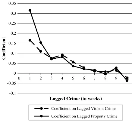
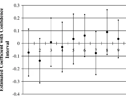
The persistence of criminal activity is well documented. Higher crime today in any particular area is associated with higher crime tomorrow. This serial correlation is illustrated in Figure 1. A 10 percent increase in violent crime in a typical city this week is associated with 1.6 percent more violence the following week, conditional on jurisdiction-year fixed effects. The serial correlation for property
Brian Jacob is assistant professor at the John F. Kennedy School of Government at Harvard University, Lars Lefgren is assistant professor of economics at Brigham Young University, and Enrico Moretti is associate professor of economics at the University of California at Berkeley. The authors thank Alberto Abadie, Dick Butler, Joe Doyle, Steve Levitt, Lance Lochner, Erzo Luttmer, Frank McIntyre, Bruce Sacerdote, two referees, and seminar participants at the 2004 NBER Summer Institute, BYU, Wisconsin, Florida, and 2004 AEA Meetings for useful suggestions. Email: Jacob can be contacted at brian_jacob@harvard.edu. Lefgren can be contacted at l-lefgren@byu.edu. Moretti can be contacted at moretti@econ.berkeley.edu. The data used in this article can be obtained beginning January 2008 through December 2010 from Enrico Moretti, 549 Evans Hall, Berkeley, CA 94720-3880, e-mail: Moretti@econ.berkeley.edu.
[Submitted February 2006; accepted October 2006]
ISSN 022-166X E-ISSN 1548-8004Ó2007 by the Board of Regents of the University of Wisconsin System
crime is even higher—10 percent more property crime this week is associated with over 3.1 percent more property crime the following week.1
One of the most common explanations for this autocorrelation is that potential offenders are influenced by the criminal behavior of others. In other words, a crime committed by one individual increases the likelihood that other individuals in the same locality will engage in criminal activity. In addition to social interactions that occur over a long time period through, for example, social learning, criminologists have long argued that forces such as imitation and revenge may lead to social mul-tiplier or contagion effects that operate over very short time horizons such as days or weeks.2However, the persistence in crime rates over time also could be explained by the persistence of unobserved factors that determine the costs and benefits of criminal activity such as police presence and poverty levels. Moreover, there are good reasons to believe that, particularly over a short time horizon, there actually may be anegative
relationship between crime rates in a particular area due to displacement—in other words, the shifting of criminal activity from one time or location to another. A study
Figure 1
The Persistence of Crime
Note: This figure shows the coefficient estimates from two separate regressions of current crime (vi-olent or property) on ten lags of crime (vi(vi-olent or property). The unit of observation is a jurisdiction-week. All crime rates are computed by dividing the actual number of crimes during a week by the average number of weekly crimes within the jurisdiction. Other covariates include jurisdiction fixed effects. Standard errors in parenthesis are clustered at the state*year*month level. Observations are weighted by the mean number of all crimes within the jurisdiction.
1. Correlation is positive for further lags. For example, a 10 percent increase in violent and property crime this week is associated with 1.1 and 1.6 percent higher crime two weeks later respectively.
of juvenile curfews in Detroit, for example, found that afternoon crime nearly dou-bled after the introduction of the curfew (Hesseling 1994).3
Understanding the dynamics of criminal activity is of interest for both practical and theoretical reasons. If thetimingof criminal behavior is more elastic to tempo-rary changes in the costs of crime than is the totalamountof criminal activity, then the effects of a police crackdown in a given week may be partially offset by increases in criminal activity in subsequent weeks. From a theoretical perspective, understand-ing the dynamics of criminal activity is important because it sheds light on the max-imizing behavior of criminals. Beginning with Becker (1968), economic models of criminal behavior have generally been constructed and tested using a static frame-work. While these models have been very useful in understanding some features of criminal behavior, they are not well suited to explaining how criminal behavior changes over time in response to changes in various costs and benefits. The economic literature on crime dynamics is limited.4
In this paper, we exploit the correlation between weather and crime to analyze the short-run dynamics of criminal activity. Our aim is to determine the true persistence of criminal activity by estimating the causal relationship between crime rates in dif-ferent time periods within the same locality. In other words, does more crime today lead to more or less crime tomorrow?
In order to eliminate any spurious serial correlation arising from persistent unob-served heterogeneity, we use an instrumental variable strategy that is based on weather shocks. Criminologists have long recognized that weather is strongly corre-lated with short-run fluctuations in crime, with hotter weather generally associated with more crime and inclement weather associated with less crime.5 Drawing on crime-level data from the FBI’s National Incident-Based Reporting System (NIBRS), we construct a panel of weekly crime data for 116 jurisdictions from 1995–2001. Simple OLS estimates confirm that violent and property crimes are highly correlated over time within localities. Weeks with above (below) average crime rates are typi-cally followed by weeks with above (below) average crime rates, even after control-ling for a rich set of jurisdiction-specific seasonality effects.
However, when we instrument for lagged crime with lagged weather conditions, we actually find theoppositeresult for both property and violent crime. The 2SLS estimates reveal that weeks with above average crime rates are followed by weeks withbelowaverage crime rates. Notably, our results do not appear to be driven by the persistence in weather conditions over time, or displacement of legal economic activity. Our models control for a series of jurisdiction-specific seasonality measures so that our identification essentially relies on deviations in expected weather patterns that influence crime rates in a particular locale.
The magnitude of the displacement is substantial. A 10 percent increase in violent crime due to a weather shock reduces violent criminal activity by about 2.6 percent 3. Similarly, prior work documents that juvenile violence peaks in the after-school hours on school days and in the evenings on nonschool days (Jacob and Lefgren 2003).
4. One notable exception is Lochner (1999).
in the following week. Moreover, there is evidence that additional displacement occurs over a longer time horizon. The estimated reduction in violent crime over a month is 5.4 percent, more than double the estimated displacement for one week. These findings are consistent with a model in which the marginal utility (cost) of vi-olence is decreasing (rising) in the amount of vivi-olence committed during the prior week. This would be true if, for example, an assailant who ‘‘settles a score’’ in one period feels less need to do so in a subsequent period.
The estimates for property crime are similar, though somewhat smaller. A 10 per-cent increase in property crime reduces property crime by about 2 perper-cent the follow-ing week. Interestfollow-ingly, while displacement of violent crime is apparent across multiple crime categories, displacement of property crimes is concentrated among crimes that involve highly valuable property, like car theft.6These results are consis-tent with a simple model in which transitory fluctuations in the costs of crime create an income effect that is manifested for multiple periods. This dynamic is similar to the one observed in a standard labor supply model with transitory shocks in the wage. Our findings suggest that criminal labor supply responds to transitory fluctuations in the wage in a manner that is similar to that of other self-employed individuals7and is also consistent with evidence on the presence of some forward-looking behavior of low-income populations.8At the same time, our findings are not consistent with the case of permanent-income offenders who face no liquidity constraints and have very long time horizon.
While we believe that these results provide interesting insight regarding the dy-namic optimization behavior of criminals, the relevance of our results for crime-prevention policy depends on the nature of the policy. Like all instrumental variable estimates, our findings reflect a particular local average treatment effect—namely, the impact of an exogenous increase in those crimes that are elastic to weather con-ditions. To the extent the changes in crime due to weather shocks are similar to changes induced by police interventions; our findings suggest that the long-run im-pact of short-term police crackdowns may be smaller than the initial effects of these policies.9
II. Simple Dynamic Models of Property
and Violent Crime
We present two simple models of property and violent crime. In these models, utility-maximizing criminals respond to transitory changes in the price of crime by shifting the time of their criminal activity, inducing a negative relationship between current and future crime. The goal of these models is to clarify the condi-tions under which temporal displacement may occur.
6. The value of property stolen also displays significant displacement: weeks where the value of stolen property is high are followed by weeks where the value is low.
7. See, for example, the studies of taxi drivers by Farber (2005) and Camerer, Babcock, Lowenstien, and Thaler (1997).
8. See studies of welfare recipients—for example, Grogger and Michalopoulos (2003).
A. Property Crime
Given the financial motivations underlying property crime, a standard labor supply framework provides considerable insight regarding the potential displacement of property crime. Displacement, if it occurs, would plausibly come about through an
income effect—in other words, a transitory increase in the benefits of crime generates a positive income effect which reduces the incentive to commit crime in subsequent periods. This suggests that displacement will not occur when individuals are unable to borrow and save. During lucrative periods, for example, nothing is saved so the next period’s choice of crime is unaffected. Likewise during lean times, offenders are unable to affect available income in subsequent periods by borrowing. This type of period-by-period maximization also would occur if individuals were completely myopic (Case 1). If, on the other extreme, criminals are farsighted and have access to good credit markets, there will also be no displacement because a transitory change in the price of criminal activity will have a negligible effect on lifetime in-come (Case 2). In order to generate a linkage between lagged and current criminal activity, it is necessary to construct a model that allows individuals to either save or borrow across periods. On the other hand, the credit market must be sufficiently imperfect or the time horizon must be short enough for a transitory shock in the ben-efits of criminal activity to have a meaningful income effect (Case 3).
We’ll now formalize this intuition in the context of a simple model. We assume that an individual’s utility each period is defined over consumption,c, and leisure,
l, in the following way:ut¼uðct;ltÞ. We will assume that uðct;ltÞ is increasing in both arguments and strictly concave. Each period a criminal must allocate a single unit of time between leisure and property crime,s. Because this time constraint must hold with equality, it must be the case thatlt¼12st. Each period, an individual earnswtstfrom criminal endeavors, wherewtis the net wage from criminal endeav-ors. Note thatwtreflects both the abundance of criminal opportunities and the period specific costs of engaging in criminal activity. In the context of our empirical anal-ysis, fluctuations in the weather generate variation inwt—perhaps due to weather-related changes in the supply of targets or in the disutility of committing crime outdoors.10
Case 1
The first case worth discussing is one in which individuals are unable or unwilling to save or borrow. In this case, the agent faces the following budget constraint:ct#wtst each period. We assume that the criminal maximizes discounted lifetime utility sub-ject to the budget constraints he faces. It is trivial to show that the first-order condi-tions are equivalent to those obtained from the period-by-period maximization problem. This is because each period’s utility and budget constraint is unaffected by that which has gone before or that which will occur later. For this reason, a tran-sitory shock to the benefit (wage) of property crime can have no impact beyond the current period.
Case 2
Another extreme case is that criminals are farsighted and have access to perfect cap-ital markets. While it is unlikely that most offenders have access to sophisticated capital markets, it still may be useful as a benchmark. Abstracting from uncertainty, each offender chooses a series of consumption and criminal activity to maximize his lifetime utility. The Lagrangian for the offender’s optimization problem is:
max
whereris the interest rate at which an offender can borrow or lend, andTis the num-ber of periods and is assumed to be large. In order to understand how a transitory change in the wage of crime affects subsequent criminal behavior, it is helpful to ex-amine the first-order conditions:
together with the budget constraint. Equations 2 and 3 must hold for allt. It is now no longer true that the first-order conditions are equivalent to those consistent with period-by-period optimization. Instead, the ability to borrow and save implies that the marginal utility of lifetime income,l, is a function of the wages of crime in every period. Thus, while an increase in wt can induce a substitution effect that causes st to rise, the only mechanism through which it can affectst+ 1 is throughl. This corresponds to an income effect. In dynamic models of labor supply, it is generally assumed that the lifetime income effects of a transitory wage shock are minimal— limiting the temporal displacement of property crime.
Case 3
Consider a model identical to the one above except withT¼2. For simplicity, assume that the discount rate and the interest rate are both zero, and the utility function is separable in consumption and leisure. Under these assumptions, the first-order con-ditions are identical to those in Equations 2 and 3. What happens to crime at Time 2 when there is an exogenous shock to the net benefit of committing crime in Period 1? The comparative statics are straightforward:
the benefits of crime generates a positive income effect (lowering the marginal utility of wealth), which reduces the incentive to commit crime in subsequent periods. As-suming that the substitution effect dominates the income effect in the first period,11a transitory increase in the wage of crime will initially lead to higher levels of crime and will then reduce subsequent criminal activity. In this case, we will observe tem-poral displacement of property crime.
Even in this third case, it is interesting to question what type of property crime would generate the strong income effects necessary to observe temporal displace-ment. Clearly, it is unlikely that stealing a small inexpensive item could have any significant income effect. If any displacement occurs, we should observe it only for crimes that involve goods with substantial monetary value. Notably, this is exactly what we observe in the data. We find that car theft is characterized bytotal
displacement, while all other property crimes are characterized by virtually no
displacement.
B. Violent Crime
While the motives underlying violent crime are less often financial, temporal dis-placement still may occur. In the framework outlined below, temporal disdis-placement may occur for two reasons. First, the benefits of violence may persist over time. This would be true if injuring an individual in the first period ‘‘settled a score’’ or ‘‘taught a lesson,’’ reducing the need to do so again in the second period. Second, the costs of violence in one period may depend on the level of violence in the previous period. For example, alcohol and/or drugs are sometimes a cofactor in violent crimes (bar fights, domestic violence, etc.). It is possible that the violence that was precipitated by substance use in the first period may cause the offender to feel guilty, taming al-cohol consumption in the second period. Alternatively, a violent act in the first period may result in arrest and/or greater police supervision in the second period.
Consider a simple two-period model. Assume that first-period utility is given by the following:
u1¼g1ðv1Þ2u1v1; ð5Þ
wherev1is violence in the first period,g1ðv1Þis an increasing but concave function ofv1, andu1is an exogenous per-unit cost of violence. Second-period utility is given by the following:
u2¼g2ðv2+dv1Þ2u2ðv1Þv2; ð6Þ
wherev2is violence in Period 2,dis the fraction of the benefits of violence that carry over to the next period, g2ðv2+dv1Þ is an increasing and concave function, and u2ðv1Þis the per-unit cost of committing violence in the second period.
11. If we thought of the amount of property crime as the dollars generated from criminal activity,wtst, the
In our model, the per-unit cost of violence in the second period,u2ðv1Þ, is an in-creasing and convex function of first-period violence. This assumption seems plau-sible.12 The criminal’s optimization problem involves choosing Periods 1 and 2 violence to maximize utility over the two periods. The first-order conditions of this problem are the following:
These conditions define the equilibrium level of crime in the two periods.13 What happens to violent crime if the cost of first-period violence exogenously increases (for example, because of a weather shock)? It is not surprising that that an increase in first-period violence results in a decrease in violent crime in the first period:dv1
du1,0.
14The comparative static for second-period crime is more relevant for our analysis. In particular, what happens to violent crime in Period 2 when there is an exogenous shift in the cost of violent crime in Period 1?
dv2
The denominator of Equation 9 must be positive in order for the second order con-ditions to hold. Both terms in the numerator are positive suggesting that second-period violence is likely to increase in the first-second-period cost of violence if either the benefits of violence are durable ðd.0Þ or the marginal cost of second-period vio-lence is rising in first-period viovio-lence. These findings suggest that the displacement of violent crime can occur under plausible conditions.
III. Empirical Strategy
The previous section suggests that crime in one period may affect crime in the next period either positively or negatively. The basic empirical frame-work therefore relies upon estimating the following simple equation:
crimei;t¼b0+b1crimei;t21+eit; ð10Þ
12. Violent acts in the first period may result in arrest or increased police supervision; injuries sustained in the first period could hamper the ability to commit violent crime in the second period; or, for crimes such as domestic violence, it is possible that guilt over a violent act in Period 1 would increase the cost of com-mitting a similar act in Period 2.
13. Note that these conditions take into account thatg2ðv2+dv1Þ
wherecrimei;treflects the level of crime in jurisdictioniin periodtandb1 reflects the causal effect of an exogenous increase in criminal activity on the next period’s crime. Following the models presented in Section II,b1 is the net effect of social interactions and displacement. The empirical challenge is thatcrimei;t21 is almost certainly positively correlated to the error termeit, since factors affecting the costs and benefits of crime are likely persistent over time.
The ideal instrumental variable is correlated with criminal activity in periodt-1 but uncorrelated to the error term. One candidate instrument is the weather. The corre-lation between criminal activity and weather conditions has been well documented.15 It has been hypothesized that higher temperatures might increase aggression directly (see Anderson 2001), thus providing a transitory increase in the net benefit of crim-inal activity. Adverse weather conditions may affect the cost of executing a particular crime, due to changes in the ease of transportation or the likelihood of witnesses to the crime, which may influence the chance of arrest.
In this model, the structural equation is given by:
crimeit¼BXit+b1crimei;t21+b2weatherit+eit ð11Þ
whereiindexes jurisdictions, and tindexes time period (in our analysis, a week),
weatherit is a vector of weather variables, and the vector Xit includes jurisdiction *year fixed effects, jurisdiction-specific fourth order polynomials in day-of-year and fixed effects for each month. The first stage is given by:
crimei;t21¼GXit+g1weatheri;t21+g2weatherit+hit:16 ð12Þ
To increase the efficiency of our estimates, we weight each observation by the av-erage number of (violent or property) crimes committed each week within the juris-diction.17The standard errors are cluster corrected at the state*year*month level as weather and criminal activity may be spatially and temporally correlated. In some models we include more than one lag in crime. When Equation 11 includes crime at t-1, t-2, t-3, andt-4, we instrument t-2 crime usingt-2 weather conditions, t-3 crime usingt-3 weather conditions, and so forth.
The key identifying assumption in this model is that, conditional on weather at timet and other covariates, weather at timet-1 cannot directly influence crime at timet. More formally, covðeit;weatheri;t21jweatherit;XitÞ ¼0. In assessing this
as-sumption, it is important to highlight several potential issues. A first concern is that weather, when measured at high frequency, is serially correlated. Therefore, in the
15. See Cohn’s (1990) extensive literature review on the subject. More recent work on the issue by Rotton and Cohn (2000) and Field (1992) confirms the finding.
16. One might be concerned that this instrumenting strategy does not work because the first stage seems inconsistent with the recursive structure of the data-generating process. However, it is trivial to show that, if the exclusion restriction holds, our strategy yields an unbiased estimate ofb1.
17. To understand why we do this, suppose that criminal activity is generated by a Poisson process, the mean and variance or crime with a jurisdiction both equalci. We discuss below that we normalize crime
rates by the mean weekly incidence over the sample—doing so yields point estimates that can be inter-preted as percentage effects. In this case, the variance of the normalized crime measure is 1=ci. By
weight-ing each jurisdiction byci, which is the approximate inverse of the variance of its residual, we increase the
absence of good controls for current weather, lagged weather may be directly cor-related with current crime because it will contain information regarding current weather. While we do control for current weather conditions in our models, it is pos-sible that weather within a period is measured imperfectly, in which case lagged weather still may provide information regarding the unobserved aspects of current weather. For example, one day’s maximum temperature likely provides informa-tion regarding the weather condiinforma-tions at 1 a.m. of the next day. The combinainforma-tion of serial correlation in weather, along with imperfect measures of weather conditions in any one period, will violate the assumptions necessary for satisfactory identifica-tion and result in apositivebias in the coefficient on lagged crime. We can show that this bias decreases as the length of the time window expands. (For a formal proof, see Appendix A in Jacob, Lefgren, and Moretti 2004.) Additionally, we later show the results of a ‘‘reverse experiment’’ in which we estimate the effect of futurecrime on current crime, and instrument for future crime with future weather. The instru-ment coefficient on future crime is insignificant, suggesting that this type of bias in insignificant.
A second concern is that weather may lead to the displacement of noncriminal economic activity. To the extent that criminal activity is follows noncriminal eco-nomic activity, apparent displacement of criminal activity may not generalize to set-tings in which noncriminal activity remains constant. To assess whether empirically this is an important source of bias, we examine three pieces of evidence, all of which are discussed in detail in Section VI. First, we provide evidence that some noncrim-inal activities—namely, traffic patterns—are not significantly displaced by weather conditions. Second, we compare the impact of lagged crime on indoor and outdoor crimes separately. Third, we explore whether the relationship between the victim and offender of violent crime is associated with the magnitude of displacement. Taken together, these three pieces of evidence indicate that our finding of temporal dis-placement is unlikely to be driven only by noncriminal economic activity.
Finally, in interpreting our estimates it is important to realize that our strategy yields a particular local average treatment effect, LATE (Imbens and Angrist 1994). The estimates presented here reflect the impact of an exogenous increase in those crimes that are elastic to weather conditions. We will provide evidence in Section VI that weather affects a broad range of criminal behaviors. It is possible, however, that the set of criminals whose behavior is affected by the weather is different from the set of criminals who vary their behavior in response to transitory law enforcement activity. Thus, our findings might not fully generalize to other contexts.
IV. Data
The massive detail of the database allows us to aggregate data into categories and time periods of our choosing. Unfortunately, many of the largest jurisdictions do not to participate in NIBRS. The 2001 data file contains information on over three million incidents reported in 3,611 different jurisdictions including Austin, Texas, and Cincinnati, Ohio. Most jurisdictions in the sample, however, are very small with more than 70 percent reporting fewer than 500 crimes for the whole year. Earlier sample years contain information on even fewer jurisdictions.
Because the most severe crimes occur infrequently in the jurisdictions that we ob-serve, we focus our analysis on broad aggregates such as violent and property crime. Violent crimes include simple and aggravated assault, intimidation, homicide, man-slaughter, and sex crimes. Property crimes include extortion, counterfeiting, fraud, larceny, vehicle theft, robbery, and stolen property offenses.18Data on weather are from the National Climatic Data Center (NCDC). They contain daily readings of minimum and maximum temperature, and inches of precipitation for 24,833 weather stations in the United States. We average these weather measures across stations within each county to construct a county-level panel of daily weather conditions.
As discussed in Section IV, we aggregate the daily data for both crime and weather to the weekly level in order to reduce any bias due to the autocorrelation of weather.19 Our primary analysis sample includes 116 jurisdictions for the period 1995–2001 with a total of 26,338 jurisdiction-week observations. In order to maxi-mize the statistical power of our estimates, we have chosen the largest jurisdictions for which NIBRS data is available. While NIBRS is by no means a nationally rep-resentative sample of police jurisdictions in the United States, and the largest juris-dictions in the country tend not to participate, our sample does include a relatively diverse set of cities and counties. (For a complete list of the jurisdictions included in our sample, see Table 6.)20
Because some jurisdictions are larger than others, it is helpful to normalize the crime rate across jurisdictions to reduce heteroskedasticity. This specification also allows weather to have the same percentageeffect on the crime rate—regardless of jurisdiction size. Researchers often address these concerns by using the natural log of the crime rate. This specification is not well suited for the current paper be-cause, when examining specific types of crimes, it is sometimes the case that no 18. Robbery is included as a property crime because the underlying motive is financial. Vandalism is ex-cluded for the same reason.
19. In some jurisdictions, multiple weeks in a single month contain no criminal activity due to misreporting by the police agency. In these cases, we restrict the sample in following manner. We drop jurisdiction-month observations in which the jurisdiction-monthly crime rate is more than twice the jurisdiction-specific interquar-tile range below the median. We use the monthly crime rate because in some jurisdictions, it might be the case that no crime occurred over several days or weeks. By using a longer time period, we are more con-fident that we are excluding observations with gross underreporting. We choose to restrict the sample on the basis of median and interquartile range because these measures are less sensitive to periodic massive under-reporting than are the mean and standard deviation. However, if monthly crime is normally distributed, our exclusion restriction corresponds to months in which criminal activity is more than 2.67 standard deviations below the mean.
crimes of a particular type occur during the course of a given week. Our large sample size and massive number of covariates complicate the use of count models. Thus, in our primary specifications our measure of criminal activity is the number of crimes committed during the week divided by the average weekly incidence in the jurisdic-tion during the sample period.
In our sample, the mean weekly temperature in our sample is 58 degrees Fahren-heit. In the average week, there is only 0.11 inches of daily precipitation. In the 18 percent of weeks that experience some snowfall, there is an average of 0.40 daily inches of snowfall. Note that a number of jurisdictions appeared to be somewhat in-consistent in reporting snowfall. For this reason, we include only measures of tem-perature and precipitation in our preferred specifications, though our estimates are robust to the inclusion and use of snowfall.
V. Empirical Findings
A. Graphical Relationship between Lagged and Current Crime
Figures 2a and 2b illustrate the baseline serial correlation of crime in our data. To do so, we regress the violent or property crime rate in Periodton ten lags of crime within
Figure 2a
The Estimated Relationship between Current and Lagged Violent Crime
the same jurisdiction, controlling for the same set of covariates that will be used in our primary estimation—namely, jurisdiction*year fixed effects, jurisdiction-specific fourth order polynomials in day of year as a smooth control for seasonality, month fixed effects, and average temperature and total precipitation in Periodtas controls for current weather conditions. Standard errors are clustered by state-year-month to account for spatial and temporal correlation. The figures present the coefficients on all lagged crime variables. Figures 2a and 2b differ from Figure 1 in that it includes a detailed set of controls.21
The top panel shows that violence during each of the past five weeks is a statisti-cally significant predictor of violence in the current period. The coefficients on the lags start at 0.065 and generally fall with distance from the reference week. By Week 6, the coefficients are statistically insignificant. In the bottom panel, we see that the
Figure 2b
The Estimated Relationship between Current and Lagged Property Crime
Notes: Each panel figure shows the coefficient estimates from a regression of current property crime on 10 lags of property crime. The unit of observation is a jurisdiction-week. All crime rates are com-puted by dividing the actual number of crimes during a week by the average number of weekly crimes within the jurisdiction. Other covariates include average temperature and total precipita-tion in the current period; jurisdicprecipita-tion-year fixed effects, jurisdicprecipita-tion-specific fourth order polyno-mials in day-of-year, and fixed effects for month. Standard errors in parenthesis are clustered at the state*year*month level. Observations are weighted by the mean number of all crimes within the jurisdiction.
serial correlation for property crime is even higher than that for violent crime (for example, the coefficient on the first lag is 0.22), but the autocorrelation appears to decay in a similar way. While these conditional correlations are statistically signif-icant, it is interesting to note that they are smaller than the unconditional correlations presented in Figure 1. This suggests that factors associated with jurisdiction-specific time and jurisdiction-specific seasonality effects (for example, factors such as sea-sonal changes in the economy, or police interventions) have a strong influence on crime rates.
B. The Effect of Weather on Crime
Table 1 examines the relationship between weather and violent as well as property crime using the baseline set of controls described above. The dependent variable here is the number of incidents in a jurisdiction-week divided by the average number of weekly incidents in that jurisdiction over the entire sample period, so that the coefficients on the explanatory variables can be interpreted roughly as a percent change in the outcome. Looking first at Column 1, we see that weather—particularly temperature—is strongly correlated with violent crime. A ten degree increase in the average weekly temperature is correlated with about a 5 percent increase in violent criminal activity. Precipitation, on the other hand, is associated with reductions in criminal activity. An increase in average weekly precipitation of one inch is associ-ated with a 10 percent reduction in violence. These effects are highly statistically significant—theF-statistic of joint significance is over 200.22
We see similar patterns for property crime, although weather appears to be less predictive of property than violent crime. As the average weekly temperature rises by 10 degrees, property crimes fall by about 3 percent. The coefficient on precipita-tion is not statistically significant. TheF-statistic of joint significance for all weather variables is 51.
Columns 2–10 show the effect of temperature and precipitation on a variety of dif-ferent types of crimes. This not only provides additional insight regarding the overall weather-crime relationship but, perhaps more importantly, allows one to better inter-pret the local average treatment effect of the estimates presented below. The results indicate that the effect of weather is quite consistent across all types of violent crime. Weather has a similar effect on domestic violence and violence against strangers; across crimes of varying levels of seriousness; regardless of whether a weapon was used; and for violent crimes involving juvenile as well as adult offenders. The results for various types of property crimes are roughly similar—higher temperature is always associated with more property crime—although the effect of precipitation varies more for property than violent crime.23
22. There is a convex relationship between temperature and crime—very hot temperatures result in a more than proportional increase in violence—but a concave relationship between precipitation and violence. (See Table 3 in Jacob, Lefgren, and Moretti 2004.)
Panel A: Violent Crime
Temperature/100 0.478** 0.494** 0.633** 0.313** 0.434** 0.649** 0.569** 0.449** 0.416** 0.541**
(0.028) (0.032) (0.062) (0.050) (0.032) (0.054) (0.061) (0.033) (0.180) (0.071)
Precipitation 20.097** 20.089** 20.171** 20.046** 20.094** 20.109** 20.141** 20.090** 20.120** 20.157**
(0.009) (0.011) (0.020) (0.016) (0.010) (0.017) (0.018) (0.010) (0.051) (0.025)
F-statistic 203.5 148.01 85.47 25.85 138.00 96.84 80.72 137.86 5.26 46.1
[0.00] [0.00] [0.00] [0.00] [0.00] [0.00] [0.00] [0.00] [0.00] [0.00]
Rsquared 0.47 0.40 0.20 0.29 0.45 0.26 0.27 0.42 0.05 0.223
Panel B: Property Crime
Temperature/100 0.292** 0.313** 0.049 0.386** 0.190** 0.499** 0.161**
(0.024) (0.027) (0.054) (0.044) (0.053) (0.095) (0.042)
Table 1 (continued)
Panel B: Property Crime
All
Property Larceny Shoplifting Burglary
Vehicle
Theft Robbery
Property Value
(1) (2) (3) (4) (5) (6) (7)
Precipitation 20.008 20.020** 0.035* 0.034** 0.007 0.033 0.002
(0.008) (0.010) (0.019) (0.014) (0.023) (0.031) (0.014)
F-statistic 51.24 49.50 5.00 26.61 4.26 7.89 7.44
[0.00] [0.00] [0.00] [0.00] [0.00] [0.00] [0.00]
Rsquared 0.593 0.545 0.261 0.335 0.241 0.097 0.313
Notes: The unit of observation is a jurisdiction-week and the number of observations is 26,567. All crime rates are computed by dividing the actual number of crimes during a week by the average number of weekly crimes within the jurisdiction. All models include jurisdiction-year fixed effects, jurisdiction-specific fourth order polynomials in day-of-year, and fixed effects for month. Standard errors are in parentheses.P-values are contained in brackets. Standard errors are clustered at the state*year*month level to take into account the correlation across jurisdictions within a state and within a jurisdiction over time. All weather variables are weekly aver-ages. Precipitation is measured in inches. Property value indicates the total monetary value (in dollars) of stolen property in that jurisdiction-week. Observations are weighted by the mean number of all crimes within the jurisdiction. * statistically significant at the 10 percent level; ** statistically significant at the 5 percent level.
The
Journal
of
Human
C. The Effect of Heat Waves on Crime
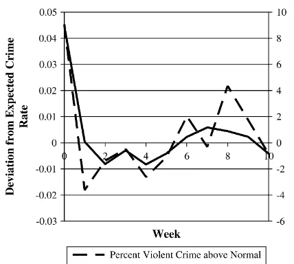
Here we illustrate the intuition behind our instrumental variable strategy using an ex-ample of extreme weather conditions—heat waves. We identify a set of unusually hot weeks that were followed by relatively normal weather.24If displacement occurs, we should see relatively high crime during the hot week and relatively low crime during the subsequent weeks.
Figure 3a shows the results for violent crime. The solid line shows average tem-perature during the hot week (Time 0) along with the temtem-perature during the subse-quent ten weeks. The dashed line shows how the average deviation of the violent crime rate from the predicted rate. In Week 0, both temperatureand violent crime are higher than expected. Indeed, the violent crime rate is 4.5 percentage points higher than normal. The following week, temperature is close to its predicted value.
Figure 3a
Heat Waves and Violent Crime
Notes: For each panel, we regressed temperature on month fixed effects, jurisdiction*year fixed effects and jurisdiction-specific fourth order polynomials in day of year. We included periods in our sample in which the temperature in week 0 was more than 6 degrees Fahrenheit above predicted (using our controls) and the temperature in Week 1 was within 3 degrees of predicted. For each week, we show the average temperature residual—weighting each jurisdiction by the average number of crimes committed during a week. We also show the average violent crime residual, which is obtained by running a regressions with controls discussed above.
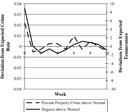
Violent crime, however, is nearly 2 percentage pointslowerthan normal, suggesting displacement of about 40 percent over the subsequent week. Over the next ten weeks, both temperature and the rate of violent crime bounce around the predicted level, though violent crime is unusually high eight weeks after the hot week. Figure 3b shows the analogous results for property crime. During the initial hot week, property crime is more than 2 percentage points higher than expected. The following week it is about 0.5 percentage points lower. This is again consistent with displacement, though the drop in Week 1 is smaller than for violent crime. In the subsequent weeks, we again see a small amount of variation around the predicted crime rate.
D. IV Estimates of the Impact of Lagged Crime on
Current Criminal Activity
The analysis of heat waves—an extreme weather shock—casts doubt on thepositiveserial correlation of crime that one observes in the raw data. Indeed, these results indicate that, over a short-time horizon, exogenous increases in crime
Figure 3b
Heat Waves and Property Crime
may be followed bydecreasesin crime—suggesting temporal displacement in criminal activity. To more formally examine this for the full data sample, Tables 2 and 3 pre-sent OLS and IV estimates of the relationship between lagged and current crime. By way of reminder, the first and second stage specifications are given by Equations 11 and 12 respectively. As explained above, all models include jurisdiction*year fixed effects, month effects and the jurisdiction-specific fourth-order polynomials in day-of-year to control for seasonality. In order to account for the persistence of weather over time, they also control forcurrent weather conditions including the weekly average of daily mean temperature, inches of precipitation. Our instruments are lagged average temperature and total precipitation.25To take into account that the error terms are not independent across jurisdictions or over time, we cluster the stan-dard errors at the state*year*month level.26
Looking first at the violent crime results in Table 2, the OLS estimates show the strong positive correlation documented in Figures 2a and 2b. However, when we in-strument for lagged violent crime using lagged weather conditions, the results are actuallyreversed. The IV estimate in Column 2, for example, indicates that a 10 per-cent increase in criminal activity in one week is associated with a 2.6 perper-cent de-creasethe following week. Note that the first stage F-statistic is 213, indicating that our instruments are quite strong (which is also reflected in the precision of our estimates). In Columns 4, 6, and 8, we see that the effects of more distant lags are generally smaller than the first lag, though most estimates remain statistically sig-nificant and negative. The sum of the lags provides a measure of the total displace-ment over an extended period of time. For example, in Column 8, the sum of the four lags is -0.536, indicating that a 10 percent increase in violent crime during a partic-ular week is associated with a reduction of roughly 5.4 percent over a one-month period—roughly double our estimate for the one-week period. Note that the magni-tude of the implied displacement is quite large. For example, these results suggest that the actual impact of a violent crime-prevention program is less than halfthe magnitude of its contemporaneous impact. Note that these results are statistically significantly different from zero as well as one (which would indicate complete dis-placement).
The results for property crime in Table 3 reveal a similar pattern. In stark contrast to the positive correlations documented in OLS, the IV estimates suggest that lagged crime has a statistically significantnegativeeffect on crime in the current period. The estimate in Column 2, for example, indicates that a 10 percent increase in property crime in one week will lead to a 2.0 percent decline in property crime the follow-ing week. Note that, like in violent crime, the IV estimates are not only statistically significantly different than zero, but also statistically significantly different from the OLS estimates. In all models, the sum of the lags is negative and statistically
25. We do not use snowfall due to concerns about the consistency of data collection. Our estimates are robust to the inclusion of snowfall measures.
Table 2
OLS and IV Estimates of the Relationship between Current and Lagged Violent Crime
Dependent Variable: Violent Crime in Periodt
OLS IV OLS IV OLS IV OLS IV
(1) (2) (3) (4) (5) (6) (7) (8)
Crimet-1 0.083** 20.260** 0.077** 20.209** 0.072** 20.215** 0.068** 20.221** (0.010) (0.054) (0.009) (0.050) (0.009) (0.049) (0.008) (0.050) Crimet-2 — — 0.052** 20.172** 0.047** 20.159** 0.043** 20.159**
(0.008) (0.052) (0.008) (0.045) (0.008) (0.047)
Crimet-3 — — — — 0.032** 20.070 0.026** 20.049
(0.008) (0.052) (0.008) (0.047)
Crimet-4 — — — — — — 0.049** 20.105**
(0.008) (0.054)
The
Journal
of
Human
F-Statistic—first stage [p-value]
— 213.58 — 112.5-113.0 — 81.1-78.3 — 59.9-66.0 [0.00] [0.00-0.00] [0.00-0.00] [0.00-0.00] Observations 26,338 26,338 25,929 25,929 25,893 25,893 25,853 25,853
Periodtweather Yes Yes Yes Yes Yes Yes Yes Yes
Jurisdiction*year effects Yes Yes Yes Yes Yes Yes Yes Yes
Month effects Yes Yes Yes Yes Yes Yes Yes Yes
Jurisdiction-specific fourth order polynomial in day of year
Yes Yes Yes Yes Yes Yes Yes Yes
Notes: The unit of observation is a jurisdiction-week. The number of observations varies depending on the number of lags included. All crime rates are computed by dividing the actual number of crimes during a week by the average number of weekly crimes within the jurisdiction. Standard errors are in parenthesis. Standard errors are clustered at the state*year*month level to take into account the correlation across jurisdictions within a state and within a jurisdiction over time.P-values for the
F-statistics are shown in brackets. For models with multiple instruments, minimum and maximumF-statistic andp-value are shown. Observations are weighted by the mean number of all crimes within the jurisdiction. * statistically significant at the 10 percent level; ** statistically significant at the 5 percent level.
Jacob,
Lefgren,
and
Moretti
Table 3
OLS and IV Estimates of the Relationship between Current and Lagged Property Crime
Dependent Variable: Property Crime in Periodt
OLS IV OLS IV OLS IV OLS IV
(1) (2) (3) (4) (5) (6) (7) (8)
Crimet-1 0.279** 20.201** 0.241** 20.171** 0.233** 20.176** 0.229** 20.172** (0.012) (0.083) (0.010) (0.080) (0.010) (0.084) (0.010) (0.084) Crimet-2 — — 0.127** 20.136* 0.112** 20.138* 0.104** 20.149*
(0.008) (0.090) (0.008) (0.083) (0.007) (0.084)
Crimet-3 — — — — 0.054** 20.011 0.040** 20.016
(0.008) (0.083) (0.007) (0.084)
Crimet-4 — — — — — — 0.056** 20.010
(0.008) (0.096) Sum of coefficients 0.279** 20.201** 0.368** 20.307** 0.399** 20.325** 0.429** 20.326*
(0.012) (0.083) (0.014) (0.116) (0.015) (0.137) (0.016) (0.204)
The
Journal
of
Human
Observations 26,338 26,338 25,929 25,929 25,893 25,893 25,853 25,853
Periodtweather Yes Yes Yes Yes Yes Yes Yes Yes
Jurisdiction*year effects Yes Yes Yes Yes Yes Yes Yes Yes
Month effects Yes Yes Yes Yes Yes Yes Yes Yes
Jurisdiction-specific fourth order polynomial in day of year
Yes Yes Yes Yes Yes Yes Yes Yes
Notes: The unit of observation is a jurisdiction-week. The number of observations varies depending on the number of lags included. All crime rates are computed by dividing the actual number of crimes during a week by the average number of weekly crimes within the jurisdiction. Standard errors are in parenthesis. Standard errors are clustered at the state*year*month level to take into account the correlation across jurisdictions within a state and within a jurisdiction over time.P-values for the
F-statistics are shown in brackets. For models with multiple instruments, minimum and maximumF-statistic andp-value are shown. Observations are weighted by the mean number of all crimes within the jurisdiction. * statistically significant at the 10 percent level; ** statistically significant at the 5 percent level.
Jacob,
Lefgren,
and
Moretti
significantly different than both zero and one. The effects are somewhat smaller for property than violent crime, but are still substantial. In Column 8, the sum of the four lagged crime measures is20.33, which implies that for property crime, the displace-ment that occurs over one month is roughly 50 percent more than that which occurs over one week.
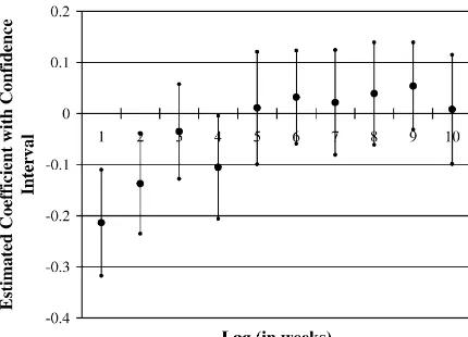
To this point, we have examined up to four lags. However, it is possible that dis-placement could operate over an even longer time horizon. To examine this possibil-ity, we calculate IV estimate for both violent and property crime in which we include up to ten lags and present the results in Figures 4a and 4b. Note that these results are directly comparable to the OLS estimates shown in Figures 2a and 2b. The top panel shows the results for violent crime. As we saw earlier, the first, second, and fourth lags are statistically significantly different from zero. The others hover around zero but are not consistently of one sign or another. At20.37, the sum of the ten lags is negative and statistically significant at the 10 percent level, suggesting that all of the displacement in violent crime occurs within a month. The bottom panel shows the results for property crime. In contrast to the results we found earlier, none of the lags is statistically different from zero. Furthermore, the sum of lags is only20.14 and statistically insignificant. Though the point estimates suggest that little displace-ment occurs over 10 weeks for property crime, the standard error on the sum of co-efficients is too large to rule out substantial displacement. For both violent and
Figure 4a
IV Estimates of the Relationship between Current and Lagged Violent Crime
property crime, however, the results do stand in stark contrast to the positive OLS estimates.
E. Estimates by Specific Crime Categories
It is of great interest to establish how our results vary by type of offense. This is com-plicated, however, by the fact that temporal displacement may occur across different types of crime. For example, an aggravated assault that is prevented by adverse weather conditions may result in a simple assault in a later period.27For this reason, a regression of simple assault on lagged simple assault may violate the assumptions necessary for valid instrumental variables identification. In particular, the instru-ments (lagged temperature and precipitation) may influence simple assault in the cur-rent period not only through its effect on lagged simple assault, but also through its effect on lagged aggravated assault or some other type of related crime in the prior period. To overcome this issue, when examining the effect of lagged crime on par-ticular types of crime, we estimate models in which the left-hand-side variable is the
Figure 4b
IV Estimates of the Relationship between Current and Lagged Property Crime
Notes: Panels show the IV estimates from a regression of current property crime on 10 lags. The unit of observation is a jurisdiction-week. All crime rates are computed by dividing the actual number of crimes during a week by the average number of weekly crimes within the jurisdiction. Other cova-riates include average temperature and total precipitation in the current period, jurisdiction-year fixed effects, jurisdiction-specific fourth order polynomials in day-of-year, and fixed effects for month. Lagged crime is instrumented using lagged average temperature and total precipitation. See the text for more details. Standard errors in parenthesis are clustered at the state*year*month level. Observa-tions are weighted by the mean number of all crimes within the jurisdiction.
rate of the specific type of crime under examination while the right-hand-side vari-able is a lagged measure of allviolent or property crime.28
Table 4 shows the findings for violent crime. The results suggest that an exogenous increase in violent crime leads to subsequent reductions in most violent crime cate-gories. In particular, a 10 percent increase in allviolent crime reduces simple and aggravated assaults by 3.5 and 2.9 percent respectively. Similarly, a 10 percent increase in all violent crime reduces violent crime against family members and indi-viduals known to the offender by nearly 3.0 percent over one week. We see similar effects for crimes with and without weapons. The IV estimate for violent crime by strangers is not statistically significant, though the point estimate suggests some dis-placement.29In all cases, when examining a four-lag model, we observe substantial displacement for all types of violent crime.30While our specification allows us to examine whether or not displacement occurs for particular crimes, it is not possible to compare the magnitudes of the coefficients across crime types. Still, these models allow us to conclude that temporal displacement of violence appears to operate for a variety of different types of violent crime.
In Table 5, we examine the findings for different types of property crime. Remem-ber that the simple labor supply framework outlined in Section II predicts that dis-placement should only operate for property crimes involving a fairly large monetary value, since the predicted income effect of stealing small items (for example, a candy bar) is likely trivial. Consistent with that prediction, the point estimates for the IV results suggest substantial displacement only for burglary and vehicle theft, although only the effects for vehicle theft are statistically significant. Interestingly, the 2SLS estimates for vehicle theft for four lags show enormous displacement. Because many property crimes—particularly those in the categories of larceny, shoplifting or robbery—involve relatively small amounts of money, it is not surprising that we find little effect for these crimes.
To more accurately capture property crime displacement, we estimate a model in which we measure property crime by thetotal valueof the property stolen during a particular period.31Interestingly, the results in Column 7 indicate statistically sig-nificant displacement over a one-week period. A 10 percent increase in the value of property stolen in one week is associated with a decline in value of property stolen in the following week by nearly 6 percent. The results for the four-lag model are not precise enough to be informative. Overall, these results for property crime suggest some displacement over a short time period, although the results are not as robust as for violent crime.
28. Note that these models assume that there is no displacement from violent to property crime, or vice versa. While this is probably not strictly true, it is likely that the magnitude of this type of displacement is second-order. Estimates from models where the right-hand-side is the specific crime under consideration are available upon request. In general, they are qualitatively similar to the ones shown here.
29. We expect gang violence might be disproportionately concentrated in the category of violent crime by strangers. To the extent that one expects the violent crime displacement to reflect gang activity, the insig-nificance of the displacement result for violence committed by strangers is a bit surprising. This could re-flect, however, the imprecision of the point estimates.
Dependent Variable: Crime in Periodt
OLS 0.083** 0.084** 0.064** 0.075** 0.080** 0.090** 0.036** 0.094** 0.021 (0.010) (0.012) (0.018) (0.016) (0.011) (0.015) (0.017) (0.010) (0.050)
— — — — — — — — —
IV 0.260** 0.354** 0.286** 0.265** 0.280** 0.120 0.268** 0.272** 0.185 (0.054) (0.063) (0.118) (0.091) (0.063) (0.104) (0.107) (0.066) (0.362) Sum of four lags
OLS 0.186** 0.200** 0.140** 0.199** 0.180** 0.219** 0.112** 0.209** 0.111 (0.010) (0.022) (0.032) (0.030) (0.022) (0.029) (0.033) (0.021) (0.079)
— — — — — — — — —
IV 0.536** 0.649** 0.567** 0.381** 0.498** 0.545** 0.543** 0.506** -0.447 (0.128) (0.151) (0.224) (0.182) (0.140) (0.212) (0.244) (0.165) (0.600)
Periodtweather Yes Yes Yes Yes Yes Yes Yes Yes Yes
Jurisdiction*year effects Yes Yes Yes Yes Yes Yes Yes Yes Yes
Table 4 (continued)
Dependent Variable: Crime in Periodt
All Violent
Month effects Yes Yes Yes Yes Yes Yes Yes Yes Yes
Jurisdiction-specific fourth order polynomial in day of year
Yes Yes Yes Yes Yes Yes Yes Yes Yes
Notes: Specifications in which the lagged crime rate is specific to the type of violent crime committed are inappropriate given that displacement of one type of violent crime might be manifested subsequently by a violent crime of a different type. Thus for all specifications, the lagged variable is the rate of all violent crimes. The de-pendent variable is number of crimes divided by the average number of those types of crimes in the jurisdiction. For the one-lag models, the parentheses contain standard errors that errors are clustered at the state*year*month level to take into account the correlation across jurisdictions within a state and within a jurisdiction over time. For the four-lag models, the parentheses contain the standard error of the sum of the coefficients on all four lags. Observations are weighted by the mean number of all crimes within the jurisdiction. * statistically significant at the 10 percent level; ** statistically significant at the 5 percent level.
The
Journal
of
Human
Dependent Variable: Crime in Periodt
Dependent Variable
All
Property Larceny Shoplifting Burglary
Vehicle
Theft Robbery
The total value of all stolen property
in periodt
(1) (2) (3) (4) (5) (6) (7)
One lag
OLS 0.279** 0.284** 0.176** 0.316** 0.257** 0.290** 0.170** (0.012) (0.012) (0.022) (0.028) (0.022) (0.035) (0.030) IV 20.201** 20.064 0.179 20.209 20.599** 20.009 20.582**
(0.083) (0.093) (0.192) (0.160) (0.213) (0.367) (0.265) Sum of four lags
OLS 0.429** 0.438** 0.336** 0.519** 0.416** 0.372** 0.343** (0.016) (0.018) (0.035) (0.042) (0.035) (0.052) (0.06) IV 20.326* 20.168 20.207 20.064 21.091** 20.007 23.99
(0.204) (0.201) (0.352) (0.313) (0.481) (0.642) (3.311)
Periodtweather Yes Yes Yes Yes Yes Yes Yes
Jurisdiction*year effects Yes Yes Yes Yes Yes Yes Yes
(Continued)
Jacob,
Lefgren,
and
Moretti
Table 5 (continued)
Dependent Variable: Crime in Periodt
Dependent Variable
All
Property Larceny Shoplifting Burglary
Vehicle
Theft Robbery
The total value of all stolen property
in periodt
(1) (2) (3) (4) (5) (6) (7)
Month effects Yes Yes Yes Yes Yes Yes Yes
Jurisdiction-specific fourth order polynomial in day of year
Yes Yes Yes Yes Yes Yes Yes
Notes: Specifications in which the lagged crime rate is specific to the type of property crime committed are inappropriate given that displacement of one type of property crime might be manifested subsequently by a property crime of a different type. Thus, for all specifications, the lagged variable is the rate of all property crimes. The dependent variable is number of crimes divided by the average number of those types of crimes in the jurisdiction. For the one-lag models, the parentheses contain stan-dard errors that errors are clustered at the state*year*month level to take into account the correlation across jurisdictions within a state and within a jurisdiction over time. For the four-lag models, the parentheses contain the standard error of the sum of the coefficients on all four lags. Observations are weighted by the mean number of all crimes within the jurisdiction. * statistically significant at the 10 percent level; ** statistically significant at the 5 percent level.
The
Journal
of
Human
VI. Robustness Checks
A. Temporal Displacement of Noncriminal Economic Activity
The main identifying assumption in our empirical strategy is that lagged weather conditions only influence current period crime through their influence on lagged crime. While high frequency variation in weather is unlikely to be correlated with many of the unobserved factors that determine the persistence of crime over time (for example, income levels, crime-prevention policies, etc.), weather may affect the intensity of noncriminal activity which, in turn, could influence the cost and/or benefit of crime. If inclement weather causes people to stay home in one period, for example, it may result in greater than expected economic activity in the following period, which could increase the benefits of crime (by increasing the availability of victims, for example). More generally, if weather displaces noncriminal activity and this activity influences the cost/benefit of criminal activity, our estimates may be biased. To assess the empirical importance of this concern, we first provide evidence re-garding the extent to which noncriminal activity is displaced by weather conditions. Though few measures of economic activity are reported at a sufficiently high fre-quency to examine this issue, we have collected information from the Federal High-way Administration (FHWA) that includes daily measures of traffic from in-road monitors in over 20,000 locations throughout the United States for 2000–2001. We regard traffic as a good summary measure for noncriminal economic activity.32 We aggregate this data to the county-week level, so that our primary outcome mea-sure is the number of vehicles counted in a particular county during a given week.33 Using data on weekly vehicle traffic for states represented in our sample, we find that weather conditions have only a small correlation with vehicle traffic. This is ex-tremely informative itself because if weather does not have a strong impact on this type of economic activity over a one-week period, it is unlikely that weather would induce substantial amounts of displacement to bias our estimates. Table 7 shows that when we instrument lagged traffic with lagged weather conditions, we find no evi-dence of temporal displacement over one or four weeks, though the standard errors are in some cases quite large.34This is also inconsistent with widespread temporal displacement of economic activity.
32. The traffic volume data includes hourly traffic counts for each traffic station provided by permanent in-road traffic monitors. Geographic identifiers allow one to link each station to states and counties. Traffic data are available for 66 of the 92 counties included in the crime analysis. Recall that our primary analysis sample for crime includes 116 jurisdictions in 92 counties in 17 states. For more information on the traffic data, see: Office of Highway Policy Information at http://www.fhwa.dot.gov/policy/ohpi.
33. To be consistent with the crime estimates, we normalize these measures by dividing weekly counts by the average for that county over the sample period.
Table 6
Jurisdictions Included in the Analysis
Jurisdiction Years in Sample Jurisdiction Years in Sample Jurisdiction Years in Sample
Adams County, CO 1997–2001 Grand Forks, ND 1995–2001 Paducah, KY 1998–2001 Aiken County, SC 1995–2001 Greenville Cnty, SC 1995–2001 Petersburg, VA 1995–2001 Akron, OH 1998–2001 Greenville, SC 1995–2001 Pocatello, ID 1995–2001 Albemarle County, VA 1997–2001 Greenwood, SC 1995–2001 Pontiac, MI 1997–2001 Alexandria, VA 2000–2001 Hamilton Cnty, OH 2000–2001 Portsmouth, VA 2000–2001 Anderson County, SC 1995–2001 Hampton, VA 2000–2001 Provo, UT 1995–2001 Arapahoe County, CO 1997–2001 Henrico County, VA 1999–2001 Redford, MI 1997–2001 Aurora, CO 1997–2001 Horry, SC 1995–2001 Richland County, SC 1995–2001 Austin, TX 1998–2001 Huntington, WV 2000–2001 Richmond, VA 2000–2001 Battle Creek, MI 1995–2001 Hutchinson, KS 2000–2001 Riley Cnty, KS 2000–2001 Beaufort County, SC 1995–2001 Idaho Falls, ID 1995–2001 Roanoke, VA 1999–2001 Berkeley County, SC 1995–2001 Iowa City, IA 1995–2001 Rock Hill, SC 1995–2001 Boise, ID 1995–2001 Jackson, TN 1999–2001 Roseville, MI 1996–2001 Burlington, VT 1999–2001 Jefferson County, CO 1997–2001 Saginaw, MI 2000–2001 Cedar Rapids, IA 1999–2001 Johnson City, TN 1998–2001 Salina, KS 2000–2001 Charleston County, SC 1995–2001 Junction City, KS 2000–2001 San Angelo, TX 2000–2001 Charleston, SC 1995–2001 Kalamazoo, MI 2000–2001 Sandy, UT 1995–2001 Charleston, WV 1999–2001 Kingsport, TN 1998–2001 Sioux City, IA 1995–2001
The
Journal
of
Human
Cherokee County, SC 1995–2001 Lakewood, CO 1997–2001 Spartanburg, SC 1995–2001 Chesterfield Cnty, VA 1999–2001 Layton, UT 1995–2001 Spotsylvania Cnt, VA 1999–2001 Cincinnati, OH 1998–2001 Lexington Cnty, SC 1995–2001 Springfield, MA 1996–2001 Clarksville, TN 1998–2001 Loudoun County, VA 1999–2001 Stafford County, VA 1997–2001 Cleveland, TN 1999–2001 Lynchburg, VA 2000–2001 Suffolk, VA 1997–2001 Coeur D’Alene, ID 1995–2001 Memphis, TN 2000–2001 Sumter, SC 1995–2001 Colorado Springs, CO 1997–2001 Murfreesboro, TN 1998–2001 Twin Falls, ID 1995–2001 Columbia, SC 1995–2001 Murray, UT 1997–2001 Virginia Beach, VA 1999–2001 Columbia, TN 1998–2001 Muskegon, MI 2000–2001 Warren, MI 1999–2001 Conroe, TX 1998–2001 Myrtle Beach, SC 1995–2001 Waterford, MI 2000–2001 Council Bluffs, IA 1995–2001 Nampa, ID 1995–2001 Waterloo, IA 1995–2001 Danville, VA 2000–2001 Nashville, TN 2000–2001 West Jordan, UT 1995–2001 Davenport, IA 1995–2001 Newark, OH 1998–2001 West Valley, UT 1996–2001 Dayton, OH 1998–2001 Newport News, VA 1998–2001 Worcester, MA 1995–2001 Des Moines, IA 1995–2001 Norfolk, VA 1999–2001 Wyoming, MI 1999–2001 Fairfax County, VA 2000–2001 North Charleston, SC 1995–2001 York County, SC 1995–2001 Fargo, ND 1995–2001 Norwalk, CT 1999–2001
Florence County, SC 1995–2001 Oakland County, MI 1997–2001 Florence, SC 1995–2001 Olathe, KS 2000–2001 Garden City, KS 2000–2001 Orangeburg Cnty, SC 1995–2001
Jacob,
Lefgren,
and
Moretti
Table 7
OLS and IV Estimates of the Relationship between Current and Lagged Traffic
Dependent Variable: Traffic Volume in Periodt
OLS IV OLS IV OLS IV OLS IV
(1) (2) (3) (4) (5) (6) (7) (8)
Traffict-1 0.633** 0.040 0.618** 0.163 0.811** 20.094 0.753** 0.092 (0.024) (0.219) (0.030) (0.214) (0.009) (0.172) (0.016) (0.207) Traffict-2 — — 20.091** 20.045 — — 20.029* 20.068
(0.029) (0.207) (0.016) (0.220)
Traffict-3 — — 0.025 20.001 — — 0.041** 20.204
(0.031) (0.163) (0.017) (0.199)
Traffict-4 — — 0.031 20.120 — — 0.070** 20.254
(0.026) (0.220) (0.014) (0.322)
Sum of coefficients 0.633** 0.040 0.583** -0.002 0.811** -0.094 0.833** 20.435 (0.024) (0.219) (0.034) (0.450) (0.009) (0.172) (0.010) (0.789)
F-statistic from first-stage regression [p-value]
— 9.35 — — — 18.65 — —
[0.00] [0.00]
Observations 4,959 4,959 4,272 4,272 42,893 42,893 37,076 37,076
Notes: Standard errors in parenthesis. Standard errors are clustered at the state*year*month level to take into account the correlation across jurisdictions within a state and within a jurisdiction over time. In Columns 1 to 4, controls include periodtweather controls, jurisdiction*year fixed effects, month fixed effects, and jurisdiction-specific fourth order polynomial in week of year. In Columns 5 to 8 controls include periodtweather controls, jurisdiction fixed effects, year fixed effects, month fixed effects and state-specific fourth order polynomial in day-of-year. The sample in Columns 1 to 4 includes all 66 of the 92 counties in the crime sample for which traffic data are available. The sample in Columns 5 to 8 includes all 570 counties in the 17 states included in the crime analysis that also have traffic data. * significant at the 10 percent level; ** significant at the 5 percent level.
The
Journal
of
Human
As a second piece of suggestive evidence on temporal displacement in economic activity, we estimate separate models for indoor and outdoor crime. If weather indu-ces displacement in noncriminal activity, we would expect to see more (less) outdoor activity after a bad (good) spell of weather. If crime follows economic activity, we also should expect more outdoor crime following bad weather (and vice versa) but
less indoor crime. This suggests that our displacement results would be focused on outdoor as opposed to indoor crime. For violent crime, we find that an exogenous increase in violent crime leads to statistically significant reductions in both outdoor and indoor violence over a four-week period, although the one-week effect is only statistically significant for indoor crime. The property crime estimates are uniformly negative and similar in magnitude for indoor and outdoor crime, but only signifi-cantly different from zero in one of four cases (see Table 10 in Jacob, Lefgren, and Moretti 2004).
A third suggestive piece of evidence regarding the potential bias from the dis-placement of economic activity can be obtained by examining the relationship be-tween offenders and victims for violent crime. It seems plausible that interactions with family members would be least sensitive to the degree of noncriminal economic activity. In Table 7, we showed that an exogenous increase in violent crime leads to statistically significant reductions in the amount of violence against family members during the following week. Although by no means definitive, taken together these results suggest that our finding of temporal displacement is not driven by displace-ment of noncriminal economic activity.
B. Endogenous Police Staffing Levels
A second concern is that police may departments may change staffing levels in re-sponse to weather conditions or small fluctuations in the crime rate. For example, police may know that on hot days there is more crime and thus increase the number of working officers on those days. Such behavior amplifies or attenuates the correla-tion between weather and crime but ultimately acts simply as another cost factor. Thus the consistency of our IV estimates is unaffected by such behavior.
A more serious concern would be if current staffing levels were correlated to lagged weather conditions. This would violate the exclusion restriction necessary for satisfactory identification. Such a situation might exist if police departments ad-justed staffing levels going forward in response to small fluctuations in crime rates associated with weather conditions. To reduce concerns on this front, we contacted several police departments in our sample. The responding agencies indicated that they did not adjust staffing levels in response to nonemergency weather conditions. Furthermore, changes in staffing levels were proactive—not reactive. In other words, departments might increase staffing levels in response to a parade butnotin response to a temporary and unexpected increase in number of reported offenses. These responses suggest that the endogeneity of police staffing levels is unlikely to be a meaningful source of bias.
C. Persistence in Weather