INFORMATION FILTERING WITH SUBMAPS FOR
INERTIAL AIDED VISUAL ODOMETRY
M. Kleinerta,∗
U. Stillab
a
Department Scene Analysis, Fraunhofer IOSB, Gutleuthausstr. 1, 76275 Ettlingen, Germany - [email protected]
b Photogrammetry and Remote Sensing, Technische Universit¨at M¨unchen, Arcisstr. 21, 80333 M¨unchen, Germany - [email protected]
KEY WORDS:Indoor Positioning, Inertial Aided Visual Odometry, Bundle Adjustment, Submapping
ABSTRACT:
This work is concerned with the fusion of inertial measurements (accelerations and angular velocities) with imagery data (feature points extracted in a video stream) in a recursive bundle adjustment framework for indoor position and attitude estimation. Recursive processing is achieved by a combination of local submaps and the Schur complement. The Schur complement is used to reduce the problem size at regular intervals while retaining the information provided by past measurements. Local submaps provide a way to propagate the gauge constraints and thereby to alleviate the detrimental effects of linearization errors in the prior. Though the presented technique is not real-time capable in its current implementation, it can be employed to process arbitrarily long trajectories.
The presented system is evaluated by comparing the estimated trajectory of the system with a reference trajectory of a prism attached to the system, which was recorded by a total station.
1. INTRODUCTION
1.1 Importance for autonomous indoor localization
For first responders or special forces operating in unknown en-vironments, positioning is a crucial capability. Besides position, users are often interested in their heading, i.e. the direction they are facing. Both can in principle be computed from global navi-gation satellite system (GNSS) signals, but recovering the head-ing requires that the user is movhead-ing.
However, in indoor scenarios or urban canyons, where GNSS sig-nals cannot be received or are severely distorted due to multipath effects, alternative methods to determine position are required. In contrast to position, heading can be obtained by magnetome-ter measurements almost everywhere, but the local magnetic field may be disturbed by reinforced concrete inside or near building walls.
Thus, indoor positioning systems for firefighters have been de-veloped using radio beacons which have to be placed around the site of operation before a mission starts (McCroskey et al., 2010). Such systems typically combine position estimates ob-tained by trilateration with relative motion estimates. In the con-text of pedestrian navigation, such relative motion measurements are often obtained by inertial sensors placed on the foot where the foot’s stand still phase can be exploited to obtain accurate motion estimates even with inertial sensors of relatively low quality. But in this case the question how estimates of the foot’s motion can be fused with measurements of devices attached to the torso needs to be addressed.
One possibility that does not rely on external infrastructure is to fuse measurements from a camera and an inertial measurement unit (IMU), to estimate one’s position as well as attitude rela-tive to a starting point. The combination of visual and inertial measurements is attractive because of the complementary error characteristics of these sensors. Compared to systems relying on foot-mounted inertial sensors, this setup allows to put all sensors in a single housing fixed to the torso of a person and it does not rely on a special motion pattern.
∗Corresponding author.
1.2 Related Work
Motivated by the observation that the detrimental effect of lin-earization discovered by (Dong-Si and Mourikis, 2011) is closely related to the problem of gauge fixing in estimation problems, the approach presented in this work tackles this problem by applying the local submapping procedure presented in (Pini´es and Tard´os, 2008) in the context of information filtering. Local submaps pro-vide a way for consistent gauge definition and thus may propro-vide a way to control the observable subspace. However, a formal proof of this statement has to be deferred to future work.
1.2.1 The main contribution of this paper is presented in Sec. 2.6, where it is shown how a new local reference coordinate system is set up before marginalizing old states.
2. INFORMATION FILTERING WITH SUBMAPS
2.1 Coordinate systems and notation
Several coordinate systems are used in the following presentation of the system model. All coordinate systems are assumed to be right-handed. The purpose of the algorithm presented here is to estimate the system’s trajectory and a sparse map of point feature locations relative to an established frame of reference, which is henceforth called navigation frame{n}. Its z-axis points in the direction of local gravity, but its origin and rotation about the z-axis may be chosen arbitrarily, reflecting the freedom in selecting the gauge constraints. If some guess of initial position and head-ing is available, the free parameters can be adjusted accordhead-ingly. Each local submap is build up relative to its own frame of ref-erence{si}, whereirefers to the number of the local map. The
submap index is omitted wherever confusion is not possible. Fur-thermore, the sensor system’s frame of reference (body frame) is denoted{b}. It is assumed that the rigid transformations between all sensors are fixed and known, possibly from a calibration pro-cedure. As a result, all sensor readings can be written w.r.t. the body frame.
The rigid body transformation between two frames,{a}and{b}, is described by a pair consisting of a rotation matrix (direction cosine matrix)Ca
b and a translation vector a
For the refinement of initial estimates, the error state notation is used (Farrell and Barth, 1999). Estimates are marked by a hat(ˆ·), measurements by a bar(¯·), and errors by a tilde(˜·). For most state variables an additive error model can be applied:(˜·) = (·)−(ˆ·). However, attitude error is represented by a rotation vectorΨa
b,
which is an element of the Lie algebraso(3)belonging to the group of rotation matricesSO(3).
Attitude errors are corrected by left-multiplication:
Cba=C(Ψ a b) ˆC
a
b (1)
The relationship between a rotation vector and the corresponding rotation matrix is C(Ψ) = exp(Ψ) ≈ I +⌊Ψ⌋×. This can also be stated asΨ = vec(log(C(Ψ))). Rotation vectors can be mapped between frames just like ordinary vectors using the adjoint mapAdg. These facts and more background material can be found in (Murray et al., 1994). Whereas attitude is represented by rotation matrices here, it is represented by quaternions in the implementation.
To handle heterogeneous states, which may be composed of ro-tation matrices and vectors, the different entities are combined to a tuple. The tuple is then corrected by applying the corrections to its elements individually, i.e. using Eq. 1 for rotations and ad-dition for vectors. The operators ‘⊕’, ‘⊖’ are used to mark this operation on the tupel’s elements:t= ˆt⊕˜t. Note, that the error
˜tbelongs to a vector space.
2.2 Camera measurement model
A camera can be regarded as a bearings measuring device. Thus it is assumed that a camera projection modelπ(.) is available, which allows to calculate the projection of a 3D-point onto the image plane and its inverse. The projection of landmark number
jonto image planeiis given by:
¯
zij = πi(bXj) +
vij (2)
Wherevij is an error term, which is usually assumed to arise from a zero-mean white Gaussian noise process with covariance
Σcam.
2.3 IMU measurement model
IMUs measure angular velocityωand specific forcearelative to their own reference frame. This work adopts the common as-sumption that the measurement noise can be described by the combination of a slow-varying bias and additive zero mean white noise:
Here, baand bg contain accelerometer and gyroscope bias and
na,ngare the corresponding noise terms.
Integrating the inertial measurements yields an estimate of the sensor system’s motion during the integration interval. For this purpose the inertial mechanization equations are implemented w.r.t. the strapdown frame, as suggested by (Lupton, 2010). As a consequence, the error of the rigid body transformation relating the{n}to the{s}frame does not affect the projection of a land-mark onto the image plane, because the quantities in Eq. 2 only depend on the system’s position w.r.t. {s}. Additionally, intro-ducing an intermediate{s}-frame facilitates the enforcement of the conditional independence properties for the local submaps as detailed in Sec. 2.6. The inertial mechanization equations for one timestep can be stated as follows:
s
Where the quantities on the left hand side refer to the point in time
In the above equations,τ is the timespan between two samples andng = [0,0,9.81]T
is the vector of gravitational accelera-tion. Note, that at least the attitude (roll and pitch angles) of the {n}frame relative to the{s}frame needs to be known to com-pensate gravitational acceleration. By setting the noise terms to zero and replacing all quantities by their estimated counterparts, the mechanization equations for estimated quantities follow from Eqs. 5-10.
Combining the state variables into a tupel st and writing the above equations as a single state transition functionfgives:
st+τ = f(st,u,n) (11)
≈ f(ˆst,u,0)⊕(Φ˜st+Gn) (12)
˜
st+τ = st+τ⊖f(ˆst,u,0) (13)
= Φ˜st+Gn (14)
Here, u contains all inertial measurements, ncontains all the noise terms, andΦ,Garef’s derivatives w.r.t. sandn. When calculating the Jacobians, the states related to attitude require spe-cial attention. Explicitly writing Eqs. 5 and 8 in terms of incre-mental rotations yields:
Using the facts about rotation vectors and matrices presented in Sec. 2.1, the state transition function forΨs
b is obtained from
Likewise, Eq. 16 yields the derivatives ofsaw.r.t.Ψs b,Ψ
Thereby, the entries ofΦare obtained by standard calculus from Eqs. 5-10 and 18-20.
Concatenating the non-linear state transition functions (Eq. 11) yields the state transition functionf′
=fk+m:mfor several
mea-surements between measurement numbermandk+m. The Ja-cobiansΦ,Gprovide a linear error propagation model between successive inertial measurements. To propagate the error over several inertial measurements between exteroceptive sensor read-ings, a cumulative state transition matrixΦ′
and covarianceΣ′ a linearized constraint for successive pose and velocity estimates between exteroceptive sensor readings, which can be used within a bundle adjustment framework.
2.4 Inference
Graphical models have become popular tools to formalize op-timization problems. There are two types of graphical models which are commonly used: Dynamic Bayesian networks (DBNs) and factor graphs (Bishop, 2006). While DBNs are useful to ex-amine the stochastic independence properties between variables in a model, factor graphs relate directly to the Gauss-Newton algorithm in the case that the distribution of state variables is jointly Gaussian. Thus, factor graphs can facilitate the imple-mentation and description of optimization problems by providing a formal framework, which directly translates to a class hierar-chy in object-oriented programming languages. In what follows, a factor graph formulation is used in the presentation of the esti-mation procedure, especially the marginalization of older states.
A factor graph consists of vertices, which represent state vari-ables, and edges representing relationships or constraints between them. Typically there are different kinds of edges connecting dif-ferent kinds of state variables. The relationship between vertices associated with an edge is expressed by an objective function that often depends on measured values. The strength of a constraint is determined by a weight matrix, typically the inverse of a mea-surement covariance. The following types of constraint edges are of interest in this work:
Landmark measurement: Each landmark observation gives rise to a constraint according to the model described in Sec. 2.2. The constraint function is
hcam(Vlm,ij) = ¯zij−πi(bXj) (23)
with weight matrixΛcam = Σ−1
cam. Vlm,ij is the set of
connected vertices. The number of vertices inVlm,ij
de-pends on the employed parameterization and measurement model. For instance,Vlm,ijmay contain a vertex containing
the camera’s calibration or a landmark anchor vertex.
Motion constraint: Motion constraints can be obtained by inte-grating inertial measurements as described in Sec. 2.3. The constraint can be stated as:
himu(Vmotion,k+m:m) = Π (ˆsk+m⊖f(ˆsm,u,0)) (24)
The associated weight matrix isΛimu = Σ′−1
imu. In Eq. 24, Πprojects the error to the states corresponding to the sen-sor’s pose and velocity. The dimension of the error vec-tor is therefore nine. Hence, bias and global pose are not part of the projected error vector, but the projected constraint error depends on these states nonetheless. The vertices connected by a motion edge are: Vmotion,i:j =
{vTs
bi, vvi, vTbjs, vvj, vTsn, vbba,g}, where the trailing
Equality Constraint: Equality constraints between vertices are used to model slow varying random walk processes, like bi-ases:
heq({va, vb}) =a⊖b (25)
The corresponding weight matrix depends on the random walk parameters.
Transformation constraint: These are used when a new submap is created to link transformed coordinates of state variables to their estimates in the preceding submap. De-pending on the type of transformed vertices, there may be different types of transformation constraints. For velocity vertices the following constraint is used:
htrans,vel(
vav, vbv, vTa
b ) =
a v−Ca
b b
v (26)
The weight matrix is a design parameter that can also be used to model process noise.
Here, inference refers to the process of estimating the state of a system based on available measurements. The sets of all con-straint edges and all vertices belonging to the graph are denoted byEandV, respectively. Each edgee ∈ E connects a set of vertices denotedV(e). At the beginning of an inference step the current state dimension is calculated and each vertex is assigned an index in the state vectorx, which is formed by concatenat-ing the state of all relevant vertices. Then, an empty information matrixΩand information vectorξare created. LetHe be the
Jacobian of Edgee, w.r.t. its vertices. A normal equations system is built up based on the constraints defined by all edges:
Ω ← Ω +X
e∈E
HT
eΛeHe (27)
ξ ← ξ+X
e∈E
HT
eΛeǫe (28)
In Eq. 28, ǫe is the error associated with an edge and Λe its weight as described above. Some vertices can be fixed, for in-stance to enforce gauge constraints. In this case the correspond-ing rows and columns are deleted fromΩandξ.
Solving the normal equations yields a vector of improvements
˜
x+, which are applied to correct the current state estimate:
ˆ
xi+1= ˆxi⊕x˜+ (29)
In the implementation, the inference step is performed using the Levenberg-Marquardt algorithm based on the description in (Lourakis and Argyros, 2005).
2.5 Landmark parameterization
This work makes use of the feature bundle parameterization for landmarks (Pietzsch, 2008) in combination with the negative log parameterization (Parsley and Julier, 2008) for landmark depth. For this purpose all landmarks are assigned to an anchor pose, which is usually the pose of the sensor frame they were observed in first. Anchors are created by cloning the pose vertex of the associated sensor pose and adding an equality constraint edge be-tween the anchor and the associated sensor pose. Thus, they can be altered even when their associated pose has been marginal-ized. Only the anchor’s pose and the negative logarithm of the
depth of its associated landmarks are treated as free parameters during estimation. This reflects the point of view that the first observation of a feature determines its direction and all follow-ing observations are noisy measurements of the directions to the same point.
2.6 Marginalization of old states
To reduce problem size and thus processing time, this work com-bines conditionally independent local maps (Pini´es and Tard´os, 2008) and marginalization via the Schur complement (Dong-Si and Mourikis, 2011). Pose and velocity vertices are added to the graph for each detected keyframe until a maximum number of pose vertices is reached. In this case a new submap is cre-ated. The lastn/2pose and velocity vertices remain in the graph, wherenis the number of sensor pose vertices present in the graph when marginalization is started. This enables further refinement of the associated estimates when new measurements are added. Additionally, all landmark vertices connected to the remaining poses via measurement edges, the bias vertex, and the global pose vertex remain in the graph. The set of remaining vertices is henceforth denotedVremand the set of vertices to
marginal-ize, which belong to the last submap, isVmarg. The set of edges
connecting at least one vertex in Vmarg is denotedEconn and
Vconnare all vertices connected by at least one Edge inEconn.
Vborder is the set of remaining vertices which are connected to
vertices inVmargvia an edge inEconn.
The vertices remaining in the graph are transformed to a new co-ordinate system whose origin is the first pose vertex present in the new submap. To this end, the vertices inVborderare cloned. The
resulting set of new vertices is thenVnew. A coordinate
transfor-mation is then applied to each vertex in this set to transform it to the origin of the new map and a new edge is created and added toEnew, the set of new edges. This edge generally connects the
new vertex, its template inVborder, and the pose vertex that
de-termines the transformation and becomes the first pose vertex in the new map. Note however, that different types of vertices in
Vborder are affected by this coordinate transformation in
differ-ent ways and are thus connected to their counterparts inVnewby
different kinds of edges. E.g., the bias vertices are not affected at all by a change of coordinates. Hence, the bias vertices for the new submap are connected to the preceding bias vertices via an equality constraint whose uncertainty is determined by the bias random walk parameters. Furthermore, since the new first pose vertex is the new map’s origin, its coordinates in the new map are fixed and it is not connected to any vertex inVborder at all. For
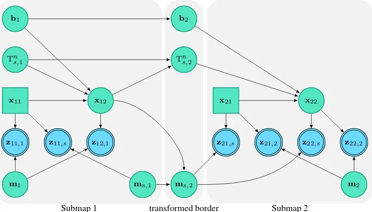
those remaining vertices which are not connected to the previous submap, it is sufficient to transform the coordinates to the new origin. New edges do not have to be inserted in this case. Fig-ure 1 illustrates the structFig-ure of the network after performing the coordinate transformation and adding new vertices as a DBN. It can be seen that the new layer of transformed border vertices ren-ders the remaining vertices conditionally independent from the vertices in the previous submap. Hence, it constitutes a sufficient statistic for the remaining vertices.
Next, a set of transformed vertices (Vtrans) is defined containing
Submap 1 transformed border Submap 2
b1 b2
Tn
s,1 Tns,2
x11 x12 x21 x22
z11,1 z11,s z12,1 z21,s z21,2 z22,s z22,2
m1 ms,1 ms,2 m2
Figure 1. Dependencies between nodes in the Bayesian network corresponding to the SLAM problem before performing marginal-ization with the Schur complement. Green nodes with a single boundary are state variables. Rectangular green nodes represent states which are held fixed during optimization to impose the gauge constraints. Blue nodes with a double boundary represent measurements (landmark observations). Inertial measurements and velocities are not shown in this simplified network.
Vmarg=V \Vrem (30)
Econn={e∈E|∃vi∈Vmarg:vi∈V(e)} (31)
Vconn={v∈V|∃ei∈Econn:v∈V(ei)} (32)
Vborder=Vrem∩Vconn (33)
Vnew= cloneAndTransform(Vborder) (34)
Enew= createTransformationEdges(Vborder, Vnew) (35)
∀v∈Vrem\Vborder: applyTransform(v) (36)
Vtrans=Vnew∪(Vrem\Vborder) (37)
V′
=V ∪Vnew (38)
E′
=E∪Enew (39)
V′
marg=V
′
\Vtrans (40)
E′
conn={e∈E
′ |∃vi∈V
′
marg:vi∈V(e)} (41)
V′
conn={v∈V
′
|∃ei∈E
′
conn:v∈V(ei)} (42)
V′
rem=V
′
conn\V
′
marg (43)
Here, the function cloneAndTransform(V) clones each vertex in V and transforms its coordinates,
createTransformationEdges(V1, V2) creates constraint edges
between the vertices in V1 and V2, and applyTransform(v)
applies the coordinate transformation to vertexv. The applied coordinate transformation must not change the internal geometry of the network. Therefore, it is related to a S-transformation, which can be used to change between gauges during computa-tions (Triggs et al., 2000).
Letxdenote the state vector obtained by stacking the states of vertices inV′
remandy the state vector associated withV
′
marg.
First, a normal equations system is build up as described by Eqs. 27 and 28, but using only edges inE′
conn. Then the Schur
complement is used to marginalize the states iny, resulting in a new information matrix and -vector for the remaining statesx:
Ω′
x,x = Ωx,x−Ωx,yΩ −1
y,yΩy,x (44)
ξ′
x = ξx−Ωx,yΩ −1
y,yξx (45)
Next, a new edge,eprior, is created to hold the prior information
which is represented byΩ′
x,x andξ ′
x. To this end, all vertices
belonging toxare cloned and the cloned vertices are added to
V(eprior). Furthermore, the weight matrix for eprior is set to Ω′
x,x. To calculate the error associated with this edge, the vertices inV(eprior)are stacked to a tuplexprior. Then the edge error is calculated by:
hprior=xprior⊖x (46)
The error is initially zero becausexand xprior are equal, but when the estimate ofxis adapted due to new measurements, de-viations from xprior are penalized according to the weights in
Ω′
x,x. Finally, the marginalized vertices and all edges connecting to them can be removed from the graph since the corresponding information is now represented by the prior edge:
E = (E′ \E′
conn)∪ {eprior} (47)
V = V′ \V′
marg (48)
3. EXPERIMENTAL RESULTS
3.1 Simulation experiments
3.1.1 Scenario Experiments with real data demonstrate the applicability of an approach under similar conditions. When eval-uating real datasets, the results are probably affected by synchro-nization errors, systematic feature matching errors, inaccuracies of the employed sensor model, and sensor-to-sensor calibration errors. Thus, it is difficult to draw conclusions about the perfor-mance of the employed sensor data fusion algorithm alone based on the evaluation of real datasets.
−2 0 2 4 6
−30 −20 −10 0
y (m)
x (m)
5 10 15 20 25 0.05
0.1 0.15 0.2 0.25
error pos. x (m)
time (s) 5 10 15 20 25 0.05
0.1 0.15 0.2 0.25 0.3
error pos. y (m)
time (s)
5 10 15 20 25
0.2 0.4 0.6 0.8 1 1.2
error pos. z (m)
time (s)
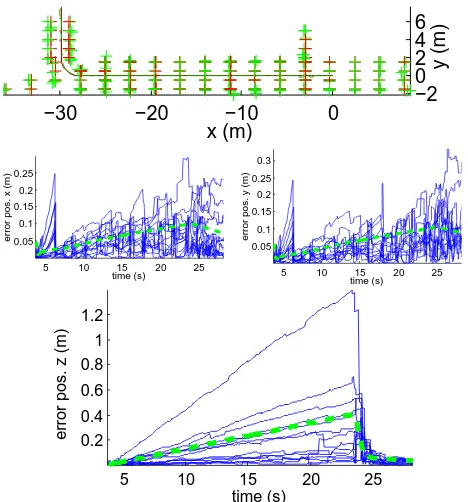
Figure 2. Evaluation of a simulated walk through a hallway. Top: Reference trajectory (dark red), estimated trajectory (dark green), landmark reference positions (red) and estimated landmark posi-tions (green) for one simulation run. Thereunder: Position error in the x-, y- and z-direction for 13 simulation runs (blue) with the square root of the Cram´er-Rao lower bound (dashed green).
performance of different approaches to structure and motion esti-mation from two views in (Weng et al., 1993) using the Cram´er-Rao lower bound (CRLB). The CRLB is a lower bound for the variance of unbiased estimators which can be stated as follows (Bar-Shalom et al., 2001):
Σ ≥ Ωˇ−1
(49)
WhereΩˇ is the Fisher information matrix, i.e., the information matrix built up in Eq. 27 with the JacobiansHecalculated at the
true values andΣis the covariance matrix for the estimation error. Eq. 49 is valid for Gaussian, zero-mean measurement noise.
Since the calculation of the CRLB requires knowledge of the true state values, its application is essentially limited to Monte Carlo simulations. In this case it is also possible to simulate zero-mean, normally distributed measurement noise, hence satisfying another prerequisite to the application of Eq. 49. It can not be assumed that the estimation process described in Sec. 2. is un-biased. However, as stated in (Weng et al., 1993) the CRLB can still be regarded as a lower bound for the mean squared error.
A walk through a hallway was simulated in order to compare the proposed method to the CRLB. The walk starts in the middle of a hallway that is approximately 3.5 m wide and 3 m high. Af-ter following the main hallway for approximately 30 m it turns to the right into a smaller corridor that is approximately 2.5 m wide. The trajectory of the sensor system’s origin was specified by aC2
-spline. The control points for this spline were chosen so as to resemble the typical up and down pattern of a walking person. White Gaussian noise was added to these control points to make the motion less regular. Another spline was used to de-termine the viewing direction for each point in time. The second derivative of the former spline can be calculated analytically and
was used to generate acceleration measurements. Likewise, gy-roscope measurements were generated by calculating the rotation vector pertaining to the incremental rotations between sampling points. The true acceleration and angular rate values obtained this way were distorted by artificial white Gaussian noise and constant offsets to match the sensor error model described in Sec. 2.3.
Image measurements were generated according to the model de-scribed in Sec. 2.2 using a fisheye projection model and the true values for landmark location and camera pose. To this end a backward-looking camera was assumed.
The CRLB was calculated once for each keyframe by building up the graphical model as described in Sec. 2.4 using all measure-ments available up to this point in time and setting the state vari-ables contained in each vertex to their true values. Then the Jaco-bians were calculated and the system matrix was built up accord-ing to Eq. 27. This matrix was inverted to obtain the CRLB for the point in time corresponding to the keyframe. Note that marginal-ization was not performed in the computation of the CRLB.
3.1.2 Results In order to illustrate the spread of estimation errors, the errors pertaining to position estimates in each direc-tion are shown in Figure 2 together with the square root of the calculated CRLB for 13 Monte Carlo runs using the scenario de-scribed in the previous section. The limitation to position errors in this investigation is justified by the fact that they depend on the remaining motion parameters through integration. Therefore, it can not be expected to achieve good position estimates when the estimates for attitude or velocity are severely distorted. When interpreting the error plots in Figure 2 it has to be considered that the optimization of the whole graph was only performed when the reprojection error exceeded a threshold at irregular time inter-vals. In the meantime the estimation error could grow arbitrarily. This explains the ragged appearance of the error curves.
For an estimator that attains the CRLB it can be expected that ap-proximately 70% of all error plots lie below the square root of the CRLB. This is because the CRLB is the lower bound on the error covariance and for a normally distributed variable approximately 70% of all realizations lie in the one sigma interval. Therefore, approximately four out of the 13 error plots shown in Figure 2 are expected to exceed the square root of the CRLB, if the estimator is efficient.
A visual inspection of the plots shows that the trend in the error curves generally follows the square root of the CRLB. Further-more, the number of error curves exceeding the square root of the CRLB is slightly higher than the expected number of four. This indicates that the proposed method does not make full use of the information available. However, the deviation from the CRLB appears to be acceptable in this example.
After approximately 24 sec., a drop in the position error plots and the square root of the CRLB can be observed. This corresponds to the point in time when the trajectory bends to the right into the next corridor, which goes along with a notable rotation about the yaw axis. A possible explanation for this behavior is that the roll-and pitch angles become separable from the acceleration biases by this motion. If the error in z-direction (height) is correlated with the roll- and pitch errors, this would also cause a correction of the estimated height.
3.2 Real-data experiments
-5 0 5 10 15 20 25 30 35 40 0 5 10 15 20 25 30 35 40
x (m)
y
(m)
0 10 20 30 40
0 5 10 15 20 25 30 35 40
x (m)
y
(m)
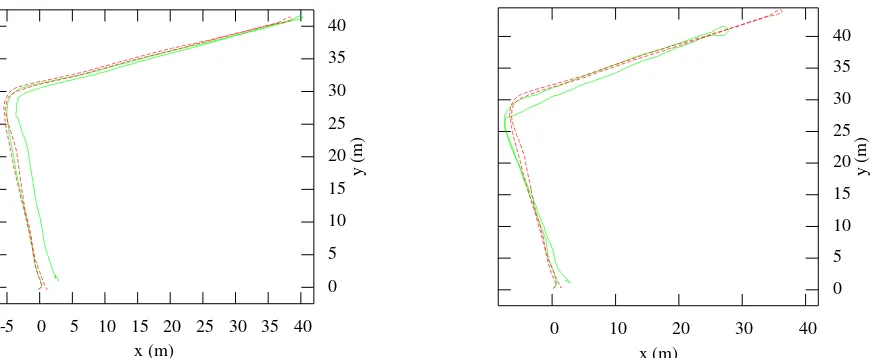
Figure 3. Experimental results for one run with the camera looking forward (left), and a run with the camera looking backwards (right). The reference trajectories recorded by the total station are shown as dashed red lines, the estimated trajectories are shown as green lines.
hallways and varying illumination conditions. In the experiments the sensor system was attached to the torso of a person walking through a hallway. For each test run, a reference trajectory was recorded by tracking the position of a prism with a total station while the system was recording data. The prism was attached to a rod which in turn was mounted on a plastic plate that was rigidly attached to the sensor system. The leverarm between the prism and the camera was calibrated prior to the experiments while be-ing in standstill. For this purpose, a mirror-based calibration pro-cedure similar to the one presented in (Hesch et al., 2009) was developed, which allows to obtain an estimate of the leverarm without the necessity to resort to additional sensors. Moreover, visual markers whose position were measured by the total sta-tion were placed such that they were in the camera’s field of view at startup. In combination with the leverarm, this allows to transfer the reference trajectory to the frame of reference the esti-mates are calculated in. The employed sensor system comprises an XSens MTi-G-700 IMU which triggered an industrial camera at approximately 28 Hz to obtain synchronized video data. The camera was equipped with a Fisheye-lens to facilitate the tracking of features in indoor scenarios.
To obtain a quantitative measure for the similarity of estimated trajectories to their associated reference trajectories, the trajecto-ries are downsampled to polygonal curves with an equal and fixed number of segments. Here, 250 segments were used. Then, the Fr´echet distance between the downsampled polygonal curves is computed using a publicly available implementation of the algo-rithm described in (Alt and Godau, 1995). The Fr´echet distance can be imagined as the minimum length of a rope needed to con-nect two curves while moving along them without going back-wards. Thus, it provides a parameterization-independent measure of the resemblance of polygonal curves. If the samples are evenly spaced we expect the error introduced by sampling to be below 0.5 m as long as the overall length of the trajectory is less then 125 m.
3.2.2 Results Figure 3 shows the results obtained for two walks under the conditions described in the previous section. Both experiments were conducted in the same hallway, but while the camera was pointing in walking direction during the first ex-periment (left figure), it was mounted on the pedestrian’s back during the second experiment (right figure). By visual inspection the estimated trajectory seems to match the reference trajectory well in the first experiment, but there is a significant error for
the second experiment. This is also reflected by the calculated Fr´echet distances of 2.3 m for the forward-looking and 8.4 m for the backward-looking configuration, respectively.
Due to the flexibility of the plastic plate, the rod holding the prism was able to swing. This resulted in a deviation of the prism’s position from the equilibrium position in the order of a few cen-timeters. However, it is assumed that this effect can be neglected compared to the estimation error, which is in the order of some meters.
The large deviation between the estimated and the reference tra-jectory observed for the run with the backward-looking camera shown on the right side in Figure 3 raises questions about the presence of systematic, unmodeled errors. The simulation results presented in Sec. 3.1.2 suggest that the backward-looking config-uration itself is not the cause of those errors.
At startup the walls with observed features were further away from the camera when it was looking backwards than in the first experiment with a forwad-looking camera. Hence, the prior for the depth of landmarks observed at startup described the true depth distribution better for the forward-looking configuration. However, an investigation of initial depth prior edges for the backward-looking configuration showed that their energy (i.e. the normalized sum of squared residuals) is generally small com-pared to the energy associated with measurement edges. Moover, prior edges for landmark depth with high energy are re-moved from the graph. Thus, prior edges should not contribute spurious information.
Figure 4. Observed drift of feature tracks over time. Left image: Red crosses mark detected features. Right image: Blue crosses mark the tracked features after 160 images (camera facing back-wards).
5 10 15 0
0.1 0.2 0.3 0.4 0.5
rel. frequency
edge energy 2 4 6 8 10 0
0.1 0.2 0.3 0.4 0.5
rel. frequency
edge energy
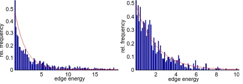
Figure 5. Relative frequency of landmark measurement edge en-ergy at one point in time for the real dataset with the camera fac-ing backwards (left) and for one simulation run (right). The cor-respondingχ2
pdf is drawn in red assuming a stdv. of 0.33 pixel for real measurement noise and 1 pixel stdv. for simulated mea-surement noise. Under the white Gaussian noise assumption the
χ2
pdf should provide a upper bound for the distribution of edge energies.
4. CONCLUSIONS AND FUTURE WORK
This work presents a local submapping approach to the inertial-aided visual odometry problem which allows to relinearize over past poses in an information filter framework. The key idea is to establish a consistent gauge based on local submaps. However, the quality of the trajectories estimated by the current approach does not seem to justify the excessive processing time due to repeated relinearization and inversion of densely populated nor-mal equations. A possible application of the presented algorithm would be to use it as a reference for simpler algorithms in situa-tions where accurate reference data is not available.
Future work should concentrate on improving the condition num-ber of the system matrix built up during the inference step. For this purpose it might be of interest to consider alternative gauge specifications. As a step towards real-time capability it would be beneficial to obtain a sparse approximation for the prior informa-tion matrix, for instance by applying a sparsificainforma-tion step as it is done in SEIFs (Thrun et al., 2005).
ACKNOWLEDGEMENTS
The authors would like to thank Mr. Zachary Danziger for pub-licly providing Matlab code to calculate the Fr´echet distance be-tween two polygonal curves.
REFERENCES
Alt, H. and Godau, M., 1995. Computing the fr´echet distance between two polygonal curves. International Journal of Compu-tational Geometry & Applications 5(01n02), pp. 75–91.
Bar-Shalom, Y., Li, X. R. and Kirubarajan, T., 2001. Estimation with Applications to Tracking and Navigation. John Wiley & Sons, Inc.
Beder, C. and Steffen, R., 2008. Incremetal estimation without specifying a-priori covariance matrices for the novel parameters. In: CVPR Workshop on Visual Localization for Mobile Platforms (VLMP).
Bishop, C. M., 2006. Pattern Recognition and Machine Learning. Springer Science+Business Media, LLC.
Dong-Si, T.-C. and Mourikis, A. I., 2011. Motion tracking with fixed-lag smoothing: Algorithm and consistency analysis. In: Robotics and Automation (ICRA), 2011 IEEE International Con-ference on, IEEE, pp. 5655–5662.
Farrell, J. and Barth, M., 1999. The Global Positioning System & Inertial Navigation. McGraw-Hill.
F¨orstner, W. and G¨ulch, E., 1987. A fast operator for detection and precise location of distinct points, corners and centres of cir-cular features. In: Proceedings of the ISPRS Conference on Fast Processing of Photogrammetric Data, pp. 281–305.
Hesch, J. A., Mourikis, A. I. and Roumeliotis, S. I., 2009. Mirror-based extrinsic camera calibration. In: Algorithmic Foundation of Robotics VIII, Springer, pp. 285–299.
Jones, E. S. and Soatto, S., 2011. Visual-inertial navigation, map-ping and localization: A scalable real-time causal approach. The International Journal of Robotics Research 30(4), pp. 407–430.
Lourakis, M. I. and Argyros, A. A., 2005. Is levenberg-marquardt the most efficient optimization algorithm for implementing bun-dle adjustment? In: International Conference on Computer Vi-sion, 2005, Vol. 2, IEEE, pp. 1526–1531.
Lupton, T., 2010. Inertial SLAM with Delayed Initialisation. PhD thesis, School of Aerospace, Mechanical and Mechatronic Engi-neering, The University of Sydney.
McCroskey, R., Samanant, P., Hawkinson, W., Huseth, S. and Hartman, R., 2010. Glanser - an emergency responder locator system for indoor and gps-denied applications. In: 23rd Interna-tional Technical Meeting of the Satellite Division of The Institute of Navigation, Portland, OR, September 21-24, 2010.
Murray, R. M., Li, Z. and Sastry, S. S., 1994. A Mathematical Introduction to Robotic Manipulation. CRC Press.
Parsley, M. P. and Julier, S. J., 2008. Avoiding negative depth in inverse depth bearing-only slam. In: IEEE/RSJ International Conference on Intelligent Robots and Systems.
Pietzsch, T., 2008. Efficient feature parameterisation for visual slam using inverse depth bundles. In: Proceedings of BMVC.
Pini´es, P. and Tard´os, J. D., 2008. Large scale slam building conditionally independent local maps: Application to monocular vision. IEEE Transactions on Robotics pp. 1–13.
Sibley, G., Matthies, L. and Sukhatme, G., 2010. Sliding win-dow filter with application to planetary landing. Journal of Field Robotics 27(5), pp. 587–608.
Thrun, S., Burgard, W. and Fox, D., 2005. Probabilistic Robotics. The MIT Press.
Triggs, B., McLauchlan, P., Hartley, R. and Fitzgibbon, A., 2000. Bundle adjustment - a modern synthesis. In: B. Triggs, A. Zis-serman and R. Szeliski (eds), Vision Algorithms: Theory and Practice, Lecture Notes in Computer Science, Vol. 1883, Springer Berlin / Heidelberg, pp. 153–177.