Open GIS Consortium
35 Main Street, Suite 5Wayland, MA 01778 Telephone: +1-508-655-5858
Facsimile: +1-508-655-2237
Editor:
Telephone: +1-703-830-6516 Facsimile: +1-703-830-7096
The OpenGIS™ Abstract Specification
Topic 4: Stored Functions and Interpolation
Version 4
Copyright © 1999, Open GIS Consortium, Inc.
NOTICE
The information contained in this document is subject to change without notice.
The material in this document details an Open GIS Consortium (OGC) specification in accordance with the license and notice set forth on this page. This document does not represent a commitment to implement any portion of this specification in any companies’ products.
While the information in this publication is beleived to be accurate, the Open GIS Consortium makes no warranty of any kind with regard to this material including but not limited to the implied warranties of merchantability and fitness for a particular purpose. The Open GIS Consortium shall not be liable for errors contained herein or for incidental or consequential damages in connection with the furnishing, performance or use of this material. The information contained in this document is subject to change without notice.
The Open GIS Consortium is and shall at all times be the sole entity that may authorize developers, suppliers and sellers of computer software to use certification marks, trademarks, or other special designations to indicate compliance with these materials.
This document contains information which is protected by copyright. All Rights Reserved. Except as otherwise provided herein, no part of this work may be reproduced or used in any form or by any means (graphic, electronic, or mechanical including photocopying, recording, taping, or information storage and retrieval systems) without the permission of the copyright owner. All copies of this document must include the copyright and other information contained on this page.
The OpenGIS™ Abstract Specification Page i
Revision History
Date
Description
The Page iii
Table of Contents
1. Introduction... 1
1.1. The Abstract Specification ...1
1.2. Introduction to Stored Functions and Interpolation...1
1.2.1. Background on Coverages ...1
1.2.2. Why Stored Functions are Important ...1
1.2.3. The Status of Stored Functions...1
1.3. References for Section 1...2
2. The Essential Model for Stored Functions and Interpolation... 3
2.1. Definition of a Function ...3
2.2. Applications ...3
2.2.1. Functions assign property values to property names ...3
2.2.2. Functions assign coordinates to locations...3
2.2.3. Functions assign values to points in a coverage ...4
2.2.4. Images as functions ...4
2.2.5. Maps as functions...4
2.3. Stored Functions...5
2.3.1. Exhaustive Listing ...5
2.3.2. Rational Function Approximation...5
2.3.3. Stored Functions for Linear Referencing...5
2.3.4. Interpolation and Extrapolation ...5
2.3.9. Interpolation in Linear Reference Systems ...7
2.4. Interfaces on Stored Functions ...7
2.4.1. Construct Stored Function ...7
2.4.2. Evaluate Stored Function ...7
2.4.3. Expose Stored Function ...7
2.5. References for Section 2...7
3. Abstract Model for Stored Functions and Interpolation... 8
3.1. References for Section 3...8
4. Future Work... 9
1.
Introduction
1.1.
The Abstract Specification
The purpose of the Abstract Specification is to create and document a conceptual model sufficient enough to allow for the creation of Implementation Specifications. The Abstract Specification consists of two models derived from the Syntropy object analysis and design methodology [1].
The first and simpler model is called the Essential Model and its purpose is to establish the conceptual linkage of the software or system design to the real world. The Essential Model is a description of how the world works (or should work).
The second model, the meat of the Abstract Specification, is the Abstract Model that defines the eventual software system in an implementation neutral manner. The Abstract Model is a description of how software should work. The Abstract Model represents a compromise between the paradigms of the intended target implementation environments.
The Abstract Specification is organized into separate topic volumes in order to manage the complexity of the subject matter and to assist parallel development of work items by different Working Groups of the OGC Technical Committee. The topics are, in reality, dependent upon one another each one begging to be written first. Each topic must be read in the context of the entire Abstract Specification.
The topic volumes are not all written at the same level of detail. Some are mature, and are the basis for Requests For Proposal (RFP). Others are immature, and require additional specification before RFPs can be issued. The level of maturity of a topic reflects the level of understanding and discussion occurring within the Technical Committee. Refer to the OGC Technical Committee Policies and Procedures [2] and Technology Development Process [3] documents for more information on the OGC OpenGIS™ standards development process.
Refer to Topic Volume 0: Abstract Specification Overview [4] for an introduction to all of the topic volumes comprising the Abstract Specification and for editorial guidance, rules and etiquette for authors (and readers) of OGC specifications.
1.2.
Introduction to Stored Functions and Interpolation
1.2.1.Background on Coverages
Geographic Information Systems do more than model geospatial information. They also build and present displays that are intended to reveal to human viewers relationships that are otherwise difficult to detect. Here we are thinking of displays that reveal urban invasion of song bird habitat, the salinity of the Chesapeake during a hurricane, and other complex combination of phenomena.
We may, therefore, think of a coverage as a kind of display, as a kind of window with Cartesian coordinates. The abstract mathematical space of Cartesian coordinates for the window is called the Coverage Extent.
Coverages, in general, require two stored functions. The first relates Earth coordinates to the window coordinates in the Coverage Extent. This function is called “G”, and it maps from the coordinates of a SRS to the Coverage Extent coordinates.
The second function assigns values to points in the Coverage Extent. The values may be thought of as colors, as this is a common value space. But the values could be temperatures, a scalar
representing fitness of habitat for song birds, the name of owner of the parcel containing the point, and so on. The second function is called “R”, and is called the Schema Mapping. It takes values in the Schema Range.
1.2.2.Why Stored Functions are Important
Both functions, G and R, need to be finitely represented so that they may be shared across an interface. A function that is finitely represented is called a stored function. A typical stored function is a finite set of (domain, range) pairs together with an interpolation algorithm.
The OpenGIS™ Abstract Specification Page 2
This Topic Volume, Stored Functions, provides essential and abstract models for technology that is used widely across the GIS landscape. Its first heavy use is expected to occur in support of Coverage specifications (see Topic 6, The Coverage Type).
A Request for Proposals for Simple Coverages is expected to be released in early 1998. Responses to that request are expected to include significant Stored Function functionality. This Topic Volume will be updated upon acceptance of implementation specifications to keep it a consistant technical foundation for Coverage technology.
1.3.
References for Section 1
[1] Cook, Steve, and John Daniels, Designing Objects Systems: Object-Oriented Modeling with Syntropy, Prentice Hall, New York, 1994, xx + 389 pp.
[2] Open GIS Consortium, 1997. OGC Technical Committee Policies and Procedures, Wayland, Massachusetts. Available via the WWW as <http://www.opengis.org/techno/development.htm>.
[3] Open GIS Consortium, 1997. The OGC Technical Committee Technology Development Process, Wayland, Massachusetts. Available via the WWW as
<http://www.opengis.org/techno/development.htm>.
2.
The Essential Model for Stored Functions and Interpolation
2.1.
Definition of a Function
A relation between two sets, A and B, is a collection, R, of ordered pairs (a, b), where a ∈ A, and b
∈ B.
A function, f, is a special kind of relation. If f is a function relation between two sets, D and R, the first is called the Domain, and the second is called the Range. Here is the formal definition:
A function, f, is a set of ordered pairs, (d, r), where d ∈ D and r ∈ R, satisfying the following two conditions:
1.If d ∈ D, then there is an r ∈ R such that (d, r) ∈ f. 2.(d, r) ∈ f and (d, s) ∈ f implies r = s.
3.If (d, r) is an element of f, then we say “f assigns to d the value r,” or “ → r.” The two conditions state that a function assigns to each element of D one and only one element of R.
2.2.
Applications
There are many applications of functions in the OGC Abstract Specification.
2.2.1.Functions assign property values to property names
The assignment of a PropertyValue to each PropertyName in a feature schema creates a function whose domain is the collection of PropertyNames in the schema, and whose range is the set of tuples of valid corresponding PropertyValues. To be more specific, suppose a feature has a schema consisting of (PropertyName1, ...PropertyNameN) and suppose that the set of valid values that PropertyNameJ may take is denoted ValueSetJ. Now a specific instance of a feature assigns to PropertyNameJ exactly one value from ValueSetJ, and this is true for each j from 1 to N. So, the instance of a feature caused N functions to be specified. These N functions could be wrapped into a single function where the vector (PropertyName1, ..., PropertyNameN) is related to a unique vector from the N-dimensional space (ValueSet1 ⊗ ValueSet2 ⊗ ... ⊗ ValueSetN).
Do not be confused by the fact that the ValueSets are often finite, and called Domain Lists. To be consistent, they should be called Range Lists, but the term Domain List seldom causes confusion.
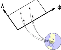
2.2.2.Functions assign coordinates to locations
A Spatial Reference System is a function. Its domain is the set of real world locations (or, to be more specific, the collection of “corners” of interest in our Project World.) The range is the collection of coordinate-tuples that make sense for the Spatial Reference System selected.
ϕϕ
λλ
Figure 2-1. A Spatial Reference System as a Function
For example, if the (Longitude, Latitude) (degrees) SRS is used, then the range is {(λ, ϕ): -180 < λ
The OpenGIS™ Abstract Specification Page 4
In the case of a Linear Reference System, the range is {(SegID, offset): where SegID is the Identification of any linear segment under consideration, and offset is a scalar that specifies a position on the linear segment.
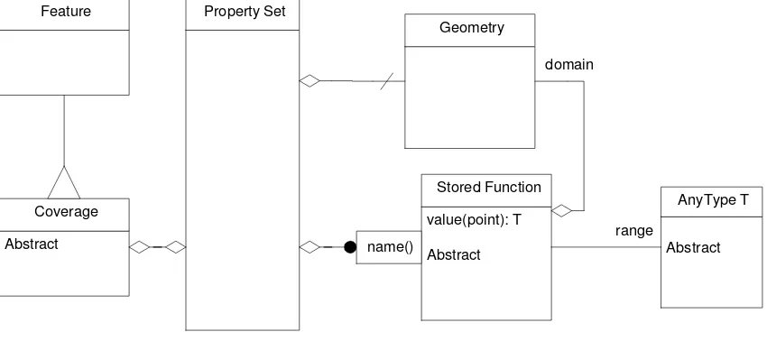
2.2.3.Functions assign values to points in a coverage
An important class of functions occur in coverages. A coverage is a subtype of feature. A coverage is associated with an abstract mathematical coordinate space called the Coverage Extent. A function called the Schema Mapping has the Coverage Extent (or a subset of it) as its domain. The range of the Schema Mapping is called (appropriately enough) the Schema Range. The Schema Mapping can be extremely complex, and may assign to different points in the Coverage Extent exotically different types of values in the Schema Range: scalars, colors, attribute values, and geometries.
In this sense, a coverage acts as a collection class for stored functions from points to instances of a value type. The relation between geometry and spatial reference system is the same as that in feature.
Figure 2-2. Functions in the Coverage Type
Notice that the range relation is to the class of type, and not to particular values.
2.2.4.Images as functions
A hard-copy photograph may be considered to be a function in several different ways. The brightness, b, of the photograph at a point (r, c) in photo coordinates is a function, b = B(r, c). Ordinary cameras form images using a pinhole or lens that accomplishes a perspectivity. This is a function relating lines of sight in 3-space (the field of view) to points on the 2-dimensional film. The photograph can be considered to be a perspectivity transform (a function) whose domain is the surfaces of objects in 3-space that first intersect the lines of sight. The function assigns to each point in this domain the point on the photograph where it is imaged.
Digital images are also functions in several additional ways. They may be thought of as samples (restricted domain) of ordinary photographs. Pixel values may be the result of a convolution of a continuous image with a sampling function. The reader is invited to investigate additional functions associated with digital images with a good text on the subject, such as [1].
2.2.5.Maps as functions
2.3.
Stored Functions
In mathematics, one often encounters functions that are defined using a rule that applies equally at every point in the domain. Examples are
z = f(x, y) = x2sin(y) (here the range is the set of real numbers ℜ, and the domain is ℜ⊗
ℜ)
z = [x] where [x] denotes the greatest integer smaller than x.
In other branches of science, such simple rules are seldom appropriate. There are several technologies for the computer storage (abstract representation) of complex functions. Some of them are listed below.
2.3.1.Exhaustive Listing
If a function has a finite domain, it may be feasible to list all the ordered pairs that define it. Digital images are frequently stored exhaustively. Soundings in bathymetric charts fall into this category, too.
2.3.2.Rational Function Approximation
If a function, f, takes real values (i.e., its range is ℜ) and is defined on a bounded subset of ℜ⊗ℜ, it may be possible to approximate f with a rational function. A rational function is a quotient of polynomials. The idea is to find a rational function, g, defined by
g(x, y) = P(x, y)/Q(x, y) (where P and Q are polynomials in x and y)
that is sufficiently close to f.
A polynomial in two variables has the form: P(x, y) = C00 + C01x + C10y + C02x
C02,... Cnm determine the polynomial P. Likewise, there is a list of coefficients that determine Q.
If P and Q can be determined so that the function g(x, y) = P(x, y)/Q(x, y) has the property
|f(x, y) - g(x, y)| < ε for all x, y
where ε is a tolerable margin of error, then f may be stored (and approximated) by storing the coefficients of the polynomials that define g, and using the values of g as sufficiently accurate approximations of the values of f.
Clearly, this idea can be extended to domains and ranges of arbitrary dimension.
2.3.3.Stored Functions for Linear Referencing
Suppose a curve, C, has starting point x0. There is a natural function, L, defined on the domain of
points on the curve and with range in the positive real numbers. It is: L(x) = distance along C from x0 to x. Since the curve, C, is defined by a finite geometry, L is easily stored.
2.3.4.Interpolation and Extrapolation
If a function is scalar valued and sufficiently continuous, it may be possible to store a finite number of its ordered pairs (x, y) (where x is an element of the domain, and y is an element of the range) and interpolate (or extrapolate) needed additional values with sufficient accuracy. Here is the general idea:
Suppose a function f needs to be stored. We assume f is scalar valued function on a bounded subset, B, of ℜ2. For integers i and j, with (i, j) ∈ B, store the information (i, j, f(i, j)). For (x, y)
where x and y are not both integers, the problem is to approximate f(x, y). One solution to the problem is bilinear interpolation from the four points with integer coordinates that surround the point (x, y). If this cannot be done with sufficient accuracy, one may store a denser (and larger) collection of precise values of f, and continue this process until the desired accuracy is achieved.
These ideas clearly extend easily to functions of arbitrarily many variables. For functions sampled on a grid in ℜ3, for example, this interpolation is call tri-linear.
The OpenGIS™ Abstract Specification Page 6
The bilinear interpolation scheme described above is often appropriate for recovering approximate function values using a gridded sample set. There are other scenarios in which different
interpolation and extrapolation schemes are more general.
2.3.5.1.Nearest Neighbor
The nearest neighbor method of recovering a function, f, assumes a finite collection of samples of f have been stored: {(xi, f(xi)): i = 1, ..., N}. To recover the value f(z) for an arbitrary point z, one
determines the closest point in {xi: i = 1, ..., N} to z. Say it is xj. The value f(xj) is used to
approximate f(z).
2.3.5.2.Constant Patches
A function can be set to a constant for a finite set of “patches.” The most common example of this is the polygon overlay that defines the function as a constant for each polygon in a collection of polygons. The usual methods for dynamic segmentation, raster images, and grid-cell based coverages also use this technique.
2.3.5.3.Triangulated Irregular Networks
Again, we assume that a finite collection of samples of f have been stored: {(xi, f(xi)): i = 1, ..., N}.
To recover the value f(z) for an arbitrary point z, one performs a triangulation on the points: {xi: i =
1, ..., N}. A triangulation on {xi: i = 1, ..., N} is a partition of the convex hull of the points into
triangles such that the set of vertices of the triangles is precisely {xi: i = 1, ..., N}. (This is often
done in a structured way called DeLauney Triangulation.) To recover the value f(z) for an arbitrary point z, one finds the triangle covering z, and interpolates the values stored at its three corners. Barycentric weighting is often employed in the interpolation.
2.3.5.4.Analytic Patches
More generally, a function can be stored using other analytical forms on a more general set of patches. Grid-post coverages use a variety of interpolation schemes, such as bilinear, biquadratic or bicubic polynomials. Spline functions define continuous functions (usually polynomial or rational functions) over patches in a similar manner. Most spline functions use quadrilateral patches in the coordinate space, but triangular ones are also used. TINs and splines are reserved for numeric-like values that can be treated by analytic mechanisms.
2.3.6.Extrapolation Schemes
There are many extrapolation schemes used to extend the domain of a stored function beyond the convex hull of the sample points. They include
•
linear regression and other regression techniques•
curve and spline fitting•
kriging2.3.7.Interpolating Digital Images
It is often necessary (when resampling an image to construct an orthophoto, for instance) to interpolate pixel values. In addition to nearest neighbor and bilinear interpolation, convolution-based interpolation is often performed. The theory is in [1], and is convolution-based upon the spectrum and autocorrelation of the original image, the noise spectrum, the cross correlation between image and noise, the sample frequency, and other factors. The theory leads to optimal interpolation methods associated with Wiener filters.
2.3.8.Compression
Sometimes function storage techniques allow for compression. Most digital images, for example, if stored by an exhaustive list of pixel values, are extremely redundant, and benefit from compression techniques. There are many compression techniques, and different techniques perform well (exhibit large compression ratios) on different images Compression can be lossless (such as Huffman coding) and can also be lossy (e.g. most transformation compression algorithms.)
The idea is simple: instead of storing a function with brute storage, compress it first, and
2.3.9.Interpolation in Linear Reference Systems
If a parameter varies sufficiently smoothly along a curve, C, it can be stored as a collection of samples. To evaluate the parameter at a given point, x, it may suffice to find two consecutive stored points that bracket x. The value of the parameter at x may be approximated by a weighted average of the values of the stored points. The weights may be based on the distance along C from x to the bracketing stored points.
2.4.
Interfaces on Stored Functions
Stored functions admit two fundamental interfaces: Construct Stored Function and Evaluate Stored Function. A third interface is sometimes needed: Expose Stored Function. We will discuss these one at a time.
2.4.1.Construct Stored Function
The Construct Stored Function (CSF) interface is modified by a number of parameters:
Stored Function Type
and possibly other parameters. The CSF interface results in the creation of a stored function that may be evaluated by the second interface. Exceptions are raised if the Tolerance cannot be achieved.
2.4.2.Evaluate Stored Function
The Evaluate Stored Function (ESF) is evoked with the following parameters:
Name of Stored Function
Coordinates of Point in Domain
Desired Accuracy (or Tolerance)
Type of Value Desired
The interface returns:
The Value of the Stored Function at the Given Point in the Desired Type
The Expected Accuracy
2.4.3.Expose Stored Function
Sometimes, especially in photogrammetric applications, it is desirable to share stored functions between many components. In order for a stored function to be shared, either it needs to be encapsulated or it needs to become well-known, and its parameters to become a WKS. The “SPIA” of the Intelligence Community is an example of the second approach. Either approach imposes strict formality upon the parameters and expressions that characterize the stored function.
2.5.
References for Section 2
[1] Laurini, Robert, and Derek Thompson, Fundamentals of Spatial Information Systems, Academic Press, New York, 1992.
The OpenGIS™ Abstract Specification Page 8
3.
Abstract Model for Stored Functions and Interpolation
This section is TBD.
3.1.
References for Section 3
4.
Future Work
A “Book of Stored Functions” is needed. Such a book would provide a comprehensive list of stored function types. Each distinct type would receive a unique identifier. Each stored function type would be associated with a specific data type: an ordered list of parameters that, when inserted into the function evaluation algorithm, would enable the stored function to be evaluated at every point in the domain of interest.
Technology that calculates meaningful accuracy statements for stored functions is also needed.
The OpenGIS™ Abstract Specification Page 10
5.
Appendix A. Well Known Structures
The WKS for stored functions are TBD.