AN INTEGRATED FLEXIBLE SELF-CALIBRATION APPROACH FOR 2D LASER
SCANNING RANGE FINDERS APPLIED TO THE HOKUYO UTM-30LX-EW
David Mader, Patrick Westfeld, Hans-Gerd Maas
Institute of Photogrammetry and Remote Sensing, Technische Universit¨at Dresden, Germany {david.mader, patrick.westfeld, hans-gerd.maas}@tu-dresden.de
Commission V
KEY WORDS:LIDAR, laser range finder, terrestrial laser scanning, error model, calibration, bundle adjustment, variance component estimation
ABSTRACT:
The paper presents a flexible approach for the geometric calibration of a 2D infrared laser scanning range finder. It does not require spatial object data, thus avoiding the time-consuming determination of reference distances or coordinates with superior accuracy. The core contribution is the development of an integrated bundle adjustment, based on the flexible principle of a self-calibration. This method facilitates the precise definition of the geometry of the scanning device, including the estimation of range-measurement-specific correction parameters. The integrated calibration routine jointly adjusts distance and angular data from the laser scanning range finder as well as image data from a supporting DSLR camera, and automatically estimates optimum observation weights. The validation process carried out using a Hokuyo UTM-30LX-EW confirms the correctness of the proposed functional and stochastic contexts and allows detailed accuracy analyses. The level of accuracy of the observations is computed by variance component estimation. For the Hokuyo scanner, we obtained0.2 %of the measured distance in range measurement and0.2 degfor the angle precision. The RMS error of a 3D coordinate after the calibration becomes5 mmin lateral and9 mmin depth direction. Particular challenges have arisen due to a very large elliptical laser beam cross-section of the scanning device used.
INTRODUCTION
2D laser scanners based on the time-of-flight principle consume less power, are compact and light-weight as well as reasonably priced. Installed on a moving platform, such a measurement device represents an interesting alternative to stereo vision tech-niques or 3D laser scanner systems. It thus becomes an indispens-able instrument for localization, mapping and obstacle detection in land or airborne mobile robotic applications.
Rogers III et al. (2010) use compact laser scanning range finders (LSRF) for simultaneous mobile robot localization and mapping (SLAM) in an indoor office environment. In (Kr¨uger et al., 2013; Nowak et al., 2013), single-layer laser scanner data are used to de-tect and localize unmanned swarm vehicles for an extra-terrestrial exploration mission. Serranoa et al. (2014) present a navigation algorithm based on 2D laser scanner data to allow seamless in-and outdoor navigation of an unmanned aerial vehicles (UAVs). In (Scherer et al., 2012), a LSRF is fixed on a flying robot to perform autonomous river mapping. In (Kuhnert and Kuhnert, 2013), a small LSRF is attached to a micro drone for precise 3D power-line monitoring. (Djuricic and Jutzi, 2013) support a UAV by multiple-pulse laser scanning devices and overcome the limi-tations in form of low visibility due to soft obstacles like fog or rain. Holz et al. (2013) take advantage of high LSRF scan rates and propose a method for obstacle avoidance that allows fully autonomous UAV flights.
Whether for navigation or for mapping tasks, a calibration of the laser scanning system is reasonable to maximize data accuracy. This contribution proposes a flexible method for LSRF system self-calibration. It is structured as follows: The functional prin-ciple and the ideal geometric measurement model for a single-layer LSRF are introduced in section 2. In section 3, the error characteristic of a light-weight 2D laser scanner is described, er-ror sources are identified and different calibration strategies for correction are discussed. The integrated self-calibrating bundle
adjustment approach presented here and the results achieved are described in detail in sections 4 and 5. Finally, the work is sum-marized and an outlook is given in section 6.
SENSOR
Laser scanners are active sensors, emitting near infrared light, which is backscattered from the object surface to the sensor. The distance is measured by timing the round-trip path of the laser beam (time-of-flight) or by measuring the phase difference be-tween the emitted and the received signals (phase-shift). The in-tensity of the reflected light is often additionally stored as mea-sure for surface’s albedo. A comprehensive overview of laser scanning technology is given in (Vosselman and Maas, 2010).
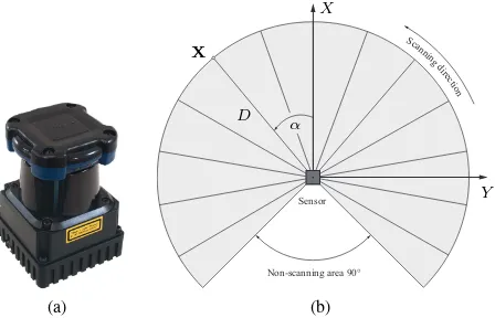
A single-layer LSRF is typically realized as time-of-flight rang-ing system. It uses pulsed laser light beams to directly measure a time delay created by light traveling from the sensor to the object and back. The laser scanning unit measures very fast by send-ing light beams into the center of a continuously rotatsend-ing mir-ror. Latest devices like the 210 gram light-weight Hokuyo UTM-30LX-EW (figure 1a) shift this mirror with an angular resolution of0.25 degbetween each measurement in a few microseconds. With270 degfield of view, the Hokuyo scanner provides 1080 measurements per scan line in 25 ms. The scanning range is 0.1 m to 30 m. Multi-echo functionality allows to receive up to three echoes of a single emitted light pulse.
The spherical coordinates of an object point are given as (D, α, β), whereD is the measured slant range andαthe cor-responding horizontal deflection angle. 2D LSRF take measure-ments over a plane (figure 1b). Consequently, the vertical angle
(a)
Figure 1: (a) Laser scanning range finder Hokuyo UTM-30LX-EW (Hokuyo, 2014). (b) Measuring principle and coordinate sys-tem definition.
Complete 3D scans can be achieved implicitly by moving the platform on which the sensor is mounted. The registration of sin-gle measurement stripes can for example be realized by GPS/INS integration (Maier and Kleiner, 2010), by 3D visual SLAM with a camera (Georgiev and Allen, 2004) or by attaining accurate sen-sor pose with respect to a fixed 3D reference frame (Antone and Friedman, 2007). Considering lever-arm and bore-sight effects finally results in a 3D point cloud representation of the object space. Complete 3D scans can be achieved implicitly by mov-ing the platform on which the sensor is mounted. The registra-tion of single measurement stripes can for example be realized by GPS/INS integration (Maier and Kleiner, 2010), by 3D visual SLAM with a camera (Georgiev and Allen, 2004) or by attaining accurate sensor pose with respect to a fixed 3D reference frame (Antone and Friedman, 2007). Considering lever-arm and bore-sight effects finally results in a 3D point cloud representation of the object space.
ERROR SOURCES AND CALIBRATION STRATEGIES
The measured ranges and angles are used for calculating 3D point cloud coordinates (equation 1). The modeling of deviations from the ideal measurement model is required, if accurate 3D infor-mation should be delivered. A number of systematic and random errors can act on the original observations of a laser scanner: Ef-fects caused by temperature and running-in behavior or multipath propagation can be decreased or even avoided by an adequate measurement setup. The influence of white noise can be com-pensated in static, non-time-critical applications by mean of long-term measurements. Laser beam divergence may cause angular displacement errors depending on the location and the shape of the scanned object. Lichti and Gordon (2004) use a probabilistic model to specify the magnitude of this unpredictable error to be equal to one-quarter of the laser beam diameter. Target properties such as color, brightness and material may also have a significant influence on LSRF measurements (Kneip et al., 2009).
The results of the distance and angular measurements are fur-ther affected by perturbations – caused for example by imper-fections in instrument production – which can be considered in an adequate correction model. Sets of additional parameters for
the geometric calibration of terrestrial laser scanning (TLS) in-struments are investigated in e. g. (Gielsdorf et al., 2004; Lichti, 2007; Schneider and Schwalbe, 2008), general correction models are summarized in (Vosselman and Maas, 2010). The following considerations base on these works.
A linear distance correction term considers a shifta0of the mea-surement origin and a scale variationa1caused by counter fre-quency deviations. A vertical offset of the laser axis from the trunnion axis as well as cyclic distance errors are supposed to be not existent for a 2D single-layer time-of-flight LSRF (section 2). The appropriate distance correction model is defined as
∆D=a0+a1·D (2)
The correction model for errors in horizontal direction consists of six correction terms, namely a horizontal encoder (circle) scale errorb1, two componentsb2, b3for modeling the horizontal circle eccentricity, two further componentsb4, b5for modeling the non-orthogonality of the plane containing the horizontal encoder and the rotation axis and, finally, the eccentricityd6of the collimation axis relative to the rotation axis.
∆α=b1·α
+b2·sinα+b3·cosα+b4·sin 2α+b5·cos 2α
+b6·D− 1
(3)
Further additional parameters to correct the collimation and trun-nion axis errors are not required due to the 2D scanning principle. Also a correction model for errors in elevation angle is not nec-essary.
Several calibration strategies are reported in the literature to cor-rect LSRF errors described above. Ye and Borenstein (2002) or Okubo et al. (2009) for example utilize a computer-controller lin-ear motion table for calibrating the scanner device. The experi-mental configuration is extended in (Kneip et al., 2009) by set-ting not only reference values for the distance measurement, but for the incidence angle as well. Jain et al. (2011) use time domain techniques for error modeling. Kim and Kim (2011) fit cubic Her-mite splines scan-wise to data captured on a translation/rotation stage.
The calibration approaches reviewed above utilize reference stag-es or comparators for accurate translational and rotational dis-placement measurements. Reference values can also be provided indirectly by the network geometry determined in the course of a self-calibration, a procedure which reduces time and instru-mental effort significantly. Self-calibration strategies are well-established for 3D TLS (e. g. Schneider and Maas, 2007; Lichti, 2009). Glennie and Lichti (2010) collect a static data set of planar features in order to determine the internal calibration parameters of a multi-layer LSRF in a bundle adjustment. The further de-velopment for compact and light-weight single-layer 2D LSRF is the main core of this contribution.
INTEGRATED SELF-CALIBRATING BUNDLE ADJUSTMENT
4.1 Geometric Principle
and stochastic context. (3) The future expansion of the mathe-matical model developed is facilitated due to its adaptivity and modular implementation. (4) The method requires only a target field, which is stable, compact, portable as well as easy in set-up and dismantle, but it does not require reference values.
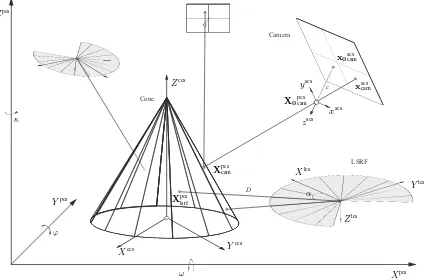
The geometric principle is shown in figure 2. It is based on an in-tegrated self-calibrating bundle adjustment of directional distance measurements of a LSRF. Additional images of a digital single-lens reflex camera (DSLR) ensure a stable network geometry.
The reference between LSRF data and DSLR data can either be realized by identifying homologous points in both data sets (which is quite difficult) or by using easily parametrizable geo-metric primitives (Westfeld and Maas, 2013). In the integrated self-calibrating bundle adjustment presented here, spatial distrib-uted cones functioning as 3D primitives. Their parameters as well as their poses can be determined from both, LSRF and DSLR ob-servations.
The original LSRF measurements(D, α) are transformed into a local laser scanner coordinate system (lcs) using equation 1. The 3D object coordinatesXlcslsrfobtained are subsequently trans-formed into 3D object coordinatesXpcs
lsrfof a higher-level project coordinate system (pcs):
Xpcs
lsrf=X0pcslsrf+mlcspcs·Rpcslcs ·Xlcslsrf (4) where
X0pcslsrf LSRF origin in project coordinate system
mpcslsrf Scale factor
Rpcs
lsrf Rotation matrix
DSLR images of signalized points on target’s surfaces are further captured in order to reliably estimate positions and orientations of the cone primitives. The rule for mapping an image pointxscscam, which is measured in a local sensor coordinate system (scs), into its corresponding object pointXpcscamis
Xpcscam=X0
,lsrf Camera’s projection center mpcsscs Scale factor
Rpcsscs Rotation matrix
In order to set the geometric relation between both sensors, all ob-ject pointsXccslsrf,camin a local cone coordinate system (ccs) deter-mined from LSRF resp. DSLR data should satisfy the following general equation of a cone:
0 = r
rmax Maximum radius on cones bottom hmax Maximum cone height
The necessary transformation between local cone coordinate sys-tem and project coordinate syssys-tem is given by
Xpcs
Xpcs0,cone Cone’s origin in project coordinate system
mpcs
ccs Scale factor
Rpcsccs Rotation matrix
4.2 Functional Model
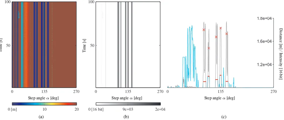
2D LSFR: LSRF directly deliver distance and angular obser-vations as well as intensity information. The task is to automate the detection of the cones in each scan line at each position. An analysis of both intensity and range data is performed to identify all measurement points belonging to a reference primitive (fig-ure 3c). In detail, the processing chain consists of the following steps:
1. Calculate the mean of the long-term measurements (figures 3a and 3b) performed at each position and further smooth the resulting single scan lines by moving average (figure 3c; cyan and black graphs).
2. Apply dynamically derived distance and intensity thresholds for further data containment.
3. Find local maxima to roughly detect the positions of the cones (figure 3c; red crosses).
4. Calculate local extrema of distance gradient curves.
5. All measurement points located between two local extrema belong to a cone if and only if a rough cone position detected in (3) is included (figure 3c; red dotted lines).
6. Remove outliers, for instance caused by multipath effects at surface edges.
The distances measured between LSRF optics and cone surfaces serve as first, the corresponding angles of deflection as second observation type:
The observation equations 8 and 9 include the unknown distance and angular error-correction parameters∆D resp. ∆α intro-duced in section 3.
Further unknowns are the 3D coordinates of each scanned point on the cone surfaces, in a first instance as local sensor coordinates
Xlcslsrf. Using equation 4 results in higher-level project coordinate
Xpcs
lsrfwhich have to fulfill the constraint equation 6 including the unknown cone parameters radiusrmaxand heighthmax.
The fact that a 2D LSRF measures in one horizontal laser scan-ner plane only has taken into account by the following constraint which forces the vertical angleβto be zero:
β= arctan Z
Camera
c
LSRF
D Cone
ω ϕ
κ
α
Xpcs Ypcs
Zpcs
Xccs Y
ccs Zccs
xscs yscs
zscs
x0scscam
xscscam
X0pcscam
Xpcscam
Xpcs
lsrf
Xlcs
Ylcs
Zlcs
Figure 2: Geometric model.
corresponding observation equations for mapping an object point
Xpcscam(X, Y, Z)to an image pointxscs
cam(x, y)using a central pro-jection:
x=x0
−c·r11·(X−X0) +r21·(Y −Y0) +r31·(Z−Z0)
r13·(X−X0) +r23·(Y −Y0) +r33·(Z−Z0)
+ ∆x y=y0
−c·r12·(X−X0) +r22·(Y −Y0) +r32·(Z−Z0)
r13·(X−X0) +r23·(Y −Y0) +r33·(Z−Z0)
+ ∆y
(11)
where
c Focal length
x0 Principal point ∆x Correction functions
X0 Projection center
rr,c Elements of a rotation matrixR
The unknowns which can be estimated from equation 11 are the focal lengthc, the principal pointx0 and the parameters of the image correction functions∆xas interior orientation parameters as well as the exterior orientation parameters X0
pcs cam and
Rpcsscs(ω, ϕ, κ)of the supporting DSLR camera. Further, the
coor-dinatesXpcscam(X, Y, Z)of all object points signalized on the cone surfaces can be calculated in project coordinate system. Like the 3D coordinates determined by the LSRF, they should also satisfy the general equation 6 of a cone.
Additional Constraints: A 3D rotation can be described by three Euler angles(ω, ϕ, κ)or, in order to avoid ambiguous trig-onometric functions, by four quaternions(q1, q2, q3, q4). The use of quaternions makes sense from a numerical point of view, but requires one additional equation per LSRF resp. DSLR position
Figure 4: Image point coordinate measurement by ellipse fit.
to enforce an orthogonal rotation matrixR:
1 =q21+q 2 2+q
2 3+q
2
4 (12)
The reference frame of the integrated self-calibrating bundle ap-proach should be adjusted as an unconstrained network. The rank defect of the resulting singular system of equations can be re-moved by including seven additional constraints: 3 translations, 3 rotations, 1 scaling factor, (e. g. Luhmann et al., 2006). The scale was determined by two diagonal reference distances across the target field and used to fix the scale factorsmpcs
within the transformation equations 4, 5 and 7.
4.3 Stochastic Model
0 135 270 100
50
0 [m] 10 20
Step angleα[deg]
T
Step angleα[deg]
T
Step angleα[deg]
D
Figure 3: Part of (a) range and (b) intensity LSRF raw data captured from one position over time. The five bluish/black lines in range/intensity data (in a distance of approx. 5 maround the region of135 deg) clearly represent the five cones. The result of the segmentation of the cones is shown in (c): The cyan and the black curves represent the mean of the long-term measurements in distance resp. intensity channel. The red crosses roughly mark the detected cone positions, and the red lines highlight the corresponding measurement points which are introduced into the bundle adjustment.
with unknown accuracy as well as different constrained geomet-ric relations. The expansion of the stochastic model to the geode-tic concept of include variance component estimation (VCE; Ku-bik, 1967; F¨orstner, 1979) ensures that this heterogeneous infor-mation pool is fully exploited.
The stochastic model is represented by the variance-covariance matrix Σll of the observations before the adjustment process. The weights of the observations are given by the quotient ofs2 0 tos2
i. The variance of the unit weights 2
0is a constant, andsiare the variances of the observations, namely the variance compo-nents2
Dfor the LSRF distance measurements,s 2
αfor tapping the LSRF deflection angles ands2
xyfor the DSLR image point mea-surements. To differentiate between constant and distance-related error components, the group variance for the distance measure-ment is further separated into two adaptive variance components
s2
(Sieg and Hirsch, 2000).Σllcan now be subdivided into three components, i.e., one (adaptive) component per group of observation:
Σll=diag(ΣD,Σα,Σxy)
The remaining additional constraints for the non-existent vertical angle (equation 10), the implementation of quaternions (equation 12) as well as for a free network adjustment are considered to be mathematically rigorous byPC =0in the extended system of normal equations (Snow, 2002; section 4.4). Solely the geomet-ric cone model is introduced less restgeomet-rictive due to imperfections in the manufacturing of the traffic cones, which were used as ref-erence primitives (equation 6; section 5.1). Their weights are adjusted automatically as fourth variance component group.
In the course of the VCE, the approximate values for the variance components are improved within a few iterations. See (Koch, 1999) for further information.
4.4 Solving the Adjusmtent Task
The integrated bundle adjustment bases on an extended Gauss-Markov model:
The functional model (section 4.2) is required to set up the coeffi-cient matricesAandB, which contain the linearized observation and constraint equations, the reduced observation vectorland the
vector of inconsistenciesw. The weight matricesPandPCas inverse variance-covariance matricesΣll resp. ΣC define the stochastic model (section 4.3). The extended system of normal equations is solved iteratively. At each step, the solution vectorˆx
is added to the approximate values of the previous iteration until the variances reach a minimum and the optimization criterion is fulfilled.
As a least squares adjustment, the method delivers information on the precision, determinability and reliability of the unknown parameters. This includes the a-posteriori variances2
i of each of the parameters as well as the correlation between parameters. In combination with an automatic VCE, a-posteriori variancess2 l ands2
ˆ
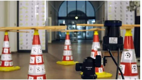
Figure 5: Measuring device Hokuyo UTM-30LX-EW in front of the target field.
RESULTS
5.1 Experimental Configuration
A 3D calibration target field was designed in order to proof the concept presented here (figure 5). It consists of eight standard retro-reflective traffic cones with a maximum height hmax of
90 cm and a maximum radius rmax of 15 cm. The cones are spatial distributed over an area of approximately10 m×5 m. Six LSRF positions in distances of up to15 mallow for the de-termination of all distance- and angular-related correction terms. LSRF scans in larger distances could not be oriented reliably. The 3D target field was further captured by a supporting DSLR cam-era. Overall 100 convergent images, some of them rolled against the camera axis, ensure a stable network geometry.
5.2 LSRF Calibration Parameters
Table 1 lists the LSRF calibration parameters and the correspond-ing a-posteriori standard deviations estimated within the integrat-ed bundle adjustment. The additive terma0of the distance cor-rection model ∆D is 9 mm, the multiplicative parameter a1 amounts to 0.19 % of the measured distance. The circle scale
b1 to correct errors in horizontal direction is -0.21 % of the de-flection to the zero point. The eccentricity of the collimation axis to the rotation axis causes a correction of up to 3.5 mm. Further parameters of the correction model∆αfor errors in horizontal direction could not be estimated significantly.
Considerable correlations between the LSRF calibration terms could not be observed. The highest coefficient is about0.7 be-tween the distance correction parametersa0anda1.
5.3 LSRF Pose
The pose of a single LSRF view point can be stated with an a-posteriori RMS of1.7 mmresp. 7.2 mmfor the position of the projection center in xy- resp. z-direction of the project coordinate system. The mean RMS deviation of the rotation components is 0.14 deg. The uncertainties in determining LSRF height com-ponents can be explained by the unfavorable ratio between the maximum radius and the height of the traffic cones used.
5.4 Cone Parameters and Pose
The parameters as well as the poses of the cone primitives are estimated by directional LSRF distance measurements and DSLR image coordinate measurements. The unknown cone parameters are calculated with a RMS error of 0.5 mm for a maximum radius of 14.34 cm and 8.8 mm for a height of 90.13 cm, and the poses with a mean a-posteriori standard deviation of 0.11 mm for the shift and9.46e−3degfor the rotation.
5.5 3D Object Coordinates
The mean a-posteriori standard deviation of the cone surface pointsXlsrf observed by the LSRF is4.8 mmin lateral direc-tion and9.2 mmin height. The precision of a 3D object point
Xcamestimated from DSLR image coordinate measurements is 0.09 mm.
5.6 Residuals
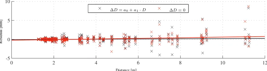
The residualsvDof the distance measurements are shown in fig-ure 7 for an adjustment with and without considering the LSRF error correction model. The red graph results from of a func-tion fitted into the residuals of the uncorrected distance measure-ments. It indicates a slight constant offset and a distance-related trend. The RMS of the residuals is0.63 mm, the expected value µ is -0.28 mm. The black graph of a function fitted into the remain-ing residuals after a adjustment parametrized with LSRF correc-tion terms is nearly a straight line withy = 0 = const. The normally distributed residuals do not show interpretable effects. The RMS is equal to the previous solution, but the expected value µ= 0.8µmtends more clearly towards zero.
The situation is similar for the residuals of the angular measure-ments: The RMS of the angular residuals of an un-parametrized estimation is0.1 deg(µ = 2.52e−2deg). If calibration param-eters are taken into account, the RMS is reduced to 0.06 deg (µ= 9.05e−3deg).
The normally distributed residualsvxy of the image coordinate measurements do not show any systematic effect. They vary in both coordinate directions with an a-posteriori RMS deviation
svxyabout1/20pixelaround the expected value µ= 1.7e−3µm. Even though probably not all LSRF effects are considered, the results show that the integration of LSRF correction parameters is better suited to model the geometric-physical reality of a LSRF measurement process.
5.7 Observational Errors
The a-posteriori standard deviations of the original observations estimated automatically by VCE as well as of the adjusted ob-servations calculated in the course of the error analysis after the bundle adjustment are shown in table 2.
ˆ
sD0 ˆsD1 ˆsα sˆxy
not significant 1.95e−3 3.46e−3rad 0.57µm ˆ
sDˆ ˆsαˆ sˆˆxyˆ
1.47 mm 2.39e−3rad 0.19µm
Table 2: A-posteriori standard deviationsˆsof the original and the adjusted observations.
The deviationˆsD of an original LSRF distance measurement is about0.20 %of the measured distanceD. Depending on the measuring range[1,15 m]specified in section 5.1, the accuracy can thus be stated with[2.0,30 mm]. These values correspond to the level of precision specified by the manufacturer (Hokuyo, 2014). Remark that the constant offsetsˆ2
0 2
4
-14 -12
-10 -8
-6 -4
-2 0
1 2
Xpcs Ypcs
Z
p
c
s
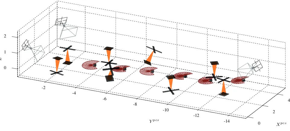
Figure 6: Network geometry: All eight traffic cones and six LSRF positions (represented as fans) are shown, but only a few camera poses for reasons of clarity. The crosses on top as well as the different orientations of the cones additionally ensure a stable network geometry.
a0
(mm)
a1 b1 b2 b3 b4 b5 b6
(mm) ˆ
xi 8.62 1.89e−
3
−2.10e−3 0 0 0 0 3.32 ˆ
sxˆi 1.09 3.54e
−4 3.87e−4 fix fix fix fix 1.64 Table 1: LSRF calibration parametersxˆiwith their standard deviationssˆxˆi.
only be explained by an excessive distance-related influence of the beam divergence on the measurement precision of a Hokuyo UTM-30LX-EW (for more detail see paragraph below).
The deflection angleαis specified with an a-priori standard de-viation of0.2 deg, which corresponds to3/4of the angular step width. This order of magnitude seems to be quite high. One reason for this might be found in the beam divergence. Accord-ing to manufactures information, the elliptical laser spot size of the Hokuyo UTM-30LX-EW is 50 mm×500 mmat sensor’s maximum distance of30 m. This footprint corresponds to an an-gular widening of approximately0.1 deg×1.0 deg. Further, the orientation of the laser spot (in scan direction resp. across scan direction) depends on the deflection angle and alternates within a single scan line.
In average, the a-posteriori standard deviationˆsxy of an image coordinate measurement is 1/15pixel. It is thus slightly worse than the precision of the pure image point measurement by ellipse fit as stated in section 4.2.
The a-posteriori standard deviationˆs0of the unit weight is near to the a-priori constant values0 = 100, which indicates an op-timally determined accuracy ratio for all groups of observations. This implies that the a-posteriori variances of the original obser-vations are equal to their a-priori variances.
The mean standard deviationssˆDˆ andˆsαˆ of the adjusted LSRF observations are 1.5 mm for the distance measurement and 0.1 degfor the angular values. In average, the a-posteriori stan-dard deviationˆsxˆyˆof an image coordinate measurement becomes 1/43pixel.
CONCLUSION AND OUTLOOK
The flexible self-calibrating bundle adjustment approach present-ed in this contribution determines a geometric correction model of a 2D single-layer LSRF and estimates all distance- and angular-related correction parameters. The heterogeneous infor-mation pool is fully exploited by estimating variance components automatically within the integrated stochastic model. The experi-mental configuration of the self-calibration is based on a portable 3D target field, whose geometry is determined simultaneously in the adjustment. Complex experimental set-ups can thus be avoided.
The process validation showed that the integration of LSRF cal-ibration parameters leads to a more accurate solution. The accu-racy of an original LSRF range measurement can be stated with approximately0.2 %of the measured distance and with0.2 deg for the angle specifications. The RMS error of a 3D coordinate after the calibration becomes5 mmin lateral and9 mmin depth direction.
0 2 4 6 8 10 12 -5
0 5 10
Distance [m]
R
es
id
u
al
[m
m
]
∆D=a0+a1·D ∆D= 0
Figure 7: Residuals of the distance measurements with (black) and without (red) correction parameters.
ACKNOWLEDGEMENTS
The research work presented in this paper has been funded by the European Social Fund (ESF) via S¨achsische Aufbaubank (SAB).
References
Antone, M. E. and Friedman, Y., 2007. Fully automated laser range calibration. In: BMVC, British Machine Vision Associ-ation.
Djuricic, A. and Jutzi, B., 2013. Supporting uavs in low visi-bility conditions by multiple-pulse laser scanning devices. In: C. Heipke, K. Jacobsen, F. Rottensteiner and U. S¨orgel (eds), High-resolution earth imaging for geospatial information. In-ternational Archives of Photogrammetry, Remote Sensing and Spatial Information Sciences, Vol. XL-1/W1, pp. 93–98.
F¨orstner, W., 1979. Ein Verfahren zur Sch¨atzung von Varianz- und Kovarianzkomponenten. Allgemeine Vermes-sungsnachrichten 86, pp. 41–49.
Georgiev, A. and Allen, P. K., 2004. Localization methods for a mobile robot in urban environments. IEEE Transactions on Robotics 20, pp. 851–864.
Gielsdorf, F., Rietdorf, A. and Gruendig, L., 2004. A concept for the calibration of terrestrial laser scanners. In: Proc. of FIG Working Week, Athens, Greece.
Glennie, C. and Lichti, D. D., 2010. Static calibration and analy-sis of the velodyne hdl-64e s2 for high accuracy mobile scan-ning. Remote Sensing 2(6), pp. 1610–1624.
Hokuyo, 2014. Product Information UTM-30LX-EW. Hokuyo Automatic Co., Ltd., Japan.
Holz, D., Nieuwenhuisen, M., Droeschel, D., Schreiber, M. and Behnke, S., 2013. Towards multimodal omnidirectional obsta-cle detection for autonomous unmanned aerial vehiobsta-cles. ISPRS - International Archives of the Photogrammetry, Remote Sens-ing and Spatial Information Sciences XL-1/W2, pp. 201–206.
Jain, S., Nandy, S., Chakraborty, G., Kumar, C., Ray, R. and Shome, S., 2011. Error modeling of laser range finder for robotic application using time domain technique. In: IEEE In-ternational Conference on Signal Processing, Communications and Computing (ICSPCC), pp. 1 – 5.
Kim, J.-B. and Kim, B.-K., 2011. Efficient calibration of infrared range finder pbs-03jn with scan-wise cubic hermite splines for indoor mobile robots. In: 8th International Conference on Ubiquitous Robots and Ambient Intelligence (URAI), IEEE, pp. 353–358.
Kneip, L., Tˆache, F., Caprari, G. and Siegwart, R., 2009. Charac-terization of the compact hokuyo urg-04lx 2d laser range scan-ner. In: IEEE International Conference on Robotics and Au-tomation, IEEE, pp. 1447–1454.
Koch, K.-R., 1999. Parameter estimation and hypothesis testing in linear models. Springer.
Kr¨uger, T., Nowak, S., Matthaei, J. and Bestmann, U., 2013. Single-layer laser scanner for detection and localization of un-manned swarm members. ISPRS - International Archives of the Photogrammetry, Remote Sensing and Spatial Information Sciences XL-1/W2, pp. 229–234.
Kubik, K., 1967. Sch¨atzung der Gewichte der Fehlergleichungen beim Ausgleichungsproblem nach vermittelnden Beobachtun-gen. Zeitschrift f¨ur Vermessungswesen 92, pp. 173–178.
Kuhnert, K.-D. and Kuhnert, L., 2013. Light-weight sensor pack-age for precision 3d measurement with micro uavs e.g. power-line monitoring. ISPRS - International Archives of the Pho-togrammetry, Remote Sensing and Spatial Information Sci-ences XL-1/W2, pp. 235–240.
Lichti, D. D., 2007. Error modelling, calibration and analysis of an am–cw terrestrial laser scanner system. {ISPRS}Journal of Photogrammetry and Remote Sensing 61(5), pp. 307 – 324.
Lichti, D. D., 2009. Terrestrial laser scanner self-calibration: Correlation sources and their mitigation. ISPRS Journal of Photogrammetry and Remote Sensing 65(1), pp. 93–102.
Lichti, D. D. and Gordon, S. J., 2004. Error propagation in di-rectly georeferenced terrestrial laser scanner point clouds for cultural heritage recording. In: Proc. of FIG Working Week, Athens, Greece.
Luhmann, T., Robson, S., Kyle, S. and Harley, I., 2006. Close Range Photogrammetry: Principles, Methods and Applica-tions. Revised edition edn, Whittles Publishing.
Maier, D. and Kleiner, A., 2010. Improved gps sensor model for mobile robots in urban terrain. In: ICRA, IEEE, pp. 4385– 4390.
Nowak, S., Kr¨uger, T., Matthaei, J. and Bestmann, U., 2013. Mar-tian swarm exploration and mapping using laser slam. ISPRS - International Archives of the Photogrammetry, Remote Sens-ing and Spatial Information Sciences XL-1/W2, pp. 299–303.
Rogers III, J. G., Trevor, A. J., Nieto-Granda, C., Cunningham, A., Paluri, M., Michael, N., Dellaert, F., Christensen, H. I. and Kumar, V., 2010. Effects of sensory precision on mobile robot localization and mapping. In: Experimental Robotics, Springer, pp. 433–446.
Scherer, S., Rehder, J., Achar, S., Cover, H., Chambers, A. D., Nuske, S. T. and Singh, S., 2012. River mapping from a flying robot: state estimation, river detection, and obstacle mapping. Autonomous Robots 32(5), pp. 1 – 26.
Schneider, D. and Maas, H.-G., 2007. Integrated bundle adjust-ment of terrestrial laser scanner data and image data with vari-ance component estimation. The Photogrammetric Journal of Finland 20, pp. 5–15.
Schneider, D. and Schwalbe, E., 2008. Integrated processing of terrestrial laser scanner data and fisheye-camera image data. International Archives of Photogrammetry, Remote Sensing and Spatial Information Science 37, pp. 1037–1044.
Serranoa, D., Uijt de Haag, M., Dill, E., Vilardaga, S. and Duan, P., 2014. Seamless indoor-outdoor navigation for unmanned multi-sensor aerial platforms. ISPRS - International Archives of the Photogrammetry, Remote Sensing and Spatial Informa-tion Sciences XL-3/W1, pp. 115–122.
Sieg, D. and Hirsch, M., 2000. Varianzkomponentensch¨atzung in ingenieurgeod¨atsichen Netzen, Teil 1: Theorie. Allgemeine Vermessungsnachrichten 3, pp. 82–90.
Snow, K. B., 2002. Applications of Parameter Estimation and Hypothesis Testing of GPS Network Adjustments. Technical Report 465, Geodetic and GeoInformation Science, Depart-ment of Civil EnvironDepart-mental Engineering and Geodetic Sci-ence, The Ohio State University, Columbus, Ohio, USA.
Vosselman, G. and Maas, H.-G. (eds), 2010. Airborne and Ter-restrial Laser Scanning. Whittles Publishing, Caithness, UK.
Westfeld, P. and Maas, H.-G., 2013. Integrated 3d range cam-era self-calibration. PFG Photogrammetrie, Fernerkundung, Geoinformation 2013(6), pp. 589–602.