ENTROPY BASED DETERMINATION OF OPTIMAL PRINCIPAL COMPONENTS OF
AIRBORNE PRISM EXPERIMENT (APEX) IMAGING SPECTROMETER DATA FOR
IMPROVED LAND COVER CLASSIFICATION
Akhil Kallepalli a, *, Anil Kumar a and Kourosh Khoshelham b
a, * Indian Institute of Remote Sensing (Indian Space Research Organization), Dehradun, India – [email protected] a Indian Institute of Remote Sensing (Indian Space Research Organization), Dehradun, India – [email protected]
b Faculty of Geo-Information Science and Earth Observation (ITC), University of Twente, The Netherlands – [email protected]
KEY WORDS: High resolution data, hyper spectral, land cover, classification, feature extraction
ABSTRACT:
Hyperspectral data finds applications in the domain of remote sensing. However, with the increase in amounts of information and advantages associated, come the „curse‟ of dimensionality and additional computational load. The question most often remains as to which subset of the data best represents the information in the imagery. The present work is an attempt to establish entropy, a statistical measure for quantifying uncertainty, as a formidable measure for determining the optimal number of principal components (PCs) for improved identification of land cover classes. Feature extraction from the Airborne Prism EXperiment (APEX) data was achieved utilizing Principal Component Analysis (PCA). However, determination of optimal number of PCs is vital as addition of computational load to the classification algorithm with no significant improvement in accuracy can be avoided. Considering the soft classification approach applied in this work, entropy results are to be analyzed. Comparison of these entropy measures with traditional accuracy assessment of the corresponding „hardened‟ outputs showed results in the affirmative of the objective. The present work concentrates on entropy being utilized for optimal feature extraction for pre-processing before further analysis, rather than the analysis of accuracy obtained from principal component analysis and possibilistic c-means classification. Results show that 7 PCs of the APEX dataset would be the optimal choice, as they show lower entropy and higher accuracy, along with better identification compared to other combinations while utilizing the APEX dataset.
* Corresponding author. This is useful to know for communication with the appropriate person in cases with more than one author.
1. INTRODUCTION
“Remote sensing is the science and art of obtaining information about an object, area, or phenomenon through the analysis of data acquired by a device that is not in contact with the object, area, or phenomenon under investigation” (Lillesand, Kiefer, and Chipman). Of the many types of remote sensing, hyperspectral remote sensing has emerged as one of the most active areas of research (Qian and Chen 2007). A distinctive advantage of imaging spectroscopy is data acquisition across contiguous spectral bands, which in turn allows a focussed analysis of objects (and specific properties) on the ground.
Hyperspectral remote sensing (or imaging) enables analysis of greater spectral detail and variations of targets (da Silva, Centeno, and Aranha 2008) as compared to multi-spectral data. But with higher spectral detail, the problem of dimensionality and increase in computational load is commonly associated. The dimensionality problem affects the classification of raw hyperspectral data and is known as “Hughes Phenomenon” (Hughes 1968). Hughes describes this “peaking paradox” as the achieving of a optimal value of statistical recognition accuracy with a subset of bands and subsequent declination due to inadequate training samples. Evidence of reduction in computational load was also found when dimensionality of the data was reduced (da Silva, Centeno, and Aranha 2008). Successful studies have been carried out to reduce dimensionality of hyperspectral data (Qian and Chen 2007; Harsanyi and Chang 1994; Plaza et al. 2005), before further processing and analysis of hyperspectral data.
Remote sensing is essentially completed in three steps; (i) data acquisition; (ii) image processing and (iii) interpretation process (Dehghan and Ghassemian 2006). All the techniques in the mentioned stages are prone to uncertainty (Giles M. Foody and Atkinson 2002; Dehghan and Ghassemian 2006). Entropy provides a method to study and understand the variation of uncertainty in classification outputs. The measure of degree of uncertainty of classification results assist in evaluating the classifier performance, thereby indirectly providing a measure of how accurately a pixel of a certain class is assigned to the corresponding label (Dehghan and Ghassemian 2006; Kumar and Dadhwal 2010).
The primary objective of this work is to understand the dimensionality of hyperspectral datasets, and post classification of principal component databases, to establish entropy as an acceptable measure for choice of optimal principal components from the dataset.
2. LITERATURE BACKGROUND
Vane and Goetz (1988) (Vane and Goetz 1988) published a comprehensive analysis of imaging spectroscopy, emerging as a new approach of Earth remote sensing. A review of multi- and hyperspectral imaging was given by Govender et al., 2007 (Govender, Chetty, and Bulcock 2007), with focus on hyperspectral imagery applications. A multitude of applications have been widely researched. The goal of hyperspectral image processing is to detect and classify every pixel in the scene and The International Archives of the Photogrammetry, Remote Sensing and Spatial Information Sciences, Volume XL-8, 2014
reduce the dimensionality without loss of critical information (Harsanyi and Chang 1994). Most linear transformations like Principal Component Analysis (PCA) (Rodarmel and Shan 2002), etc. have been used to counter the „curse‟ of dimensionality (Hughes 1968).
Although the approach by Hughes, to define the curse of dimensionality, was criticised and stated as an „apparent paradox‟ by researchers like Van Campenhout (Van Campenhout 1978), the curse of dimensionality stands as a complication of high spectral resolution. Considered in this study is a highly accepted method of dimensionality reduction, i.e. PCA (Jolliffe 2002). Detailed explanations of the data transformations associated with this method of feature extraction are given by Rodarmel and Shan (Rodarmel and Shan 2002). PCA calculates orthogonal projections that maximize variance in data, yielding data in a new uncorrelated coordinate system (Plaza et al. 2005). Reduction in computational duration and increase in accuracy assessment provides adequate proof that PCA is an effective pre-processing step for hyperspectral data analysis.
Traditional methods of remote sensing supervised classification, training information and results are depicted in the one-pixel-one-class method (Wang 1990). As class mixing cannot be taken into consideration while training „hard‟ classifiers, this limitation has reduced classification accuracy. The work by Wang (1990) supports the applicability of fuzzy based classification techniques against conventional “one -pixel-one-class” methods. The fundamental drawback of all such classification techniques is that most spectral information is lost in the process of transforming the remotely sensed data to generate a thematic map (Foody et al. 1992). Foody (2004) (Giles M. Foody 2004) details the many sub-pixel methods in remote sensing. Considering that data is obtained in varying spectral and temporal resolutions, many accurate methods of classification have been researched and published. However, this doesn‟t change the fact that, in practice, absolute accurate classification of land cover is a difficult task (Townshend 1992). It is important to note that use of fine spatial resolution data does not necessarily eliminate the problem of mixed pixels, as the class‟s constituent parts may carry importance and fine resolution data over large regions is impractical. In the case of soft classification approaches, pixels are not „forced‟ to show full membership (or belonging) to a single class. Thus, the contribution of classes to a single pixel is measured in terms of membership values that define the degree of the pixel belonging to a specific class. Outputs of soft classification are also derived similar to linear unmixing, i.e. a fraction image corresponding to each class (Kumar and Dadhwal 2010). Of the many sub-pixel classification approaches, in the present context, Possibilistic c-means algorithm is considered as the membership values derived are “measures of the absolute strength of class membership” (R. Krishnapuram and Keller 1993; Raghuram Krishnapuram and Keller 1996; Giles M. Foody 2004) and not influenced by presence of untrained classes, making in feasible in cases where the classes may not be exhaustively defined.
Entropy provides a method to study and understand the variation of uncertainty in classification outputs. Mathematically, entropy expresses the amount of statistical information of a system described by N discrete levels (Maselli, Conese, and Petkov 1994). Entropy is evaluated from the membership vector of a pixel. The membership vector (µ (P/x)) of a pixel is the membership value of a pixel in each of the classes‟ fraction outputs.
(1)
Where µ (P/x) is the membership vector; of class “k” for pixel
“x” for “C” classes.
Entropy is a criterion that summarizes the classification uncertainty in a single number, per pixel, per class or per image (Dehghan and Ghassemian 2006). It calculated, while utilizing the PCM algorithm, using Eq. 2:
(2)
Maselli et al., 1994 (Maselli, Conese, and Petkov 1994) discusses the applicability of entropy for estimation of accuracy of soft ML classification. The ML classifier using non-parametric priors yielded a high accuracy, supported by low entropy values. There is a requirement of fuzzy ground data as compared to the traditionally used hard ground truth data to assess the accuracy of fuzzy classification (Giles M. Foody 1995).
3. DATASET AND STUDY AREA
The need for a flexible hyperspectral mission against competing systems like CASI (Compact Airborne Spectrographic Imager), GERIS (Geophysical Environment Research Imaging Spectrometer) and DAIS (Digital Airborne Imaging Spectrometer) (Itten et al. 2008) prompted the Airborne Prism EXperiment (APEX) project. Co-funded by Switzerland and Belgium, the APEX instrument operates between 380 and 2500 nm in 313 freely configurable bands (Itten et al. 2008; Jehle et al. 2010). Detailed information regarding the ESA-APEX program, sensor characteristics and other information can be found in (Schlapfer et al. 2000; Itten et al. 2008) and (Hueni et al. 2009). The APEX Open Science Dataset (OSD) (Itten et al. 2008; Jehle et al. 2010) was acquired in June 2011. After extensive calibration and pre-processing of the raw data to Level1 processed data (“APEX Open Science Data Set Leaflet” 2011), the dataset is made available on the website,
http://www.apex-esa.org/content/free-data-cubes (“APEX”
2013), as Open Science Dataset with a spectral resolution of 285 bands and spatial resolution of 1.8 meters, in RAW (imaging geometry), ENVI cube format.
Although the focus is on the dataset in this study, it is important to understand the diversified land cover classes in the image. These classes range from roads, roofs and other urban features to a multitude of vegetation classes like grass and forest. Ground truth information and class sites are vital for (i) Training the classifier; (ii) Entropy calculations; and (iii) Testing the classification results.
The classes were identified from interpretations from SwissTopo web portal (“SwissTopo Web Portal” 2014). Regions of Interest (ROIs) were collected, verified with the data providers and used for classification and accuracy analysis. The International Archives of the Photogrammetry, Remote Sensing and Spatial Information Sciences, Volume XL-8, 2014
Figure 1 - True Colour Composite of APEX Open Science Dataset
4. METHODOLOGY
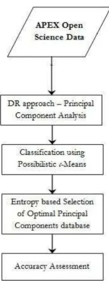
The data is interpreted in terms of classes constituted in the study area and identification of vital training and testing data sites. Due to the high spectral resolution of the hyperspectral dataset, a very detailed spectral response curve analysis can be made of the classes (or object classes) on the ground. Besides the high spectral resolution (of 285 bands), the dataset has a fine spatial resolution of 1.8 meters. The adopted methodology is illustrated in Figure 3.
The object classes identified in the study area are:
1. Artificial Turf 2. Black Roof 3. Building 4. Clay Soil 5. Grass
6. Lawn Tennis Court 7. Mixed Coniferous Forest 8. Mixed Deciduous Forest 9. Pasture
10. Railway 11. Red Roof
12. Red Synthetic Ground 13. Road
14. Roofs 15. Sand
16. Stressed Grass
17. Synthetic Sports Surface 18. Vineyard
19. Water 20. Yellow Tartan
Feature extraction algorithms create new features based on transformations of the original feature set (Jain and Zongker
1997). Principal Component Analysis (PCA) is one the most important and widely used method of reducing the dimensionality of data. It produces new attributes/features through linear combinations of the original feature set, orthogonal to each other and quantifies the variation in the data (Janecek and Gansterer 2008). These new features are called Principal Components (PCs). The four main properties/ advantages of PCA are:
1. The features have 0 covariance;
2. Output features are ordered in descending order with respect to variance or amount of data;
3. First output feature contains the maximum amount of information (maximum variance of data);
4. Each successive feature captures as much variance of data as possible (information).
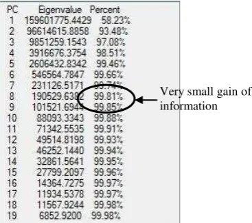
The principal components are generated, displaying the respective Eigen values and percentages of information contained in the respective components (Figure 2). Depending on the amount of information and lack of gain of variance in the increasing PCs, the initial intrinsic dimensionality is reduced to 8 components.
Figure 2 - Percentage depiction of gain in variance with increase in PCs
However, the optimal components were determined from the results of the corresponding classifications. The combination of optimal number of PCs is achieved using entropy, and verified in comparison with accuracy assessment through traditional methods. The inputs to the classifier considered are (PC1), (PC1 and PC2), (PC1, PC2 and PC3)..., (PC1, PC2 ... PC8). The result of adding one PC at a time to the input helps understand which combination of PCs is an optimal choice.
Considering the fact that the classification approach remains the same for each of the inputs, the assessment of Entropy (as a measure of degree of uncertainty) and Accuracy assessment (as a measure of degree of correctness) would be an interpretation of the influence of the input database of PCs. The outputs of the classification process are individual, grey-scale class soft outputs. The successful classification of an object class was assessed by a method of mean difference calculations (Figure 4).
Very small gain of information The International Archives of the Photogrammetry, Remote Sensing and Spatial Information Sciences, Volume XL-8, 2014
Figure 3 - Methodology
The illustration depicts a choice of random pixels in known class locations and calculating the difference in pixel value. If the difference is significant, it implies that the class is separable after classification. If a certain class has been successfully classified, entropy measures and accuracy assessment are attempted to quantify their accuracy of identification. Generalizing, the particular class shows a better contrast in the output with reference to other classes.
Figure 4 - Illustration of class differentiation from soft outputs
Entropy calculations define the degree of certainty with which the classifier assigns a class label to a certain pixel. However, measures of entropy should be supported with accuracy assessment for acceptable interpretations (Giles M. Foody 1995). The entropy measures of the classes are established
using 50-75 membership vectors, depending on the spatial extent of the classes. Defuzzification of the 20 soft outputs was done by a simple maximum value approach. The algorithm reads the membership values along the pixel vector and assigns the class with the maximum membership to the pixel. The combination of 20 soft outputs, each corresponding to its respective class, is “hardened” to a single output, containing classification results that can be evaluated by traditional methods of accuracy assessment (user‟s and producer‟s accuracy), using a combination of user-defined and randomly generated test sites.
5. RESULTS AND DISCUSSIONS
PCA has been used a pre-processing step to classification wherein the algorithm transforms the data into orthogonal projections that maximize variance using linear transformations. The choice of optimal PCs is based on three aspects:
1. Amount of information contained in the principal components;
2. Number of classes successfully identified in the classification output;
3. Minimal entropy (degree of uncertainty).
Figure 2 illustrates the amount of information gained with addition of each principal component. As observed, the amount of information gained beyond the 8th component becomes highly trivial. With a gain of 0.04%, adding dimensions becomes questionable. Therefore, combinations using 8 PCs were considered for further analysis. Each of the PCs is individually added to 1 PC, thereby making the inputs (1PC), (1PC, 2PC), (1PC, 2PC, 3PC)... (1PC, 2 PC ... 8PC). An optimal PCs input would show the maximum number of successful classes identified and comparatively minimal entropy. The corresponding accuracy of the PCs will serve as a supporting factor for entropy.
Figure 5 provides a graphical illustration of classes identified (X axis) with their corresponding entropy values (Y axis). Note that the classes are in the order of identification with respect to increasing PCs input. Therefore, for example, “Lawn Tennis Court” and “Buildings” classes were identified after adding 7 and 8PCs respectively to the input principal components database. “Clay Soil” was successfully identified from the initial considered 3 PCs. An input of the first or first two PCs was not considered as the 2-dimensional signature vector could not distinguish most of the classes, resulting in uninterpretable outputs. Even in the absence of considering the maximum number of classified classes, the entropy values show significantly higher values for classes like “Mixed Coniferous Forest (MCF)” while considering lesser PC inputs.
With reference to previously defined criteria for choice of optimal PCs, maximum number of classes (9) were successfully classified (Figure 5) while considering an input of 7PCs and 8PCs. Considering the individual soft outputs and thresholds of membership values were used to analyze the conflicting classes. The International Archives of the Photogrammetry, Remote Sensing and Spatial Information Sciences, Volume XL-8, 2014
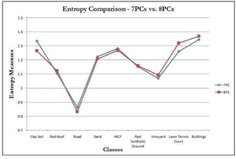
A comparative analysis of entropy values for 7PCs and 8PCs (Figure 6) was approached to determine the optimal PCs. Similar or lesser entropy can be associated with 7PCs input when compared to 8PCs (Figure 6). Therefore, the optimal PCs input is decided to be 7PCs as there is no significant variation in entropy measures with increasing dimensionality of the principal components input. A combination of amount of information in components, number of classes determined and entropy values are, therefore, used to determine the 7PCs as the optimal choice from the initial PCA output.
Also supporting this assessment is the defuzzified evaluation of 8PCs classification output, wherein an accuracy of 57.50% was obtained against 59.50% of 7PCs. This defuzzification and eventual output was achieved in the method detailed previously.
In conclusion, entropy is thus established as a dependable measure for deciding on the optimal number of principal components from the initial PCA analysis. This greatly assists in reducing the hyperspectral datasets for further analysis and reduces the computational load for further processing, as is the motive with any dimensionality reduction approach. It is important to note that the focus of this work is on the significance of entropy measures, and not an analysis of PCA or the classification approach.
6. REFERENCES
“APEX.” 2013. December 19. http://www.apex-esa.org/.
“APEX Open Science Data Set Leaflet.” 2011. European Space Agency.
www.apex-esa.org/sites/default/files/APEX_OSD_Leaflet_V1.pdf.
Da Silva, Claudionor Ribeiro, Jorge Antônio Silva Centeno, and Selma Regina Aranha. 2008. “Reduction of the
Dimensionality of Hyperspectral Data for the Classification of Agricultural Scenes.” In .
http://pdf.aminer.org/000/322/587/adaptive_subspace_decompo sition_for_hyperspectral_data_dimensionality_reduction.pdf.
Dehghan, Hamid, and Hassan, Ghassemian. 2006.
“Measurement of Uncertainty by the Entropy: Application to the Classification of MSS Data.” International Journal of Remote Sensing 27 (18): 4005–14.
doi:10.1080/01431160600647225.
Foody, Giles M. 1995. “Cross-Entropy for the Evaluation of the Accuracy of a Fuzzy Land Cover Classification with Fuzzy Ground Data.” ISPRS Journal of Photogrammetry and Remote Sensing 50 (5): 2–12.
Foody, Giles M. 2004. “Sub-Pixel Methods in Remote Sensing.” In Remote Sensing Image Analysis: Including The Spatial Domain, edited by Steven M. De Jong and Freek D. Van der Meer, 37–49. Remote Sensing and Digital Image Processing 5. Springer Netherlands.
http://link.springer.com/chapter/10.1007/978-1-4020-2560-0_3.
Foody, Giles M., and Peter M. Atkinson, eds. 2002. Uncertainty in Remote Sensing and GIS. John Wiley & Sons, Ltd.
http://onlinelibrary.wiley.com/doi/10.1002/0470035269.fmatter /summary.
Foody, G. M., N. A. Campbell, N. M. Trodd, and T. F. Wood. 1992. “Derivation and Applications of Probabilistic Measures of Class Membership from the Maximum-Likelihood Classification.” Photogrammetric Engineering and Remote Sensing 58 (9): 1335–41.
Govender, M., K. Chetty, and H. Bulcock. 2007. “A Review of Hyperspectral Remote Sensing and Its Application in
Vegetation and Water Resource Studies.” Water SA 33 (2). http://www.ajol.info/index.php/wsa/article/view/49049.
Harsanyi, Joseph C., and C.-I. Chang. 1994. “Hyperspectral Image Classification and Dimensionality Reduction: An Orthogonal Subspace Projection Approach.” IEEE
Transactions on Geoscience and Remote Sensing 32 (4): 779–
85.
Hueni, A., J. Biesemans, K. Meuleman, F. Dell‟Endice, D. Schlapfer, D. Odermatt, M. Kneubuehler, et al. 2009. “Structure, Components, and Interfaces of the Airborne Prism Experiment (APEX) Processing and Archiving Facility.” IEEE Transactions on Geoscience and Remote Sensing 47 (1): 29–43. doi:10.1109/TGRS.2008.2005828.
Figure 5 - Graphical illustration of entropy of classes identified with respective to PCs
Figure 6 - Entropy of classes with respective to 7 and 8 PCs
Hughes, G. 1968. “On the Mean Accuracy of Statistical Pattern Recognizers.” IEEE Transactions on Information Theory 14 (1): 55–63.
Itten, Klaus I., Francesco Dell‟Endice, Andreas Hueni, Mathias Kneubühler, Daniel Schläpfer, Daniel Odermatt, Felix Seidel, et al. 2008. “APEX - the Hyperspectral ESA Airborne Prism Experiment.” Sensors 8 (10): 6235–59. doi:10.3390/s8106235.
Jain, Anil, and Douglas Zongker. 1997. “Feature Selection: Evaluation, Application, and Small Sample Performance.” IEEE Transactions on Pattern Analysis and Machine Intelligence 19 (2): 153–58.
Janecek, Andreas GK, and Wilfried N. Gansterer. 2008. “A Comparison of Classiffication Accuracy Achieved with Wrappers, Filters and PCA.” In Workshop on New Challenges for Feature Selection in Data Mining and Knowledge Discovery.
http://www.ecmlpkdd2008.org/sites/ecmlpkdd2008.org/files/pdf /workshops/fsdm/7.pdf.
Jehle, Michael, Andreas Hueni, Alexander Damm, Petra D‟Odorico, Jörg Weyermann, M. Kneubiihler, D. Schlapfer, Michael E. Schaepman, and Koen Meuleman. 2010. “APEX -Current Status, Performance and Validation Concept.” In
Sensors, 533–37.
http://ieeexplore.ieee.org/xpls/abs_all.jsp?arnumber=5690122.
Jolliffe, I. T. 2002. Principal Component Analysis. New York: Springer. http://site.ebrary.com/id/10047693.
Krishnapuram, Raghuram, and James M. Keller. 1996. “The Possibilistic c-Means Algorithm: Insights and
Recommendations.” IEEE Transactions on Fuzzy Systems 4 (3): 385–93.
Krishnapuram, R., and J.M. Keller. 1993. “A Possibilistic Approach to Clustering.” IEEE Transactions on Fuzzy Systems
1 (2): 98–110. doi:10.1109/91.227387.
Kumar, A., and V. K. Dadhwal. 2010. “Entropy-Based Fuzzy Classification Parameter Optimization Using Uncertainty Variation across Spatial Resolution.” Journal of the Indian Society of Remote Sensing 38 (2): 179–92.
Lillesand, Thomas M., Ralph W. Kiefer, and Jonathan W. Chipman. Remote Sensing and Image Interpretation. 5th ed. Sanjeev Offset Printers, Delhi: John Wiley and Sons (Asia) Pte. Ltd., Singapore.
Maselli, Fabio, Claudio Conese, and Ljiljana Petkov. 1994. “Use of Probability Entropy for the Estimation and Graphical Representation of the Accuracy of Maximum Likelihood Classifications.” ISPRS Journal of Photogrammetry and Remote Sensing 49 (2): 13–20.
Plaza, A., P. Martinez, J. Plaza, and R. Perez. 2005.
“Dimensionality Reduction and Classification of Hyperspectral Image Data Using Sequences of Extended Morphological Transformations.” IEEE Transactions on Geoscience and Remote Sensing 43 (3): 466–79.
doi:10.1109/TGRS.2004.841417.
Qian, Shen-En, and Guangyi Chen. 2007. “A New Nonlinear Dimensionality Reduction Method with Application to Hyperspectral Image Analysis.” In International Geoscience and Remote Sensing Symposium, 2007, 270–73. IEEE
International.
http://ieeexplore.ieee.org/xpls/abs_all.jsp?arnumber=4422782.
Rodarmel, Craig, and Jie Shan. 2002. “Principal Component Analysis for Hyperspectral Image Classification.” Surveying and Land Information Science 62 (2): 115–22.
Schlapfer, D., M. Schaepman, S. Bojinski, and A. Borner. 2000. “Calibration and Validation Concept for the Airborne Prism Experiment (APEX).” Canadian Journal of Remote Sensing 26 (5): 455–65.
“SwissTopo Web Portal.” 2014. Accessed March 3.
http://map.geo.admin.ch/?topic=ech&lang=en&X=257116.37& Y=664823.41&zoom=6&bgLayer=ch.swisstopo.swissimage.
Townshend, J. R. G. 1992. “Land Cover.” International Journal of Remote Sensing 13 (6-7): 1319–28.
doi:10.1080/01431169208904193.
Van Campenhout, Jan M. 1978. “On the Peaking of the Hughes Mean Recognition Accuracy: The Resolution of an Apparent Paradox.” IEEE Transactions on Systems, Man and Cybernetics
8 (5): 390–95.
Vane, Gregg, and Alexander FH Goetz. 1988. “Terrestrial Imaging Spectroscopy.” Remote Sensing of Environment 24 (1): 1–29.
Wang, Fangju. 1990. “Fuzzy Supervised Classification of Remote Sensing Images.” IEEE Transactions on Geoscience and Remote Sensing 28 (2): 194–201.