3D EXTENTION OF THE VOR ALGORITHM TO DETERMINE AND OPTIMIZE THE
COVERAGE OF GEOSENSOR NETWORKS
S. Doodman a *, A. Afghantoloeea, M. A. Mostafavi b, F. Karimipour a
a Department of Surveying and Geomatic Engineering, College of Engineering, University of Tehran, Tehran, Iran
(s_doodman, a.afghantoloee, fkarimipr)@ut.ac.ir
b Center for Research in Geomatics, Department of Geomatics, Université Laval, Quebec, Canada
KEY WORDS: Geosensor networks deployment, Network coverage problem, Voronoi based optimization algorithm
ABSTRACT:
Recent advances in electrical, mechanical and communication systems have led to development of efficient low-cost and multi-function geosensor networks. The efficiency of a geosensor network is significantly based on network coverage, which is the result of network deployment. Several optimization methods have been proposed to enhance the deployment efficiency and hence increase the coverage, but most of them considered the problem in the 2D environment models, which is usually far from the real situation. This paper extends a Voronoi-based deployment algorithm to 3D environment, which takes the 3D features into account. The proposed approach is applied on two case studies whose results are evaluated and discussed.
* Corresponding author.
1. INTRODUCTION
Recent advances in electrical, mechanical and communication systems have led to development of efficient low-cost and multi-function geosensors, which are capable of sensing the environment, performing data gathering and data processing and communicating with each other. The data is then communicated to a processing center where they are integrated and analyzed to produce desired information in support of different applications(Ghosh and Das, 2006).
Wireless geoSensor Networks (WSNs) are among the most important technologies of the twenty-first century (Week, 1999) and have find wide applications in various fields such as managing the very slow phenomena (e.g., glacier motion detection and dam wall movement), detecting the momentary events (e.g., volcanoes and floods) and objects tracking (e.g., police cars managing), huge structure monitoring and information gathering in smart environments like buildings and industries (Nittel, 2009; Szewczyk et al., 2004; Worboys and Duckham, 2006). Sensor networks are also useful in traffic and transportation management. Many cities are now equipped with sensors to detect vehicles and traffic flows. Video cameras alongside image processing techniques have been used to assure safety and security of the environment (Chong and Kumar,
From a real point of view, the efficiency of a sensor network is significantly based on network coverage, which is per se the result of efficient network deployment. Sensors have their module to detect the events occur in the interested
environments. It is assumed that each sensor have a sensing range that is limited by environmental conditions (Argany et al., 2011). One of the most important conditions is the existence of physical features in environment such as terrain topography and natural/man-made obstacles, which affect the network coverage and result in holes in the sensing area.
Several optimization methods have been proposed to detect and decrease the coverage holes and enhance the network coverage (Ghosh, 2004; Megerian et al., 2005 ), a class of which use geometrical structures (e.g., Voronoi diagram and Delaunay triangulation) to rearrange the sensors and reduce the coverage holes. However, most of these methods simplify the environment model and deploy the sensors based on a reduced quality spatial environment. For example, many of the Voronoi-based deployment methods consider a simple 2D environment, which may lead to unreliable results.
This paper improves an existing Voronoi-based sensor deployment method to support the 3D environment and considers its features and obstacles. Section 2 defines the spatial coverage of a sensor. Section 3 introduces the local deployment optimization methods and specifically explains one of such methods that is based on the Voronoi diagram and is later extended to 3D in section 4. Section 5 presents and evaluates the implementation results. Finally, section 6 concludes the paper and proposes ideas for future work.
2. SENSOR SPATIAL COVERAGE IN 2D AND 3D
The efficiency of sensor networks, in terms of data collection and communication, are limited by sensing and communication ranges of sensors, as well as the phenomena sensed, obstacles as well as the environment. These limitations affect directly the spatial coverage of sensors.
deployment of these points to optimally cover the whole space or at least minimize the spatial coverage holes (Hossain et al., 2008; Ma et al., 2009). Several methods have been proposed in the literature to estimate the sensors coverage (Ghosh, 2004; Wang and Cao, 2011). Extending the spatial coverage to 3D environments (such as digital terrain models) has been considered in recent studies (Akbarzadeh et al., 2010; Argany et al., 2011), which use the concepts of visibility, line of sights and viewshed analysis (Figure 1.c).
(a) (b)
(c)
Figure 1. The spatial coverage of a sensor: (a) 2D simple sensing model; (b) 2D variable sensing model; (c) Sensing
model of sensor in a 3D environment by considering the visibility through line of sight and viewshed analysis
3. SENSOR NETWORK DEPLOYMENT OPTIMIZATION METHODS
Several optimization methods have been proposed to detect and decrease the holes and hence enhance the network coverage. In a broad view, the proposed sensor deployment optimization methods can be classified into global and local approaches. The latter class, which is the focus of this paper, uses the concept of mobility and relocating the sensors in order to optimize the network coverage. Examples are potential field-based, incremental self-deployment and virtual force-based methods (Howard et al., 2002; Howard et al., 2002 ; Zou and Chakrabarty, 2003, 2004). A wide range of local deployment approach considers the problem as a geometric issue and uses the geometric structures to identify and deal with the holes and coverage problem. Especially, Voronoi diagram and Delaunay triangulation are frequently used for this purpose, which are more compatible with the spatial distribution of sensors in the environment. An exhaustive survey of the Voronoi-based sensor deployment methods has been presented in Argany et al. (2010) and Karimipour et al. (2013).
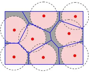
In a Voronoi diagram, all the points within a Voronoi cell are closest to the generating node that lies within that cell. Thus, having constructed the Voronoi diagram of the sensor nodes and overlaid the sensing regions on it (Figure 2), if a point of a Voronoi cell is not covered by its generating node, this point is not covered by any other sensors (Ahmed et al., 2005 ; Ghosh, 2004; Wang et al., 2009; Wang et al., 2003) and results in coverage holes in the region of interest. If the sensors have the ability to move in the network, their movement may fill the
coverage holes. Three movement strategies based on Voronoi diagram have been proposed by Wang et al. (2006), which are Vector-Based (VEC), MiniMax, and Voronoi-Based (VOR) algorithms, all of which improve the sensors network coverage in an iterative manner. In the following, the VOR algorithm is described, and will be improved and extended to 3D environments in the next section.
Figure 2. Coverage hole (gray regions) in a WSN overlaid on the Voronoi diagram of the sensors
The VOR is a pulling strategy so that sensors cover their local maximum coverage holes. In this algorithm, each sensor moves toward its furthest Voronoi vertex till this vertex is covered (Figure 3).
Initial Round 1
Round 2 Round 3
Round 4 Round 5
Figure 4. An example of sensor deployment based on the VOR algorithm (Wang et al., 2006)
4. EXTENDING THE VOR ALGORITHM TO 3D ENVIRONMENTS
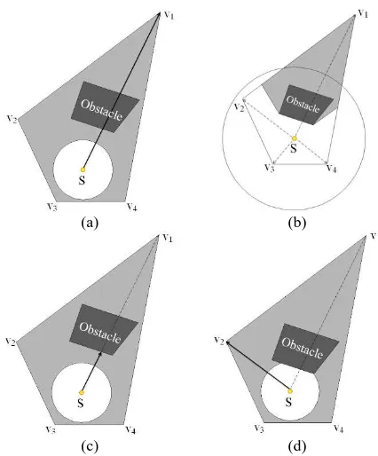
The VOR algorithm is capable of equally distributing the sensors in the region. However, it has been developed for plain 2D spaces and does not consider any constraint forced by the environment. We improve the VOR algorithm so that it can be applied to geosensors in 3D environments and supports visibility, obstacles and forbidden regions (i.e., the regions in which none of sensor are allowed to be placed). This is done through considering the above constraints in the sensor movements. In the proposed algorithm, only those sensors whose furthest vertex is not covered will move: If all visible Voronoi vertices are covered by the sensor (Figure 5.b), that sensor will not move. Otherwise, the sensor moves toward the furthest vertex. In case this furthest vertex is hidden by an obstacle (which is determined through 3D visibility analysis), the movement length is calculated with respect to the distance between the sensor and the obstacle (Figure 5.c). If no movement is possible toward the furthest vertex due to the obstacles, the second furthest vertex is chosen (Figure 5.d), which automatically provides supporting forbidden regions (i.e., avoiding the sensor to move into the forbidden regions).
(a) (b)
(c) (d)
Figure 5. Simple and extended VOR algorithms: (a) simple VOR, in which the sensor moves without considering the obstacle; (b) If all Voronoi vertices (except v1) correspond to the sensor are covered, that sensor will not move; (c) Movement of the sensor toward the furthest vertex with respect to the distance between the sensor and the obstacle; (d) Movement toward the second furthest vertex, if no movement is possible toward the furthest vertex due to obstacles
Another improvement was also applied on the simple VOR algorithm, which is about the movement length: In the simple VOR, the sensor always moves until covers the furthest Voronoi vertex or at least its new position provides more coverage of the Voronoi cell than the current position. This strategy may results in a new hole on another vertex. Our solution is that the next movements should not change the geometry of the Voronoi cell too much. To take these consideration into account, our algorithm applies a shorter movement at each next step.
5. IMPLEMENTATION RESULTS
Figure 6. The sample 3D raster environment
In order to evaluate the stability of the proposed approach, both algorithms (simple and extended VOR algorithm) were run for 50 times and some parameter such as average, variance, maximum and minimum of the covered area percentage were calculated (Table 1), which certifies providing better results by the proposed method. Furthermore, Figure 8 shows the position of the sensors for both cases in different steps. The simple VOR algorithm does not consider the obstacles and just distributes the sensors in an equivalent configuration (Figure 8.a), while no sensor is deployed in the forbidden areas in the proposed method (Figure 8.b).
Initial Round 1
Round 2 Round 3
Figure 7. The results of applying the extended proposed VOR algorithm on a set of sample sensors
(a)
(b)
Figure 8. Position of the sensors for both cases in different steps (a) simple VOR algorithm; (b) extended VOR algorithm
Algorithm Simple VOR Extended VOR
Coverage %
Average 56.4122 75.4123
Variance 11.2996 1.53410
STD 3.36148 1.2385
Max 59.1811 77.7044
Min 39.9006 72.1707
Table 1. Comparison of simple and extended VOR algorithm
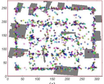
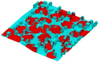
As a second example, a 3D terrain topography consists of numerous buildings and some trees as obstacles was considered (Figure 9) and the extended VOR algorithm was applied on an initial configuration of a set of sensors distributed in the environment (Figure 10). The result of the sensor deployment after 50 iterations is illustrated in Figure 11.
Figure 9. The 3D terrain topography and features
Figure 11. Coverage of the sensors (red regions) for Position of the sensors after 50 iterations of the extended VOR algorithm
6. CONCLUSIONS AND FUTURE WORK
This paper proposed an extension to a Voronoi-based deployment algorithm in order to be applied on 3D environments, which takes the 3D features into account. In this case, the visibility and viewshed analyses are used to estimate the sensor coverage, which means that a real 3D model is considered. The results of the proposed extended method applied on two case studies certify the improvement achieved. The environments used in both of the case studies were 3D raster. We expect that the spatial resolution of the raster model will influence the sensor deployment, which will be evaluated in the future. Furthermore as we are working, in parallel, on sensor coverage estimation in 3D vector environments, the proposed deployment optimization method will be applied on 3D vector models in order to evaluate the effect of quality of the models on the final sensor deployment and coverage estimation. Finally, extending other Voronoi-based sensor deployment methods will be considered as a future direction.
7. ACKNOWLEDGMENT
The authors would like to deeply appreciate Filip Biljecki for providing the CityGML data, without which the implementations and comparisons could not have been performed.
REFERENCES
Ahmed, N., Kanhere, S.S., Jha, S., 2005 The holes problem in wireless sensor networks: a survey. ACM SIGMOBILE Mobile Computing and Communications Review 9, 4 - 18.
Akbarzadeh, V., Hung- Ren Ko, A., Gagn'e, C., Parizeau, M., 2010. Topography-Aware Sensor Deployment Optimization with CMA-ES, Parallel Problem Solving from Nature, PPSN XI. Springer, pp. 141-150.
Argany, M., Mostafavi, M.A., Karimipour, F., 2010. Voronoi-based Approaches for Geosensor Networks Coverage Determination and Optimisation: A Survey, Proceedings of the 7th International Symposium on Voronoi Diagrams in Science and Engineering (ISVD 2010), Quebec, Canada, pp. 115-123.
Argany, M., Mostafavi, M.A., Karimipour, F., Gagné, C., 2011. A gis based wireless sensor network coverage estimation and optimization: A voronoi ap-proach. Transacton on Computational Sciences Journal 14, 151-172.
Chong, C.Y., Kumar, S.P., 2003. Sensor networks: evolution, opportunities, and challenges. Proceedings of the IEEE 91, 1247 - 1256.
Ghosh, A., 2004. Estimating Coverage Holes and Enhancing Coverage in Mixed Sensor Networks, Local Computer Networks, 2004. 29th Annual IEEE International Conference on, pp. 68 - 76.
Ghosh, A., Das, S.K., 2006. Coverage and connectivity issues in wireless sensor networks. Mobile, Wireless, and Sensor Networks: Technology, Applications, and Future Directions, 221-256.
Hossain, A., Biswas, P.K., Chakrabarti, S., 2008. Sensing Models and Its Impact on Network Coverage in Wireless Sensor Network, Industrial and Information Systems, 2008. ICIIS 2008. IEEE Region 10 and the Third international Conference on. IEEE, Kharagpur, pp. 1 - 5.
Howard, A., Matari´, M.J., Sukhatme, G.S., 2002. Mobile Sensor Network Deployment using Potential Fields, A Distributed, Scalable Solution to the Area Coverage Problem, 6th International Symposium on Distributed Autonomous
Robotic Systems (DARS‘02), Fukuoka, Japan.
Howard, A., Matari´, M.J., Sukhatme, G.S., 2002 An Incremental Self-Deployment Algorithm for Mobile Sensor Networks. Autonomous Robots 13, 113-126
Karimipour, F., Argany, M., Mostafavi, M.A., 2013. Spatial coverage estimation and optimization in geosensor networks deployment, Wireless sensor networks: From theory to applications. CRC Press.
Ma, H., Zhang, X., Ming, A., 2009. A Coverage-Enhancing Method for 3D Directional Sensor Networks, INFOCOM 2009, IEEE. IEEE, Rio de Janeiro, pp. 2791 - 2795.
Megerian, S., Koushanfar, F., Potkonjak, M., Srivastava, M.B., 2005 Worst and Best-Case Coverage in Sensor Networks. IEEE Transactions on Mobile Computing 4, 84-92
Nittel, S., 2009. A Survey of Geosensor Networks: Advances in Dynamic Environmental Monitoring. Sensors 8, 5664–5678.
Szewczyk, R., Osterweil, E., Polastre, J., Hamilton, M., Mainwaring, A., Estrin, D., 2004. Habitat monitoring with sensor networks. Communications of the ACM 47, 34-40.
Wang, B., Lim, H.B., Ma, D., 2009. A survey of movement strategies for improving network coverage in wireless sensor networks. Computer Communications 32, 1427–1436.
Wang, G., Cao, G., La Porta, T., 2006. Movement-Assisted Sensor Deployment. Mobile Computing, IEEE Transactions 5, 640 - 652.
Wang, G., Cao, G., LaPorta, T., 2003. A Bidding Protocol for Deploying Mobile Sensors, ICNP '03 Proceedings of the 11th IEEE International Conference on Network Protocols.
Wang, Y., Cao, G., 2011. Barrier Coverage in Camera Sensor Networks. MobiHoc '11 Proceedings of the Twelfth ACM International Symposium on Mobile Ad Hoc Networking and Computing.
Worboys, M., Duckham, M., 2006. Monitoring qualitative spatiotemporal change for geosensor networks. International Journal of Geographical Information Science, 1087-1108.
Zou, Y., Chakrabarty, K., 2003. Sensor Deployment and Target Localization Based on Virtual Forces, INFOCOM 2003. Twenty-Second Annual Joint Conference of the IEEE Computer and Communications. IEEE Societies. IEEE, San Francisco, CA, pp. 1293 - 1303.