GPS-DENIED GEO-LOCALISATION USING VISUAL ODOMETRY
Ashish Gupta∗, Huan Chang, Alper Yilmaz
The Ohio State University, Columbus, Ohio, United States - (gupta.637, chang.1522, yilmaz.15)@osu.edu
Commission III, WG III/3
KEY WORDS:GPS-denied, Geo-localisation, 3D view geometry, computer vision,GIS,OpenStreetMap
ABSTRACT:
The primary method for geo-localization is based on GPS which has issues of localization accuracy, power consumption, and unavail-ability. This paper proposes a novel approach to geo-localization in a GPS-denied environment for a mobile platform. Our approach has two principal components: public domain transport network data available in GIS databases or OpenStreetMap; and a trajectory of a mobile platform. This trajectory is estimated using visual odometry and 3D view geometry. The transport map information is abstracted as a graph data structure, where various types of roads are modelled as graph edges and typically intersections are modelled as graph nodes. A search for the trajectory in real time in the graph yields the geo-location of the mobile platform. Our approach uses a simple visual sensor and it has a low memory and computational footprint. In this paper, we demonstrate our method for trajectory estimation and provide examples of geolocalization using public-domain map data. With the rapid proliferation of visual sensors as part of automated driving technology and continuous growth in public domain map data, our approach has the potential to completely augment, or even supplant, GPS based navigation since it functions in all environments.
1. INTRODUCTION
Autonomous navigation is an emerging technology with a huge potential; self-driving cars are almost round the corner. This tech-nology requires accurate geo-localization in real-time to effec-tively navigate urban environments. Currently, navigation tech-nologies are GPS reliant, which has multiple issues. The accu-racy of standard GPS devices is unacceptably poor for the pur-poses of autonomous navigation and accurate GPS sensors are very expensive. GPS is unreliable in several environments where transmission between the device and satellites is impeded by sur-rounding structures, like tall buildings in an urban environment, the so called ’urban canyons’. In addition, GPS is unavailable in-doors, underground, in tunnels, etc. and can also be degraded or denied in certain geographic regions. In order to be viable for a huge consumer market, there is a need for geo-localization solu-tion that operates with low-cost sensors and public domain data.
The DARPA grand challenge has demonstrated the effectiveness of visual sensors in autonomous navigation by analyzing visual information for video cameras mounted on the mobile platform. There are arguably two main conceptual approaches for vision based methods. One of these approaches seeks to use an ever growing geo-tagged image database, as in Google Street View. The images from the camera are queried to this database and matches are used to infer the geo-location of the mobile platform in real-time (Vaca-Castano et al., 2012). While such localiza-tion results show promise, this approach requires a maintenance and continuous access to very large image databases which is ex-tremely expensive and not currently not a feasible solution (Paul and Newman, 2010). The second approach is inspired by naviga-tion in robotics using SLAM, which perform a localizanaviga-tion and mapping of the neighborhood of the robot. The key issue with SLAM framework is the accumulation of drift error that results in poor localization, which is more pronounced for traversals over long distances .
This paper poses the problem of accurate geo-localization as a combination of accurate relative localization within a very large
∗Corresponding author
spatial search space. The relative localization is computed using Visual Odometry (VO) and the large spatial search space is ac-quired from GIS databases. The key insight in this paper is that the motion of the typical mobile platform is correlated to the as-sociated topology of the spatial search space. For example, a car moves on roads and so the trajectory of the car for a finite dis-tance of travel is correlated to a subset of the transport network layer of GIS in the spatial search space for that car. The use of one or more layers of GIS based on the type of mobile platform and sensors facilitates flexibility in our approach and the ability to scale the solution.
The combination of Inertial Measurement Units (IMUs) and vi-sual sensors is a crucial and useful technique for autonomous nav-igation, particularly in unknown indoor or GPS-denied environ-ments. Although pure monocular vision-based Extended Kalman Filter (EKF) can achieve around meter level of the trajectory er-ror, it is limited in a small or well constraint area in order to avoid scale drift (Civera et al., 2010). Using sequential stereo pairs or camera matrix is capable of handling the scaling problem as a depth measurement based on epipolar geometry, with well-calibrated camera interior orientation parameters (IOP) and rela-tive exterior orientation parameters (EOP). However, the shutter synchronization, calibration bias and other uncertainties between camera pairs will lead to a camera trajectory drift. A robust on-site calibration with the unknown features in the scenes is still an unsolved problem. In this perspective, using monocular cam-era visual odometry is more practicable than stereo pairs or other depth measurement device.
noise and bias inherent in these measurements are multiplied and cumulative after each integration, causes the system pose drift to become significantly unbounded over time. To overcome these drawbacks of the IMU drifting problem, the camera is capable of detecting feature points in the scenes and using them as a pose constraint. In synergy, IMU provides short-term reliable system pose for camera to measure unknown features in the scenes as 3D landmarks.
Our contributions in this paper are: (i) we introduce a novel ap-proach to geo-localization of mobile platforms in real-time that combines GIS/OpenStreetMap data and visual sensors on-board the mobile platform. We demonstrate a computationally efficient approach at is scalable to search accurate geo-location in a very large region of interest; and (ii) this study proposed a visual-inertial navigation system (VINS), including monocular visual odometry and IMU. Proposed method improved feature track-ing and camera measurement results, providtrack-ing better EKF-based visual-inertial pose estimation.
2. RELATED WORK
Global localization is an important part of any autonomous nav-igation system and its uninterrupted performance is crucial for the stability and robustness of the system. To achieve this goal, several visual odometry based approaches have emerged in re-cent years, offering high quality localization performance even at real-time execution speeds. The basic pipeline of these methods includes a feature extraction stage, followed by feature match-ing, 3D reconstruction of a sparse point cloud, and finally esti-mation of the pose of the mobile platform. A windowed bundle adjustment is typically run at the end. The main drawback of this category of methods is that drift is accumulated over time. As a result, after the mobile platform has travelled a certain distance, the localization error becomes significant, making the localiza-tion result unusable over longer distances (Engel et al., 2015). In parallel to the VO approaches, there are a number of methods that perform visual-SLAM (Lategahn et al., 2011). The vSLAM ap-proach is similar to VO, differing in that reconstructed 3D points are used as landmarks and their position is optimized together with the camera pose.
There has been research towards using map information that is already available in the form of 2D (e.g., Google Maps, Open-StreetMaps) or 3D road maps (e.g., Google Maps 3D) for local-ization. (Hentschel and Wagner, 2010) propose the use of Open-StreetMap maps to facilitate robot localization and navigation. A cadastral map with the building footprints is extracted and the GPS position of the robot is used in an MCL framework to pro-vide localization for the robot. Recently, (Senlet and Elgammal, 2011) have presented a system that uses Google Static Maps to perform global localization. In particular, they perform a local reconstruction of the scene, using stereo depth maps, which they later compare with the 2D map. Both of the aforementioned ap-proaches show the potential that the use of map information can bring to the localization task. However, these systems require a manual initial localization and have only been tested in suburban areas where the environment is relatively simple and the paths they have travelled are short in length.
Elaborating on VO methods, a majority focus on integrating IMU and monocular vision using filter-based(KF, Information Filter, particle filter), EM-based, or batch optimization (shape from mo-tion) (Strelow and Singh, 2004) methods. Bundle adjustment is a non-linear global optimization approach, which can produces estimates of the sensor motion, 3D points structure of the scenes, and other unknown variables (e.g.. biases) using measurements
from the entire observation simultaneously. But the computation cost and complexity is to heavy, especially when the image se-quence is long.
EM iterates two major steps, expectation step for posterior sys-tem pose from map; and maximization step to find most likely pose from the expectations, and finally build up a series of in-creasingly accurate maps. EKF-based SLAM is another efficient recursive algorithm. EKF-based approach provides optimal min-imum mean-square Error (MMSE) estimates of the state (device and landmark positions), and its covariance matrix seems to con-verge strongly. However, the Gaussian noise assumption restricts the adaptability of the EM and KF for data association and num-ber of landmarks. Sliding Window Filter (SWF) is a keyframe-based operating method, performing a batch optimization over a set number of system states, which is useful for large scale opera-tions. Multi-State Constraint Kalman Filter (MSCKF) (Mourikis and Roumeliotis, 2007) preserve a buffer window of sensor poses and simultaneously update each pose in the window using batch-optimized estimates of observed landmarks across the buffer win-dow. This study implement MSCKF for Camera-IMU trajectory estimation, and improved a more robust landmark feature de-scriptor for tracking process. Camera-IMU calibration and data synchronization are the priori Information for the developed VINS. These calibration parameters are including time scaling and off-set, relative pose between IMU and camera, and IMU bias. (Ovr´en and Forss´en, 2015) proposed a non-linear least squares minimiza-tion method using the symmetric transfer error as cost funcminimiza-tion, joint calibration of a wide-angle rolling shutter camera and an ex-ternally mounted gyroscope. Calibration of camera IOP includes principle points, focal length and lens distortion. Observed im-ages then can correct deformation regarding IOP for higher ac-curacy matching process. Domain-size pooling scale-invariant feature transform (DSP-SIFT) (Dong and Soatto, 2015) improve the robustness of point-based descriptor by pooling gradient ori-entations across different domain sizes. This kept the dimension remains the same but more appropriate for against photometric nuisances.
3. METHODOLOGY
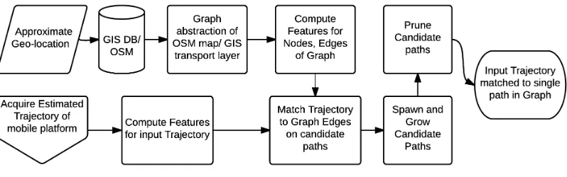
We pose the problem of accurate mobile platform geo-localization as a combination of approximate geo-localization and accurate relative localization. The approach requires an initial hypothesis of region where the mobile platform can be located, which can be arbitrarily large from size of a village to the entire globe, though computational complexity scales with a larger search space. For typical use cases, the region of interest would be a political state or city sized area, which we have selected for our experiments in this paper. Our approach is illustrated in the block diagram in Figure 1.
The first step is to acquire map data from a public domain source like OpenStreetMap (OSM) or Geographic Information System (GIS) databases. OpenStreetMap data can be accessed via the corresponding website, and the user can download the map for the region of interest by specifying a bounding boxbin terms of longitude and latitude, b =(latmin, lonmin, latmax, lonmax).
The map is given in XML format and is structured using three basic entities: nodes, ways and relations. The nodenrepresents a point element in the map and is defined by its GPS coordinates, longitude and latituden= (lat, lon). Linear and area elements are represented by waysw, which are formed as a collection of nodes
w = {ni}i=1...k. The relationsrare used to represent
Figure 1: Mobile Trajectory Geo-Localization: VO is used to compute a trajectory in real-time which is abstracted as a sub-graph and is progressively localized by sub-graph matching in a graph abstraction of transport network map of the region of interest.
us are streets, which are modelled as ways, and can be extracted from the XML data in to form a street graph of the region of in-terest. Map data can also be acquired from GIS databases in the form of ’shapefiles’ format, that is a popular geospatial vector data format developed and regulated by Esri. Similar to OSM, the shapefile data is used to construct a road network graph. A example of OpenStreetMap, shapefile and computed transport network graph is shown in Figure 2. Community contributed data sources like OpenStreetMap are being continuously updated whereas shapefile databases are comparatively better curated and updated more infrequently. The choice of data source would de-pend on the region of interest and the current state of respective maps of that region. In addition, it should be noted that conve-nience of data access comes with the cost of registration errors and noise which makes the task of searching the mobile plat-form trajectory in the graph more difficult. The second step is to compute feature descriptors for the 3D trajectory of the mobile platform and the transport network graph. We chose a contour tangent angleθ as uniform sample distance, illustrated in Fig-ure 4a for the featFig-ure descriptor as a trade-off between demands for computational efficiency in processing and storage, robust-ness to noise and missing data, and scalability. There exist sim-ple to comsim-plex trajectory descriptors with inbuilt invariance and other features, but have a corresponding high computational and storage cost. In order to aid scalability of the solution and sim-ple enough so it can be deployed on mobile computational plat-forms with comparatively low processing power, we opted for a descriptor that is both fast and good for search trajectory in the graph. A trajectoryT ={P1, P2, . . . , Pn}consists of points at
roughly uniform sampling distance. The quantization associated with sampling distance is relevant in terms of sensitivity to the motion of the mobile platform (for example, swerve, lane-change and over-taking motion of a car) and also relevant to scalabil-ity. Our choice of sampling distance was empirically determined. The motion from pointPtto pointPt+1is encoded in terms of
the angleθ, shown in Figure 3a, and its associated bin. We found quantizing the contour angles to72bins,θ∈[0, . . . ,71], worked well in our experiments. The choice of quantization level is based on optimizing sensitivity to mobile platform motion while mini-mizing effect of noise. Figure 4b shows a trajectory encoded in this manner.
3.1 Trajectory Search in Graph
To find the mobile platform trajectory in the road network, we ab-stract both to a graph data structure and pose the problem of tra-jectory search as a sub-graph matching problem, where the graph of the trajectory of a mobile platform travelling on the roads of
a map is a sub-graph of the entire map graph. The transport net-work mapMhas been abstracted as a graphGM, illustrated in Figure 2c. The trajectoryτis abstracted as a graphGτ. Graph
matching works by computing equivalent features on both map graphGMand trajectory graphGτand storing these feature
val-ues at the nodes and or edges of the graph, which are then used to compute a similarity score between trajectory graph and a path graphGP, which is a hypothesis of a matching sub-graph ofGM.
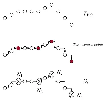
With the aim of facilitating a generalized solution that does not require knowledge of geographic coordinates or global direction information of the mobile platform, we assume that the trajectory estimated by VO is in its simplistic form a sequence of points with relative distance measure. This means the most reliable mode of encoding the trajectory is change in angle of motion of the mo-bile platform which is equivalent to contour angles of a spline approximation of the acquired sequence of points. Figure 5 il-lustrates an acquired trajectory as a set of pointsTV O. We
com-pute a spline approximation using these points and those points with significant change in contour angle are selected as ’control points’. A graph abstraction of this trajectoryGτis created using
the control points as nodes of the graph and set of points between control points comprise an edge of the graph, wherein are com-putingTV O→ Gτ. Since the mobile platform travels on the road
network the trajectory graph can be assumed to be a sub-graph of the map graph,Gτ⊂ GM. Our approach to searching for a match
inGMis to introduce ’path graph’GP. Searching forGτ⊂ GM
is equivalent to search for a sub-graphGP ofGMsuch that the trajectory is similar to this path sub-graphGτ ≡ GP. So, we
compute a similarity scoreS(·,·)between the trajectory graph and path graph,S(Gτ,GP)∀ GP ⊂ GM, for all path graphs in
the map graph. The best matching path graph is
GP∗ ←arg max GP
S(Gτ,GP)∀ GP ⊂ GM
We are considering the problem of geo-localization in real-time. The estimated trajectoryTV Ocontinuously grows with time and
consequently the trajectory graph also grows with time. Conse-quently we formulate our trajectory search solution accordingly, where best matching solution at timetis given in equation 1.
GP(t)∗←arg max GP(t)
S(G(t)
τ ,G
(t)
P )∀ G
(t)
P ⊂ GM (1)
In our implementationS(·,·)is computed using a sub-string match-ing algorithm. The trajectory Gτ(t) is a sequence of quantized
(a) OpenStreetMap (b) GIS ShapeFile (c) Graph representation
Figure 2: Abstraction of OpenStreetMap or GIS data to a transport network Graph representation
(a) Encoding trajectory of mobile platform and edges on graph of transport net-work. The motion from point
Pt at sampling interval tto
Pt+1is measured in angleθ
which is quantized to corre-sponding bin. (This illustra-tion uses 8 bins for visual-ization, though in our imple-mentation we use 72 bins.)
(b) Features for undirected graph are computed as angles between each pair of edges at each nodeN0with its
neigh-bors N = {N1, N2, N3}. The features[θ0210, θ2003, θ0130]is
stored at each node of the graphGM
.
Figure 3: Encoding mobile platform trajectory and graph.
(a) 3D trajectory descriptor (b) Road graph descriptor
Figure 4: Feature descriptor for estimated 3D trajectory of mobile platform and edges of graph representing roads. The descriptor is computationally efficient and facilitates matching between the trajectory of the mobile platform and the transport network graph.
The key benefit of using string matching is that partial matches also produce a reasonably good similarity score. This formulation makesS(·,·)robust to noise, missing data, erroneous vehicle mo-tion like swerving, map registramo-tion flaws, etc. The motivamo-tion for this approach is derived from the popular Bag-of-Words method
Figure 5: The trajectory estimated from visual odometryTV Ois
a sequence of points with relative vector information. A subset of these points where there is significant change in contour are selected a ’control points’, which become nodes in a trajectory graphGτ
in computer vision that has also been used for SLAM (Paul and Newman, 2010).
3.2 Visual Odometry
Figure 6: Visual Odometry
3.2.1 Feature detection and tracking Feature extraction and tracking is the essential work for vision-based mapping and tra-jectory estimation. Scale-invariant feature transform (SIFT) is a well-known feature point descriptor, which was designed to re-duce variability due to illumination while retaining discriminative power in the scale space. Each un-normalized cell of SIFT can be written as:
hS(θ, I, σ)(x) =
Z
Eǫ(∠∇I(y)−θ)Eσ(y−x)k ∇I(y)kdy,
whereI is the image window of the centred pixelxwith spa-tial pooling scaleσ. θis corresponding to orientation histogram bin (ǫ), normally with 8 direction from 0 to2π. KernelEǫand
Esigmarepresents a bilinear of sizeǫand separable-bilinear of
sizeσ, respectively. The SIFT descriptor is a 128-dimensional vector that is a concatenation of a normalized4×4cells with 8 bins. DSP-SIFT is a modified form of the standard SIFT, ob-tained by pooling gradient orientations from different scaled do-main sizes, instead of spatial space. The formula is given by:
hDSP(θ, I)(x) =
Z
hS(θ, I, σ)(x)ǫs(σ)dσ, (2)
whereE is an exponential unilateral density function ands is the size-pooling scale. DSP-SIFT kept the same descriptor di-mension but more suitable for searching correspondence in the presence of occlusions.
After extracting feature points and their DSP-SIFT descriptors between subsequent images, a perspective homography constrain was applied to filter outliers by mapping one image to another. ’Inliers’ are considered if the co-planar feature points between subsequent images are fully matched or within a small displace-ment. The Random sample consensus (RANSAC) algorithm was applied to optimize the homography transformation under the over-constrained degree of freedom problem. RANSAC uses iter-ative calculations to estimate optimal parameters of homography matrix (8 DOF) from observations, and removed outliers from the matching process.
3.2.2 Visual-inertial trajectory estimation We implemented a multi-state constraint Kalman filter to combine the IMU and
monocular vision-based measurements. Tracked pose of the Camera-IMU sensor are presented based on the Centered, Earth-Fixed (ECEF) coordinates. Initial camera poses were given by the EKF propagating state and covariance, updated from multi-observed feature points, assuming that N camera poses are in-cluded in the EKF state at each time stepk. The state and error-state vector are:
whereqIG,kis the unit quaternion representing the rotation from
global frame Gto the IMU frame I at time k. pIG,k is the
IMU position with respect to global frame.bgandbaare the
bi-ases of gyroscope and accelerometer measurements, respectively.
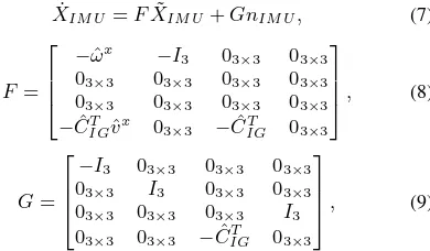
δΘdescribed the attitude errors is a minimal representation. To sum up, at timek, the full state of the KF consists of the 13-dimensional IMU state andN×7-dimensional past camera poses in which active feature tracks were visible. In the propagation step, the filter propagation equations are derived by discretiza-tion of the continuous-time IMU system model, the linearized continuous-time model is formulated:
wherenIM Uis the system noise. The covariance matrix ofnIM U
is computed off-line during sensor calibration. The matricesF
andGare the Jacobians;I3is3×3identity matrix;ωandvare
3×3rotational velocity and linear velocity matrix, respectively;
CIGT is the rotation matrix corresponding toq T
IG.
Every IMU readings are used for the state propagation in the EKF. Moreover, the EKF covariance matrix has to be propagated every k+1 steps. State covariance is a(12 + 6N)×(12 + 6N)matrix and state covariance propagation is given by:
Pk|k=
12×12covariance matrix of the current IMU state;PCC is the
6N×6Ncovariance matrix of the camera poses; andPICis the
12×6Ncorrelation between the errors in the IMU state and the camera pose estimates.
When capturing a new video frame, the camera pose estimation is computed from the IMU pose estimation. This camera pose estimate is appended to the state vector, and the covariance matrix of the EKF is augmented as:
0 50 100 150 200 250 300 350 400
(b) 3D trajectory (c) 3D point cloud
Figure 7: The trajectory estimated by our method from 3D point cloud
Jk=
whereJk is the Jacobian matrix,fj is a feature point that has
been observed from a set ofMjcamera poses. We use an
in-verse depth least-squares Gauss-Newton optimization method to estimate three-dimensional location offj. The residual for each
measurement is independent of the errors in the feature coordi-nates, and thus EKF updates can be performed based on it.HXi andHfi are the Jacobians of the measurementzi with respect to the state and the feature position, respectively. Kalman gain can then be calculated asK = P THT(THP THT +Rn)(−1),
whereTHis an upper triangular matrix from QR decomposition
of the matrixHX. Finally, the state covariance matrix is updated
according to
Pk+1|k= (Iξ−KTH)Pk+1|k(Iξ−KTH)T+KRnKT. (13)
4. EXPERIMENTS
In our experiments we evaluate our visual odometry pipeline in 4.1 and demonstrate our geo-localization approach in 4.2 using maps acquired fromOpenStreetMapand GIS from different urban and semi-urban regions in different parts of the world.
4.1 Visual Odometry
The IMU data provided in this dataset was recorded byOXTS RT 3003, containing acceleration and angular rate around three axes with 100 Hz sampling rate. Video frames were captured us-ing Point Grey Flea 2 (FL2-14S3M-C) in gray-scale with 1242 ×375 pixels resolution (after calibration). Shutter time adjusted dynamically (maximum shutter time: 2 ms) and triggered at 10 Hz frequencies. This dataset provides well-calibrated camera in-trinsic parameters and camera-IMU rotation and translation ma-trix. The synchronized IMU and video frames are at 10Hz for this study.
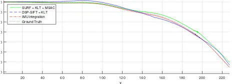
Figure 7 demonstrated the trajectory estimated for a long term tracking case. The translational average root mean squared error (ARMSE) is4.154m, rotational ARMSE is0.026m, and final translational error is12.149m. The accuracy for the estimated is capable for proposed GIS path searching algorithm. Figure 8 demonstrated the comparison between proposed method, IMU in-tegration and MSCKF implemented by (Clement et al., 2015) on case no. 0051. Table 1 quantified the error ARMSE with two other visual-initial approaches, MSCKF and SWF.
4.2 Geo-localization
We found that abstraction of trajectory and map to graph struc-ture should we based on the scale and frequency of occurrence of significant features. To improve efficiency of the implementation
Dataset ID 0001 0005 0035 0051 0095 IMU Tra. ARMSE 0.784 0.965 0.263 2.255 1.945
Rot. ARMSE 0.003 0.015 0.009 0.008 0.007 Final Tra. Err. 2.532 3.109 0.469 6.335 7.592 MSCKF Tra. ARMSE 0.449 1.217 0.268 2.310 1.324 Rot. ARMSE 0.007 0.023 0.009 0.028 0.046 Final Tra. Err. 1.130 2.453 1.879 9.294 3.628 SWF Tra. ARMSE 0.432 0.968 0.279 1.178 1.900 Rot. ARMSE 0.007 0.023 0.006 0.016 0.010 Final Tra. Err. 1.136 3.712 0.719 2.167 7.579 Our Tra. ARMSE 0.342 1.115 0.269 2.875 1.885 Rot. ARMSE 0.009 0.011 0.011 0.032 0.146 Final Tra. Err. 1.797 3.053 1.577 4.742 5.738
Table 1: Comparison of translation ARMSE, rotation ARMSE, and final translation error of proposed method, MSCKF, and SWF on KITTI dataset. (units:m)
20 40 60 80 100 120 140 160 180 200 220
Figure 8: The comparison between proposed method, IMU inte-gration and MSCKF on case no.0051.
we begin with an analysis of the topology of map data acquired fromOpenStreetMap, described in 4.2.1. There results were used to tune the parameters of our geo-localization pipeline which is evaluated on several instances of regions from different parts of the world in 4.2.2.
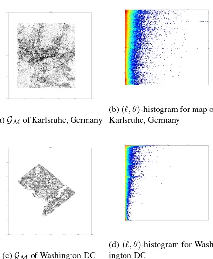
4.2.1 Map Features The number and location of nodes and edges ofGMabstracted from theOSMmap should be based on the degree of quantization that reduces the computational com-plexity while preserving the uniqueness of different edges and subsequently path graphsGPso that the search and converge to the best matchingG∗
(a)GMof Karlsruhe, Germany
(b)(ℓ, θ)-histogram for map of Karlsruhe, Germany
(c)GMof Washington DC
(d)(ℓ, θ)-histogram for Wash-ington DC
Figure 9: Analysis of GM of urban and semi-urban cities of Washington DC and Karlsruhe, Germany. The graphs shows the (ℓ, θ)-histogram of the lengthℓand orientationsθof the edges of GM(columns correspond to edge lengthsℓand rows correspond to edge orientationsθ). The lattice structured urban and spaghetti structured semi-urban graphs show different histograms reflect-ing the inherent difference in these two types of maps.
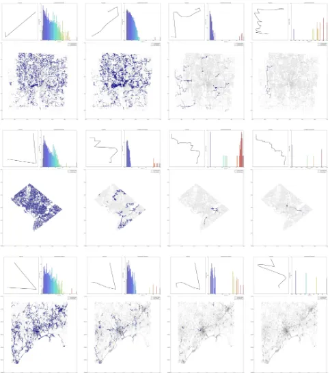
4.2.2 Trajectory search We acquired maps for regions of in-terest from OpenStreetMap and GIS database to evaluate the per-formance of our approach for different types of transport net-work topologies including urban, semi-urban and country roads, and scale of the search region. We selected maps for: ’Franklin county, Ohio’ which provides a typical U.S. county sized map; ’Washington DC’, which is a highly urban region with a lattice grid structured road network; and ’Montpellier, France’, which is a semi-urban and country spaghetti shaped road network of a state sized region. Some of the results of our experiments for each of these regions is illustrated in Figure 10. Initially, the esti-mated trajectoryGt0
τ is short as the mobile platform begins
mov-ing. We computeGPand associated similarity scoreS(Gτt0,GP)
and there are several matching paths, shown in the first column of the figure for each region. As the estimated trajectory growsGtn
τ
the number of candidate paths reduce based on our empirically determined threshold, shown in the center column in the figure. Subsequently, a single path with the highest similarity score re-mains, which is our matched path in the map graph. The right column for each region in the figure shows the matched path in the graph for the corresponding mobile platform trajectory. In our experiments we found that quick search depends on the unique-ness of the trajectory and the nature of the map graph.
5. CONCLUSION
We have presented a novel approach for geo-localizing position of a mobile platform. We have proposed a modified approach to classical visual odometry pipeline with map data from public do-main sources likeOpenStreetMapsandGIS databasesin a unified
framework. We have described the algorithmic and implementa-tion details of our method and demonstrated it on several differ-ent types of maps from differdiffer-ent regions of the world. We have demonstrated excellent results on our proposed visual odometry pipeline on benchmark KITTI dataset. Our results show that the proposed system is able to provide fully automatic global local-ization at a low infrastructural cost. Building on this work, we plan to further investigate the use of maps, especially different layers of a GIS database such as building, hydrology, relief maps, etc. We also plan to integrate outdoor and indoor GPS-denied navigation for seamless uninterrupted geo-navigation in all loca-tions and environment condiloca-tions.
REFERENCES
Civera, J., Grasa, O. G., Davison, A. J. and Montiel, J. M. M., 2010. 1point ransac for extended kalman filtering: Application to realtime structure from motion and visual odometry. Journal of Field Robotics 27(5), pp. 609–631.
Clement, L. E., Peretroukhin, V., Lambert, J. and Kelly, J., 2015. The battle for filter supremacy: A comparative study of the multi-state constraint kalman filter and the sliding window filter. In: Computer and Robot Vision (CRV), 2015 12th Conference on.
Dong, J. and Soatto, S., 2015. Domain-size pooling in local de-scriptors: Dsp-sift. In: Computer Vision and Pattern Recognition (CVPR), 2015 IEEE Conference on, pp. 5097–5106.
Engel, J., St¨uckler, J. and Cremers, D., 2015. Large-scale direct slam with stereo cameras. In: IEEE/RSJ International Confer-ence on Intelligent Robots and Systems.
Hentschel, M. and Wagner, B., 2010. Autonomous robot navi-gation based on OpenStreetMap geodata. Intelligent Transporta-tion Systems (ITSC), 2010 13th InternaTransporta-tional IEEE Conference on pp. 1645–1650.
Lategahn, H., Geiger, A. and Kitt, B., 2011. Visual SLAM for autonomous ground vehicles. Proceedings - IEEE International Conference on Robotics and Automation pp. 1732–1737.
Mourikis, A. and Roumeliotis, S., 2007. A multi-state constraint kalman filter for vision-aided inertial navigation. In: Robotics and Automation (ICRA), 2007 IEEE International Conference on, IEEE, pp. 3565–3572.
Ovr´en, H. and Forss´en, P.-E., 2015. Gyroscope-based video stabilisation with auto-calibration. In: Robotics and Automa-tion (ICRA), 2015 IEEE InternaAutoma-tional Conference on, IEEE, pp. 2090–2097.
Paul, R. and Newman, P., 2010. FAB-MAP 3D: Topological map-ping with spatial and visual appearance. Proceedings - IEEE In-ternational Conference on Robotics and Automation pp. 2649– 2656.
Senlet, T. and Elgammal, A., 2011. A framework for global vehicle localization using stereo images and satellite and road maps. In: 2011 IEEE International Conference on Computer Vi-sion Workshops (ICCV Workshops), pp. 2034–2041.
Strelow, D. and Singh, S., 2004. Motion estimation from image and inertial measurements. The International Journal of Robotics Research 23(12), pp. 1157–1195.
Figure 10: Geo-localization of mobile platform trajectory, from top to bottom for the geographic regions of ’Franklin County, Ohio’, ’Washington DC, US’, and ’Montpellier, France’. The estimated trajectory of the mobile platform is shown on the top left; the histogram on the top right shows the match score of each candidate path; and the map shows the current candidate paths. In the first column, the initial trajectoryTV Ois small and several candidate pathsGPare spawned. The similarity match score is shown in the histogram graph. AsTV Ogrows severalGPare pruned sinceS(Gτ,GP)≤threshold. Finally, the best matching pathGP∗ remains, shown in the