DETECTION AND 3D MODELLING OF VEHICLES FROM TERRESTRIAL STEREO
IMAGE PAIRS
Max Coenena, Franz Rottensteinera, Christian Heipkea
a
Institute of Photogrammetry and GeoInformation, Leibniz Universit¨at Hannover, Germany (coenen, rottensteiner, heipke)@ipi.uni-hannover.de
Commission II, WG II/4
KEY WORDS:Object Detection, Stereo Images, 3D Reconstruction, 3D Modelling, Active Shape Model
ABSTRACT:
The detection and pose estimation of vehicles plays an important role for automated and autonomous moving objects e.g. in autonomous driving environments. We tackle that problem on the basis of street level stereo images, obtained from a moving vehicle. Processing every stereo pair individually, our approach is divided into two subsequent steps: the vehicle detection and the modelling step. For the detection, we make use of the 3D stereo information and incorporate geometric assumptions on vehicle inherent properties in a firstly applied generic 3D object detection. By combining our generic detection approach with a state of the art vehicle detector, we are able to achieve satisfying detection results with values for completeness and correctness up to more than 86%. By fitting an object specific vehicle model into the vehicle detections, we are able to reconstruct the vehicles in 3D and to derive pose estimations as well as shape parameters for each vehicle. To deal with the intra-class variability of vehicles, we make use of a deformable 3D active shape model learned from 3D CAD vehicle data in our model fitting approach. While we achieve encouraging values up to 67.2% for correct position estimations, we are facing larger problems concerning the orientation estimation. The evaluation is done by using the object detection and orientation estimation benchmark of the KITTI dataset (Geiger et al., 2012).
1. INTRODUCTION
Automated and autonomous moving objects, such as self-driving cars, usually have to deal with highly dynamic environments. In these dynamic scenes, individually moving objects and traf-fic participants such as other vehicles are challenges for the au-tonomous navigation. To ensure save navigation and to enable the interaction with other moving objects, a 3D scene reconstruction and especially the identification and reconstruction of the other moving objects are fundamental tasks. Concentrating on real world street surroundings, in which the most dominating mov-ing objects are other cars, this leads to a complex vehicle recog-nition problem and to the need of techniques for precise 3D ob-ject reconstruction to derive the poses of other vehicles relative to the own position. We tackle this problem on the basis of stereo images acquired by vehicle mounted stereo cameras. Like laser-scanners, stereo cameras deliver dense 3D point clouds but they are less expensive and also provide colour information in addition to the 3D information.
In this paper, we propose a method to detect vehicles from street level stereo images and further to reconstruct the detected vehi-cles in 3D. We make use of the 3D vehicle reconstructions to reason about the relative vehicle poses, i.e. the position and ro-tation of the vehicles with respect to the observing vehicle. For 3D vehicle detection, we combine a generic 3D object detector with a state-of-the-art image vehicle detector. We incorporate simple heuristics concerning the geometric properties of vehicles in street scenes into the detection step, strongly exploiting the 3D information derived from stereo images. To reconstruct the ve-hicles in 3D, we apply a model-based approach making use of a deformable 3D vehicle model which is learned from CAD mod-els of vehicles. We formulate an energy minimisation problem and apply an iterative particle based approach to fit one model
to each detected vehicle, thus determining the vehicle’s optimal pose and shape parameters.
This paper is organised as follows: In Sec. 2, a brief summary of related work is given. A description of our approach is presented in Sec. 3, followed by an evaluation of the results achieved by our approach on a benchmark dataset in Sec. 4. In Sec. 5, we provide a conclusion and an outlook on future work.
2. RELATED WORK
The goal of this paper is to detect and reconstruct vehicles from images and to determine the vehicle poses by making use of a deformable 3D vehicle model. In this section, a brief overview of related work for vehicle detection, pose estimation and vehicle modelling will be provided.
detail of the pose estimation is achieved. Part based approaches divide the objects into several distinctive parts and learn a de-tector for each part. Usually a global model which defines the topology of the individual parts is then applied for the detection of the entire object. For instance Leibe et al. (2006) use train-ing images to extract image patches by ustrain-ing an interest point detector and cluster similar patches as entries in a so called code-book. During recognition, they also extract image patches and match them to the codebook entries to detect and segment objects such as vehicles. In this approach, training images from different viewpoints are also required to generate the codebook. Another frequently used object detector, which has been shown to deliver good results in detecting vehicles, is the Deformable Part Model (DPM) (Felzenszwalb et al., 2010). Here, objects are detected on the basis of histogram of oriented gradients (HOG) features, by applying a star-structured model consisting of a root filter plus a set of part filter and associated deformation models. The DPM is able to achieve a high value for completeness but has to deal with a large number of false detections. All the methods mentioned so far are solely 2D appearance based and typically only deliver 2D bounding boxes and coarse viewpoint estimations as output. We aim to obtain vehicle detections as well as pose estimations, including the vehicle positions, in 3D space.
A step towards capturing 3D object information from images is done by approaches which consider prior 3D object knowledge internally in their detector. To that end, the increasing amount of freely available CAD data is exploited. For instance, Liebelt and Schmid (2010) use 3D CAD data to learn a volumetric model and combine it with 2D appearance models to perform an approx-imate 3D pose estimation using the encoded 3D geometry. Pepik et al. (2012) adapt the DPM of Felzenszwalb et al. (2010). They add 3D information from CAD models to the deformable parts and incorporate 3D constraints to enforce part correspondences. Thomas et al. (2007) enrich the Implicit Shape Model (ISM) of Leibe et al. (2006) by adding depth information from training images to the ISM and transfer the 3D information to the test im-ages. Incorporating underlying 3D information into the detection step allows the estimation of coarse 3D pose information. Still, the mentioned approaches only use the 3D information implicitly by transferring the learned 3D information to the images.
Osep et al. (2016), Chen et al. (2015) and Han et al. (2006) ex-ploit 3D information obtained from stereo images explicitly for the vehicle object detection. Introducing some prior information about 3D vehicle specific properties, the latter use stereo cues for the generation of potential target locations in the depth map and incorporate them into their HOG based detection approach. Still, their result are 2D image bounding boxes of detected vehi-cles, whereas Osep et al. (2016) use stereo images to estimate the ground plane and detect objects in street scenes as clusters on an estimated ground plane density map. Their method delivers 3D bounding boxes of the detected objects. However, their approach is designed for the detection and tracking of generic objects and they do not reason about the object classes. For the generation of 3D vehicle proposals in the form of 3D bounding boxes, Chen et al. (2015) exploit stereo imagery and use the ground plane, depth features, point cloud densities and distances to the ground for the vehicle detection. However, bounding box alone, fitted to a subset of 3D object points, does not implicitly allow the position and orientation estimation of the vehicle. To achieve more pre-cise vehicle pose estimations and also in order to classify or even identify different vehicles, the mere bounding boxes of detected vehicles are not sufficient. More fine grained approaches are re-quired. In terms of precise object reconstruction, Active Shape
Models (ASM), firstly introduced by Cootes et al. (2000), are fre-quently applied for vehicle modelling, as they are able to cover object deformations due to the intra-class variability of vehicles. For instance, Xiao et al. (2016) use a classification technique to detect and segment street scene objects based on mobile laser-scanning data. They fit vehicle models using a 3D ASM to the detected objects. Furthermore, they apply a supervised learning procedure using geometric features to differentiate vehicle from non-vehicle objects. To that end, they also derive geometric fea-tures from the fitted models and apply them to their vehicle clas-sification approach. However, this means they have to fit their vehicle model to a large amount of non-vehicle objects, which is computationally very time-consuming. Work on fine-grained vehicle modelling has been done by Zia et al. (2011), Zia et al. (2013) and Zia et al. (2015). The authors incorporate a 3D ASM vehicle model into their detection approach and use the model also to derive precise pose estimates. However, the results of Zia et al. (2013) show that their approach heavily depends on very good pose initialisations. A 3D ASM is also used by Menze et al. (2015) to be fitted to detections of vehicles obtained from stereo image pairs and object scene flow estimations. However, using scene flow for object detection is computationally time con-suming. By using a Truncated signed Distance Function (TSDF), (Engelmann et al., 2016) apply a different 3D vehicle representa-tion to capture the variety of vehicle category deformarepresenta-tions and to model 3D vehicle detections from stereo images delivered by the approach of Chen et al. (2015). Compared to ASM, a TSDF is more complex and its level of detail depends on the applied voxel-grid-size.
In this paper we make the following contributions. In a first step, we detect 3D vehicle objects from stereo images. To avoid the need of viewpoint-specific detectors we apply a generic 3D ob-ject detector by adapting the approach of Osep et al. (2016) and additionally incorporating proper vehicle object assumptions into the detection procedure. To reduce the number of false alarm de-tections we use the DPM (Felzenszwalb et al., 2010) for vehicle hypothesis verification. In a second step we aim to reconstruct the vehicles in 3D by fitting a deformable 3D vehicle model into the detections, similar to Xiao et al. (2016). Using a deformable 3D model allows to deal with the intra-class variability of vehicles and affords invariance to viewpoint. Instead of being restricted to a discrete number of viewpoint-bins, the 3D reconstruction al-lows the derivation of more fine-grained pose estimations. Be-sides, we apply an iterative model-particle fitting technique that allows to deal with very coarse pose initialisations of the vehi-cle detections. In contrast to Xiao et al. (2016), we do not esti-mate three translation parameters for the translation of the vehicle model during the fitting procedure. Instead, we detect the ground plane and force the vehicle model to stay on that plane, thus re-ducing the translation parameters that have to be estimated to two dimensions.
3. METHOD
et al., 2011). The disparity images are used to reconstruct a 3D point cloud in the 3D model coordinate system for every pixel of the reference image via triangulation. The origin of the model co-ordinate system is defined in the projection center of the left cam-era and its axis are aligned with the camcam-era coordinate system. As the accuracyσZof the depth valuesZof the 3D points decreases with increasing distance to the camera, we discard points further away from the stereo camera than a thresholdδd. This threshold is determined on the basis of a user-defined maximum allowable threshold for the depth precisionδσZ. The dense disparity map and the 3D point cloud serve as the basis for further processing.
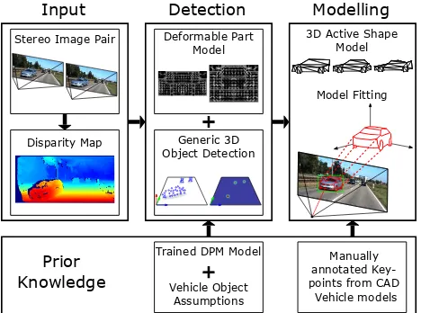
The whole framework is depicted in Fig. 1. After 3D recon-struction, the proposed procedure is divided into two main parts: Thedetectionstep, which delivers 3D vehicle detections and the modellingstep, in which a vehicle model is fitted to the detected objects. In the detection step we make use of both, the 3D data as well as the image data by fusing a generic 3D object detector with an object specific vehicle detector to obtain reliable vehicle detections. In the modelling step we try to fit a 3D deformable vehicle model to each of the vehicle detections. The different steps are explained in more detail in the subsequent sections.
Deformable Part Model
Generic 3D Object Detection
Input Detection Modelling
Stereo Image Pair
Disparity Map
3D Active Shape Model
Model Fitting
Prior Knowledge
Trained DPM Model
Vehicle Object Assumptions
Manually annotated Key-points from CAD
Vehicle models
Figure 1. High-level overview of our framework.
3.1 Problem statement
Let each scene be described by a ground planeΩ ∈ R3 and a set of vehicle objectsOthat are visible in the respective stereo image pair. Each vehicle objectok ∈ Ois represented by its
state vector(xk,tk, θk, γk). xkis the set of reconstructed 3D object points belonging to the vehicle, i.e. lying on the visible surface of the vehicle. tkandθkdetermine the pose of the ve-hicle, with the positiontkrepresented by 2D coordinates on the
ground plane, whereasθkis the rotation angle about the axis ver-tical to the ground plane (heading).γkare shape parameters de-termining the shape of a 3D deformable vehicle model associated to each object. In this context, we use a 3D active shape model (ASM) (Zia et al., 2013). More details on the vehicle model and the shape parameters can be found in Sec. 3.3.
Given the left and right stereo images, the derived disparity im-age and the reconstructed point cloud, the goal of our proposed method is to detect all visible vehicles and to determine the state parameters listed above for each of the detected vehicles.
3.2 Detection of vehicles
The goal of this step is to detect all visible vehiclesok in the
stereo image pair by finding their corresponding 3D object points
xkand initial values for the pose parameters0tk and0θk. By
using street level stereo images obtained from a moving vehicle, a set of plausible assumptions can be made and incorporated into the vehicle detection procedure. The stereo camera is mounted on the car at a fixed height above ground and the car moves on a planar street surface, acquiring the stereo image sequence in an approximately horizontal viewing direction. Besides, we build our method on the following assumptions for vehicles:
i) Vehicles are located on the street, i.e. on the ground plane ii) Vehicles are surrounded by free space
iii) Vehicles have a maximum heighthmax
iv) Vehicles have a minimum and a maximum area that they cover on the ground
Taking into account these assumptions, the detection framework is divided into the following steps: We use the disparity and 3D information to detect and extract the 3D ground plane. Subse-quently we detect generic 3D objects as clusters of projected 3D points on that ground plane and use them to generate vehicle hy-pothesis. To verify the vehicle hypothesis, we additionally apply a state-of-the-art vehicle detector to the reference stereo image. The different processing steps are explained in more detail in the following paragraphs.
3.2.1 Ground plane extraction: Working with street level stereo images, the ground plane can be extracted in the so called v-disparity image (Zhu et al., 2013), which is a row-wise dis-parity histogram: Given the disdis-parity map, the v-disdis-parity image is obtained by accumulating the pixels with the same disparity that occur on the respective image line. In the v-disparity im-age, the ground plane is represented by a straight line. As street level stereo images typically contain a lot of pixels belonging to the ground, the ground correlation line in the v-disparity image results in large histogram entries. We detect that ground correla-tion line by applying RANSAC to determine the line parameters of the Hesse normal form. All pixels in the v-disparity image that contribute to the ground correlation line can be backprojected to the disparity image so that the image regions showing the ground plane can be identified. The 3D points reconstructed from the pixel disparities belonging to the ground plane region are used to determine a 3D ground plane in the model coordinate system as the best fitting planeΩ:
Ω :ax+by+cz+d= 0, (1)
wherev= [a b c]T with||v||= 1is the normal vector anddis
the offset of the plane.
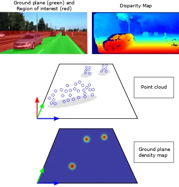
compute a density map of the 3D points. To this end, we define a grid with a cell widthwgridin the ground plane. Each grid cell then contains a scalar value representing the number of points falling into that cell. In each cell, we also store a list of associ-ated 3D points and 2D pixel indices. Following assumption ii), each vehicle corresponds to a cluster of projected 3D points in the ground plane density map (see Fig. 2). We apply Quick-Shift Clustering (Vedaldi and Soatto, 2008) as a mode seeking tech-nique to identify the different clusters. An object hypothesis is represented by a set of cells that converged to the same cluster mode and is composed of the set of 3D pointsxk associated to the respective cluster cells. The stored set of image pixel indices is used to derive a 2D bounding boxBBimgk for each object in image space.
As our object detection technique delivers generic object propos-als, the list of detected objects will still contain non-vehicle ob-jects, such as persons, poles, or street furniture. According to assumption iv), vehicles also have a certain minimum and maxi-mum area. Thus, we define a minimaxi-mum and maximaxi-mum threshold
AminandAmaxas lower and upper boundaries for a valid size of the 2D bounding box on the ground plane and discard object pro-posals that fall belowAminor exceedAmaxto reject presumed non-vehicle objects. The result is a set of vehicle object hypothe-ses which will be introduced to a subsequent verification step as described in Sec. 3.2.3.
Ground plane (green) and
Region of interest (red) Disparity Map
Point cloud
Ground plane density map
Figure 2. Detection of generic object proposals.
3.2.3 Verification of vehicle hypotheses: Applying our generic object detection technique, we make two observations: Firstly, generic object detection results in a large completeness for vehi-cles with the drawback of a large amount of false alarms. Sec-ondly, we achieve a considerable amount of multiple detections for the same vehicle. Caused by cluttered and/or incomplete dense matching results, the projections of the 3D points of a ve-hicle to the ground plane may result in multiple clusters in the density map, thus leading to multiple vehicle hypotheses for a single object. To counteract these problems, we combine our generic detection technique with an object specific detector to obtain our final vehicle detections. To this end, we make use of the DPM defined by Felzenszwalb et al. (2010), which uses an object-specific part-based model to detect objects based on HOG features. The DPM delivers 2D image bounding box detections
BBDP M
l which we use to verify the vehicle hypotheses resulting
from our 3D vehicle detection technique. We compute the Jac-card IndexJ(BBkimg, BBDP M
l ), which equals the intersection over union index, for the bounding boxesBBkimgand the DPM bounding boxesBBDP M
l . We only keep detections that are sup-ported by a DPM detection, i.e. we keep a vehicle hypothesis only if there is a DPM detection withJ(BBkimg, BB
DP M l )> τ and discard all other object hypotheses. τ is a threshold which has to be defined by the user. Additional to the rejection of non-vehicle object detections, we use the DPM bounding boxes to merge multiple detections from the generic object detector when theirBBimgk bounding boxes have a Jaccard Index> τ for the sameBBDP M
l bounding box.
The remaining final vehicle detections are used as initial objects 0o
k = (xk,0tk,0θk,0γk)in the model fitting step. We deter-mine the ground plane bounding boxesBBGP
k for each vehicle as the rectangle of the minimum area enclosing the object points
xkprojected on the ground plane. We make use ofBBkGPto
ini-tialize the pose parameters0tkand0θk: We define0tkas the 2D
position of the bounding box center on the ground plane and0θk as the direction of the semi-major axis of the bounding box. The shape parameter vectors0γk are initialised as zero vectors0T. As described in Sec. 3.3, the initial vehicle model thus is defined as the mean vehicle model.
3.3 3D Modelling
Given the initial vehicle detections, our aim is to find an object specific vehicle model for each detected object that describes the object in the stereo images best in terms of minimizing the dis-tance between the observed 3D object pointsxk and the model surface. For that purpose, we make use of a 3D active shape model (ASM) as in (Zia et al., 2013). Similar to (Zia et al., 2013), our ASM is learned by applying principal component analysis (PCA) to a set of manually annotated characteristic keypoints of 3D CAD vehicle models. By using vehicles of different types (here: compact car, sedan, estate-car, SUV and sports-car) in the training set, the PCA results in mean values for all vertex (key-point) positions as well as the directions of the most dominant vertex deformations. A deformed vehicle ASM is defined by the deformed vertex positionsv(γk)which can be obtained by a
lin-ear combination
v(γk) =m+X
i
γk(i)λiei (2)
of the mean modelmand the eigenvectorsei, weighted by their corresponding eigenvalues λiand scaled by the object specific shape parameters γ(i)k . The variation of the low dimensional shape vectorγk thus allows the generation of different vehicle shapes. Fig. 3 shows the mean model and two deformed model using a different set of shape parameters. Note how the shape pa-rameters enable the generation of model shapes describing vehi-cles of different categories or types. For the number of the eigen-values and eigenvectors to be considered in the ASM we choose
i∈ {1,2}, as we found this to be a proper tradeoff between the complexity of the model and the quality of the model approxima-tion.
In order to fit an ASM to each of our vehicle detections, we define a triangular mesh for the ASM vertices (see Fig. 3) and trans-late and rotate the model on the detected ground plane according to the object posetk andθk, respectively. Similar to (Xiao et
al., 2016), we aim to find optimal values for the variablestk,θk
Figure 3. 3D Active Shape Models. Center: mean shape,
γ= (0,0)and two deformations, left:γl= (1.0,0.8), right:
γr= (−1.0,−0.8)
pointsxkto the triangulated surface of the transformed and de-formed active shape modelM(tk, θk, γk)becomes minimal. For
that purpose, we apply an iterative approach: As the model pa-rameters are continuous we discretise the papa-rameters and gener-ate model particles for the ASM by performing informed param-eter sampling to reduce the computational expense. Starting from the initial parameters0tk,0θk,0γk, we generatenpparticles in each iterationj = 0...nit, jointly sampling pose and shape pa-rameters from a uniform distribution centered at the solution of the preceding particle parameters. In each iteration, we reduce the respective range of the parameters and keep the best scoring particle to use it to define initial values in the subsequent iteration. The score, which is defined as an energy term
Ek(tk, θk, γk) = 1 P ·
P
X
p=1
d(pxk, M(tk, θk, γk)), (3)
corresponds to the mean distance of thePvehicle pointspxk∈
xkfrom the surface of the model corresponding to a particle and
has to become minimal. In Eq. 3,d(·, ·)is a function that cal-culates the distance of an individual 3D vehicle point from the nearest model triangle. The best scoring particle of the last itera-tion is kept as final vehicle model and the vehicle pose relative to the observing vehicle can be derived from the model parameters directly.
4. EVALUATION 4.1 Parameter settings
Our vehicle detection and modelling setup requires the definition of several parameters. For the 3D reconstruction, the maximal valueδσZ for the precision of the depth values is defined as 1.5 [m]. For the calibration parameters of the stereo cameras used for acquiring the data (see Sec. 4.2), this leads to a minmum valid disparity of 16 [px] and thus, a maximum distance of the 3D points from the camera of 24.3 [m].
The parameters for the generic object detection approach are set tohmax= 3.5 [m]andAmin= 1.0 [m2]andAmax= 9.0 [m2] as lower and upper boundary thresholds for the object area on the ground plane. The DPM verification thresholdτ is defined empirically and is set toτ= 0.5.
For the model fitting procedure we conduct a number ofnit= 12 iterations while drawingnp = 100particles per iteration. As initial interval boundaries of the uniform distributions from which we randomly draw the particle parameters, we choose±1.5[m] for the location parametertk,±1.0for the shape parameterγk
and±180◦for the orientationθ
k. By choosing±180◦as interval for the orientation angle, we allow particles to take the whole range of possible orientatios in the first iteration to be able to deal with wrong initialisations. In each iterationj the interval boundaries are decreased by the factor0.9j
. Withnit = 12, this leads to a reduction of the interval range in the last iteration to 28% of the initial interval boundary values.
4.2 Test data and test setup
For the evaluation of our method we use stereo sequences of the KITTI Vision Benchmark Suite (Geiger et al., 2012). The data were captured by a mobile platform driving around in urban ar-eas. We make use of the object detection and object orientation estimation benchmark which consists of 7481 stereo images with labelled objects. In our evaluation we consider all objects la-belled ascar. For every object, the benchmark provides 2D image bounding boxes, the 3D object location in model coordinates as well as the rotation angle about the vertical axis in model coordi-nates. Furthermore, information about the level of object trunca-tionand objectocclusionare available. The values fortruncation
refer to the objects leaving image boundaries and are given as float values from 0 (non-truncated) to 1 (truncated) while the oc-clusion state indicates the vehicle ococ-clusion due to other objects with 0 = fully visible, 1 = partly occluded, 2 = largely occluded and 3 = unknown.
We evaluate our approach concerning the results forobject detec-tionas described in Sec. 3.2 and concerning the results forpose estimationto analyse the quality of our model fitting approach as described in Sec. 3.3. For the evaluation ofobject detection, sim-ilarly to (Geiger et al., 2012), we define three level of difficulties as shown in Tab. 1: easy,moderateandhard, each considering different objects for the evaluation, depending on their level of visibility.
easy moderate hard min. bounding box height [Px] 40 25 25
max. occlusion level 0 1 2
max. truncation 0.15 0.30 0.50
Table 1. Levels of difficulties as evaluation criteria.
As defined by (Geiger et al., 2012), we require an overlap of at least 50% between the detected 2D bounding box and the refer-ence bounding box to be counted as a correct detection in our evaluation. In the case of multiple detections for the same ve-hicle, we count one detection as a true positive, whereas further detections are counted as false positives.
For the evaluation of thepose estimationwe consider all correctly detected vehicles and compare the 3D object locationstk and
the orientation anglesθkof our fitted models, both with respect to the model coordinate system, to the provided reference posi-tions and orientaposi-tions. We consider a model to be correct in pose and/or orientation, if its distance from the reference position is smaller than 0.75 [m] and the difference in orientation angles is less than 35.0◦, respectively. With regard to the quality of the reconstructed 3D points, we consider these definitions as proper values for the evaluation.
4.3 Vehicle detection results
Tab. 2 shows the number of reference objects (#Ref) and the resulting numbers of correctly (#TP) and falsely (#FP) detected objects, as well as the number of missed objects (#FN) result-ing from processresult-ing the whole evaluation data set. Further, we calculate values for (Heipke et al., 1997)
Completeness [%]= 100· #T P
#T P+ #F N, (4)
Correctness [%]= 100· #T P
Quality [%]= 100· #T P
Completeness [%] 86.5 77.5 63.4 Correctness [%] 86.3 90.6 91.7 Quality [%] 76.1 71.8 60.0
Table 2. Vehicle detection results.
For theeasydetection level, i.e. regarding only vehicles which are fully visible in the reference stereo image, we are able to achieve satisfying detection results by detecting more than 86% of all vehicles while achieving a value for the correctness that is also larger than 86%. As is apparent from Tab. 2, our detec-tion approach has increasing difficulties to detect vehicles with increasing occlusion and/or truncation states. This is why the values for completeness decrease for the evaluation levels mod-erateandhard. However, the number of false positive detections remains constant. As our approach only detects the vehicle parts visible in both stereo images, whereas the reference bounding boxes contain also the non-visible object parts, the difference be-tween detection and reference bounding boxes will increase with increasing degree of occlusion. As a consequence, a certain ex-tent of detections counted as false positive may de facto be correct vehicle detections.
4.4 Pose estimation results
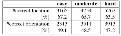
Tab. 3 shows the results of the comparison between the resulting pose parameters of the fitted 3D vehicle models and the reference data for location and orientation of the vehicles. Here only the correctly detected vehicles are considered in the evaluation.
easy moderate hard #correct location 3165 4754 5267
[%] 67.2 65.7 63.5
#correct orientation 2313 3511 3913
[%] 49.1 48.5 47.2
Table 3. Pose estimation results.
Regarding the easyevaluation level, our model fitting strategy leads to 67.2% of correct location estimations and to 49.1% of correct orientation results. The two tougher evaluation levels lead to slightly decreased values for both, the location as well as the orientation. While the position estimation results are encourag-ing, the results of the orientation estimates are not yet satisfying.
To get a more detailed interpretation of the orientation results, Fig. 4 shows a histogram of vehicle detections for several classes of orientation differences between the orientation derived by our method and the reference orientation. From this histogramm it is apparent that the distinct majority of the false model orientations have a difference to the reference orientation between 157.5◦and 180◦, i.e. our fitted model very often results in a more or less op-posed direction compared to the true direction. On the one hand, the reason for that may be found in the way the model tion is initialized. As initial orientation we compute the orienta-tion of the larger semi-half axis of the object’s bounding box on the ground plane. Due to that, the model initialisation has two
≤22.5
Figure 4. Histogram of absolute differences between model orientation and reference object orientation.
possibilities of opposing orientation directions. We try to com-pensate for that initialisation error by accepting orientations in the range of±180◦in the first iteration step. On the other hand, some vehicles may be seen as being approximately symmetric in 3D not only with respect to their major but also with respect to their minor half axis. Especially when using noisy stereo image point clouds, the shapes defined by the 3D points of the front and the back side of a car might not be discriminative enough to fit the vehicle model into the set of 3D points correctly. The vehi-cle symmetry thus might lead to a local minimum of the mean distance between the 3D points and the vehicle particles with an opposed orientation.
Some results of our model fitting approach are shown in Fig. 5 by backbrojecting the resultant wireframes to the reference image. While the first three rows show some successful model fitting examples, the last three rows exhibit some typical failure cases. On the one hand, the above discussed model fitting errors with an orientation offset of±180◦become apparent. Additionally, another problem becomes obvious: Vehicles observed directly from behind lead to fitted models with an orientation offset of ±90◦. The reason for that might be, that the available 3D points for these cars only describe the vertical backside of the vehicle. As a consequence, this leads to problems for the orientation ini-tialisation due to a more or less one dimensional bounding box on the ground plane and due to fitting ambiguities between the 3D points and the vehicle model.
5. CONCLUSION
Figure 5.Qualitative results:backprojected wireframe of the fitted vehicle models. First three rows: positive examples, last three rows: typical examples of errors
of estimated orientations correspond to the opposed viewing di-rection. We suspect this problem might be caused by model ini-tialisation problems combined with the symmetric shape of some vehicles. To overcome these problems, we want to enhance our model fitting approach in the future. On the one hand we want to introduce a bimodal or even multimodal distribution to draw the model orientation parameter from. Secondly, the tracking of several particles instead of only keeping a single particle in each iteration could also lead to better results. Moreover, the model fitting currently only builds on the 3D stereo information. In fu-ture developments we also want to introduce image information into the model fitting approach, e.g. by also taking into account the alignment of image edges and model edges.
ACKNOWLEDGEMENTS
This work was supported by the German Research Founda-tion (DFG) as a part of the Research Training Group i.c.sens [GRK2159].
References
Chen, X., Kundu, K., Zhu, Y., Berneshawi, A. G., Ma, H., Fidler, S. and Urtasun, R., 2015. 3d Object Proposals for accurate Object Class Detection. In: Advances in Neural Information Processing Systems, Vol. 28, pp. 424–432.
Cootes, T., Baldock, E. and Graham, J., 2000. An Introduction to Active Shape Models. In:Image Processing and Analysis, pp. 223–248.
Engelmann, F., St¨uckler, J. and Leibe, B., 2016. Joint Object Pose Estimation and Shape Reconstruction in Urban Street Scenes Using 3D Shape Priors. In:Pattern Recognition, Lecture Notes in Computer Science, Vol. 9796, pp. 219–230.
Geiger, A., Lenz, P. and Urtasun, R., 2012. Are we ready for autonomous Driving? The KITTI Vision Benchmark Suite. In: 2012 IEEE Conference on Computer Vision and Pattern Recognition (CVPR), pp. 3354–3361.
Geiger, A., Roser, M. and Urtasun, R., 2011. Efficient Large-Scale Stereo Matching. In: Computer Vision – ACCV 2010, Lecture Notes in Computer Science, Vol. 6492, pp. 25–38.
Han, F., Shan, Y., Cekander, R., Sawhney, H. S. and Kumar, R., 2006. A two-stage Approach to People and Vehicle Detection with HOG-based SVM. In: Performance Metrics for Intelli-gent Systems 2006 Workshop, pp. 133–140.
Heipke, C., Mayer, H., Wiedemann, C. and & Jamet, O., 1997. Evaluation of automatic Road Extraction. In: International Archives of Photogrammetry and Remote Sensing, Vol. 32, pp. 151–160.
Leibe, B., Leonardis, A. and Schiele, B., 2006. An Implicit Shape Model for combined Object Categorization and Segmentation. In:Toward Category-Level Object Recognition, Lecture Notes in Computer Science, Vol. 4170, pp. 508–524.
Liebelt, J. and Schmid, C., 2010. Multi-view Object Class Detec-tion with a 3D geometric Model. In:2010 IEEE Conference on Computer Vision and Pattern Recognition (CVPR), pp. 1688– 1695.
Menze, M., Heipke, C. and Geiger, A., 2015. Joint 3d Estima-tion of Vehicles and Scene Flow. In: ISPRS Annals of the Photogrammetry, Remote Sensing and Spatial Information Sci-ences, Vol. II-3, pp. 427–434.
Osep, A., Hermans, A., Engelmann, F., Klostermann, D., Math-ias, M. and Leibe, B., 2016. Multi-scale Object Candidates for generic Object Tracking in Street Scenes. In: 2016 IEEE In-ternational Conference on Robotics and Automation (ICRA), pp. 3180–3187.
Ozuysal, M., Lepetit, V. and Fua, P., 2009. Pose Estimation for Category specific Multiview Object Localization. In: 2009 IEEE Computer Society Conference on Computer Vision and Pattern Recognition Workshops (CVPR Workshops), pp. 778– 785.
Payet, N. and Todorovic, S., 2011. From Contours to 3D Object Detection and Pose Estimation. In:2011 IEEE International Conference on Computer Vision (ICCV), pp. 983–990.
Pepik, B., Stark, M., Gehler, P. and Schiele, B., 2012. Teaching 3D Geometry to deformable Part Models. In:2012 IEEE Con-ference on Computer Vision and Pattern Recognition (CVPR), pp. 3362–3369.
Thomas, A., Ferrari, V., Leibe, B., Tuytelaars, T. and van Gool, L., 2007. Depth-From-Recognition: Inferring Meta-data by Cognitive Feedback. In: 2007 IEEE 11th International Con-ference on Computer Vision (ICCV), pp. 1–8.
Vedaldi, A. and Soatto, S., 2008. Quick Shift and Kernel Methods for Mode Seeking. In:Computer Vision – ECCV 2008, Lecture Notes in Computer Science, Vol. 5305, pp. 705–718.
Villamizar, M., Grabner, H., Moreno-Noguer, F., Andrade-Cetto, J., van Gool, L. and Sanfeliu, A., 2011. Efficient 3D Object Detection using Multiple Pose-Specific Classifiers. In:British Machine Vision Conference 2011, pp. 20.1–20.10.
Xiao, W., Vallet, B., Schindler, K. and Paparoditis, N., 2016. Street-Side Vehicle Detection, Classification and Change De-tection using mobile Laser Scanning Data. ISPRS Journal of Photogrammetry and Remote Sensing114, pp. 166–178.
Zhu, X., Lu, H., Yang, X., Li, Y. and Zhang, H., 2013. Stereo Vision based traversable Region Detection for mobile Robots using u-v-disparity. In:Proceedings of the 32nd Chinese Con-trol Conference, pp. 5785–5790.
Zia, M. Z., Stark, M. and Schindler, K., 2015. Towards Scene Understanding with Detailed 3D Object Representations. In-ternational Journal of Computer Vision112(2), pp. 188–203.
Zia, M. Z., Stark, M., Schiele, B. and Schindler, K., 2011. Re-visiting 3D geometric Models for accurate Object Shape and Pose. In:IEEE International Conference on Computer Vision Workshops (ICCV Workshops), pp. 569–576.