COSEISMIC DEFORMATION FIELD AND FAULT SLIP DISTRIBUTION OF THE 2015
CHILE Mw8.3 EARTHQUAKE
Qu Chunyan*, Zuo Ronghu, Shan XinJian, Zhang Guohong, Zhang Yingfeng, Song Xiaogang
State Key Laboratory of Earthquake Dynamics, Institute of Geology, China Earthquake Administration, Beijing, 100029, China - [email protected], (zuorh, xjshan, zhanggh, zhangyf, songxg)@ies.ac.cn
ThS 5
KEY WORDS: Chile earthquake, InSAR, coseismic deformation, slip distribution, inversion
ABSTRACT:
On September 16, 2015, a magnitude 8.3 earthquake struck west of Illapel, Chile. We analyzed Sentinel-1A/IW InSAR data on the descending track acquired before and after the Chile Mw8.3 earthquake of 16 September 2015. We found that the coseismic deformation field of this event consists of many semi circular fringes protruding to east in an approximately 300km long and 190km wide region. The maximum coseismic displacement is about 1.33m in LOS direction corresponding to subsidence or westward shift of the ground. We inverted the coseismic fault slip based on a small-dip single plane fault model in a homogeneous elastic half space. The inverted coseismic slip mainly concentrates at shallow depth above the hypocenter with a symmetry shape. The rupture length along strike is about 340 km with maximum slip of about 8.16m near the trench. The estimated moment is 3.126×10²¹ N.m Mw8.27 ,the maximum depth of coseismic slip near zero appears to 50km. We also analyzed the postseismic deformation fields using four interferograms with different time intervals. The results show that postseismic deformation occurred in a narrow area of approximately 65km wide with maximum slip 11cm, and its predominant motion changes from uplift to subsidence with time. that is to say, at first, the postseismic deformation direction is opposite to that of coseismic deformation, then it tends to be consistent with coseismic deformation.It maybe indicates the differences and changes in the velocity between the Nazca oceanic plate and the South American continental plate.
* Corresponding author
1. INTRODUCTION
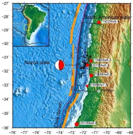
On September 16, 2015, a magnitude of Mw8.3 earthquake struck off shore of Chile and induced tsunami http://earthquake.usgs.gov/). This huge event occurred on the
subduction zone between the Nazca and South America plates in Central Chile, with the epicenter about 85 km distant to the Chile trench(Figure 1). At the latitude of this event, the Nazca plate is moving towards the east-northeast at a rate of 65-74 mm/yr with respect to South America, and begins its subduction beneath the continental South American plate at the Peru-Chile
trench http://earthquake.usgs.gov/earthquakes/). The Chile
subduction zone is one of the most prone to earthquakes in the world. The 2010 Mw8.8 Maule earthquake which is located about 400km south of the 2015 event in central Chile ruptured a
~600 km long section of the plate boundary(Tong, 2010,
Delouis, 1997,2009,2010;Fred , 2011;Bertrand, 2010).
In this paper, we use Sentinal-1A/IW InSAR data to map the coseismic deformation field the Mw8.3event and invert the spatial variations of fault slip. Meanwhile, we use four SAR images acquired at different times after the mainshock to reveal the pattern and variation of the short-term post-seismic
deformation. Finally we make some interpretation and discussion to the observation and inversion results.
earthquake rupture zones. ETOPO1 Digital Elevation Models are used to generate the background topography and bathymetry. The black rectangle is the fault plane projected onto the surface.
2. INSAR DATA AND PROCESSING
We investigate the coseismic and postseismic deformation fields produced by the 2015 Mw8.3 Chile earthquake using InSAR data from Sentinel-1A/IW on descending orbit. Just on the second day after the earthquake, the satellite Sentinel-1A acquired descending data covering the whole seismic area. Because very close to the mainshock time, these data permit to study the coseismic deformation of this event avoiding influences of short-term post earthquake deformation and aftershocks. We downloaded these data as well as those before the event and generated the coseismic interferograms. We used three adjacent senses on the same track to cover the whole deformation field along the coast. Meanwhile, we used four SAR images acquired at different dates after the main shock and construct four interferograms to study the spatial distribution and temporal evolution of short-term post-seismic deformation. The SAR data and its parameters used in the paper are shown in Table 1.
No Track Master Slave B⊥ (m)
T(day)
3 D 20150707 20150917 -3 72 4 D 20150917 20151011 6 24 5 D 20150917 20151023 11 36 6 D 20151011 20151023 5 12 7 D 20151011 20151104 57 24
Table 1. Sentinel-1A/IW data used in this article
We used the GAMMA software to process the Sentinel-1A InSAR data, we firstly generated coseismic interferograms separately for each of the three adjacent image pairs on the same track, and then integrated them to produce a large interferogram to cover the whole coseismic deformation area. In the processing, we removed topographic phase by generating simulated interferogram using SRTM DEM. To reduce noise, multi-look processing of 10-sight in range and 2-sight in azimuth directions was performed to the interferograms. Meanwhile, the adaptive filters based on interferometric fringe frequency and gradually decreasing windows were applied to interferograms so that the ratio of signal to noise was highly enhanced, fringes associated with seismic deformation were highlighted, and phase unwrapping was easy to proceed. The algorithm of minimum cost flow for phase unwrapping (provided by the GAMMA software) was adopted, which is based on the Delaunay triangle network and suitable for areas of low coherence. It should be mentioned that the interferometric processing with Sentinel-1A/IW data requires a very high registration accuracy nearly 0.1/% of an SLC pixel especially in the azimuth direction,so we performed iterating offset
estimation for many times until the azimuth offset correction became at least smaller than 0.02 SLC pixel to make sure to get the clear deformation fringes. Using similar data processing methods, we dealed with postseismic InSAR data and acquired the variation and distribution of the postseismic deformation.
3. COSEISMIC DEFORMATION FIELDS FROM SENTINEL-1A INSAR DATA
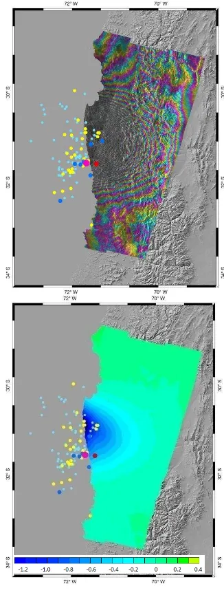
The entire coseismic deformation field generated by integrating three neighbour interferograms on the same descending track is shown in Figure 2, which covers almost the whole affected area of the 2015 Chile earthquake. It consists of dense concentric semi-circular fringes convex to east, the dominant motion direction is subsidence of LOS(moving away from the satellite), meaning the South American plate westward movement. Furthermore, the more close to the coast, the more dense the fringe, implying increasing deformation gradient. The maximum LOS subsidence reaches about 133cm near the coast.
Figure 2. up: Coseismic interferogram of Mw8.3 mainshock from Sentinel-1A/IW data on descending track. Down: The corresponding unwrapped interferometric displacement. A fringe indicates 28cm LOS displacement. Big pink dot is the epicenter of Mw8.3 mainshock, other color dots show aftershocks from http://earthquake.usgs.gov, as of 18/9/2015 (red dot: Mw>7.0, blue dots:7.0 >Mw>6.0, yellow dots:6.0 >Mw>5.0, cyan dots:5.0 >Mw>4.0),white dashed lines indicate the profile location
4. POST-SEISMIC DEFORMATION FIELDS FROM SENTINEL-1A INSAR DATA
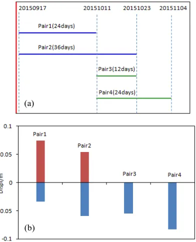
We use four image pairs to generate interferograms to study the spatial distribution and temporal evolution of short-term post-seismic deformation of the 2015 Chile great event. These pairs are named pair 1 20150917_20151011 , pair 2
20150917_20151023 , pair 3 20151011_20151023 and
pair 4 20151011_20151104 , respectively. All of these
interferograms have the roughly same coverage, i.e. the scene of the central coseismic interferogram which covers most of the deformation area of the mainshock. Figure3(a) shows time spans of the four interferograms(pairs) and dates of image acquisitions. Figure3(b) displays LOS displacements from these interferograms, which indicate uplift and sink in LOS direction for the pair 1 and pair 2, whereas only sink for the pair 3 and pair 4. The differences of these interferograms having different time intervals reflect variations of post-seismic deformation with time.
Figure 3. (a) Schematic showing the time spans of the four post-seismic SAR image pairs. Dotted vertical lines are SAR image acquisition dates. Red vertical line shows the date of the
mainshock. Color horizontal lines are time intervals of the four pairs. (b) Maximum post-seismic displacements in LOS direction derived from the four interferograms. The vertical axis represents the displacement in meter.
4.1 Post-seismic deformation from pair1 and pair2
SAR image pair 1 and pair 2 share the same master image which was acquired one day after the main shock (17 September 2015),while their slave images were acquired on the 24th and 36th day after the main shock. From the interferograms of these two pairs (Figure4), both reveal the largely same post-seismic deformation fields. The post displacements are distributed in a 65km-wide zone along the coast(white dashed lines in Figure4(a)), and those beyond 65km are as small as less than ±2cm which have large local variations without tendency of phase change, thus considered noise. The post-seismic deformation includes uplift and sink in LOS direction, i.e. a relatively large uplifted area in the south and a small subsidence area in the north. From pair 1, the maximum uplift is 7cm and maximum sink 4cm, implying relative deformation 11cm (Figure4(a), (b)). From pair 2, these values are 5cm, 6cm, and 11cm, respectively (Figure4(c), (d)). The location of large displacement coincides with the main shock, 70-75km north of the instrumental epicenter. These two interferograms reveal the post-seismic deformation at nearly one-month scale. It is commonly thought that the deformation one month or even one to two years after the mainshock is afterslip produced by the unruptured part of the causative fault plane with same motion sense as the main shock (Tan et al., 2005; Vigny, et al., 2011). However, the short-term post-seismic deformation revealed by the two inetrferograms above seems complicated. First, it is opposite in motion direction with the main shock, thus cannot be explained by post-seismic slip on the fault plane. Second, on the same covered area, the whole coseismic field is a half-circle subsidence area concaving toward east, without uplift (Figure4(e), (f)), while the post-seismic deformation field extends along the coast or the rupture zone with both uplift and subsidence (Figure 4(a)-(d); Figure.3 (b)). Such a contrast is interest but elusive, which will be discussed later.
(a)
Figure 4. (a) and (b) Post-seismic interferogram of pair 1 (0917_1011) and its unwrapped displacement, (c) and (d) Post-seismic interferogram of pair 2 (0917_1023) and its corresponding unwrapped displacement, (e) and (f) Coseismic interferogram and its unwrapped displacement in the same area for comparison. A fringe indicates 2.8cm LOS displacement. Big pink dot is the epicenter of Mw8.3 mainshock, other color dots show aftershocks with implication same as in Figure2.
4.2 Post-seismic deformation from pair3 and pair4
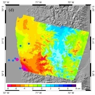
The master image of pairs 3 and 4 is 20151011, i.e. the 24th day after the mainshock; while their slave images were acquired on the 36th day (20151023) and 48th day (20151104) after the event, respectively. The post-sesimic deformation field scope (Figure5) is largely consistent with that of pairs 1 and 2 stated in the last section, also distributed in a 60-65km-wide zone (a)
(c)
(e) (f)
(b)
along the coast. But the overall deformation amount is relatively smaller, and of negative values, implying LOS subsidence or westward motion of the land, in agreement with the main shock but opposite to that from pairs 1 and 2. It is noted that the subsidence from pair 4 is the largest (about 8cm), greater than that from pair 3 (about 4cm). As time going on, the post-seismic LOS subsidence accumulated and tended to increase, which can be explained by the afterslip model.
Figure 5. (a) and (b) The post-seismic interferogram from SAR image pair 3 (1011_1023) and its corresponding unwrapped interferometric displacement. (c) and (d) The post-seismic interferogram from SAR image pair 4 (1011_1104) and its corresponding unwrapped interferometric displacement. A fringe indicates 28cm LOS displacement. Big pink dot is the epicenter of Mw8.3 mainshock, other color dots show aftershock with implication same as in Figure2
5. COSEISMIC SLIP INVERSION
We used InSAR observations to constrain a model of coseismic slip on a single plane fault in elastic half-space. The geometry of the fault plane was initially determined according to focal mechanism solutions given by USGS and GCMT (http://www.usgs.gov/), and then refined using the InSAR deformation data. The fault surface trace follows the trench axis. We resampled the InSAR deformation field by the quad-tree resampling method to get a lower resolution dataset for inversion (Jónsson, 1999). Finally, we have 12763 sampled points for inversion. A linear inversion method called Sensitivity Based Iterative Fitting (SBIF) method was employed (Wang, 2008). Firstly, the fault plane was divided into multiple fault patches. Each patch was presumed to slip uniformly. In this way, the non-linear problem can be transformed into a linear problem. Then we designed a mean square deviation reducing function to evaluate the fitting effect between the simulated interferogram and the observed one. Using this function, we obtained the minimum value of mean square deviation, and finally acquired the non-uniform slip distribution on the fault plane.
Our inversion results indicate that the preferred slip model (Figure6) shows a concentrated fault rupture zone located in the shallow part of the up-dipping thrust fault above the hypocenter. The maximum fault slip is over 8m at a shallow depth above 9km, located in the northwest of the epicenter. This is (a)
(c) (b)
consistent with the large LOS displacement in the region seen in the interferograms(Figure2). The slip is gradually decreasing to the deep subsurface and the north and south sides along the fault strike. Slip in the Chile trench is large and reaches about 8m. The boundary of the rupture zone is relatively clear with a shape of symmetric pattern along fault strike, the depth at which the coseismic slip drops to zero is variable along rupture zone. The maximum depth where slip can be ignored is nearly 50km under the surface. The rupture length of the slip area is about 340km along fault strike, comparable with 335 km of the major axis of aftershock distribution in this direction. But the slip mainly distributed in the shallow part above 15km depth and 200 km long on the subduction interface. The mean rake angle from inversion is 116.4°, consistent with the thrust fault motion. The simulated interferogram is reconciled well with the observed one with maximum residual ~0.05m. The fitting degree of the whole field is 99.97. The seismic moment magnitude is Mw8.27,which consistent with focal mechanism solutions from seismic waves (Mw=8.2,GCMT;
Mw=8.3,USGS . It indicates that our inversion results are
reliable. .
Figure 6. Coseismic slip distribution model derived from this inversion displaying in 3D frame. Red star symbol indicates the Global CMT epicenter.
6. DISCUSSION
It is interesting to probe the down-dip limit of the seismogenic zone and the transition depth from seismic to aseismic slip of thrust faulting earthquakes on the Chile subduction zone. Inversion of the co-seismic rupture depth constrainted by a dense InSAR data can provide evidence to address this issue. Some researchers have inverted the rupture depth of the 2010 Chile Mw8.8 event using InSAR and GPS data.Tong et al,(Tong,2010 estimated the maximum rupturing depth of this event to be 43-48km from ALOS/PALSAR and GPS data. Fred et al. (Fred,2011) suggested that the fault rupture of this event terminated at a depth of 35km, also based on joint inversion of ALSO/PALSAR and GPS data, which seems shallow, likely associated with the spherical layering Earth model used in the inversion. Delouis et al. (Delouis,2010) constrained the maximum down-dip depth as 50km for the 2010 Chile great
shock by joint inversion of teleseismic records, InSAR and high rate GPS (HRGPS) data.
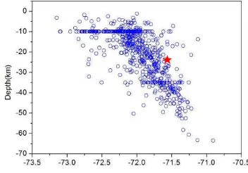
Our model constrained by InSAR data requires a maximum rupture depth of the 2015 Mw8.3 event be 50-55km (Figure6). This value is roughly consistent with the previous results estimated from 2010 Mw8.8 event, also in agreement with the maximum depth of the aftershock distribution (Figure 7).
Figure 7. Distribution of aftershock depths in the direction of longitude (aftershocks from http://earthquake.usgs.gov, as of 11/10/2015), Red stars indicate the Global CMT epicenter of mainshock.
These features of post-seismic deformation are likely associated with the tectonic setting of the 2015 Chile great earthquake. The Nazca plate is underthrusting beneath the South American plate, probably the former is dominant or active, causing relative motion between the two plates. Although the westward motion of the American continental plate is observed by InSAR, the displacement of the Nazca oceanic plate in the west must be greater than that within the continent to east, though which cannot be measured due to coverage of sea water. The zone-like post-seismic deformation, opposite to the coseismic, is probably due to the larger motion rate of the Nazca plate in a short time after the mainshock. It means that the motion of the oceanic oceanic plate is very close to the Pacific mid-ocean ridge which is driving eastward spreading, while the overriding South American plate is relatively farther to the mid-ocean ridge. This may explain the dominance of the Nazca plate’s motion.
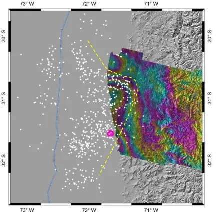
Figure 8. Map showing comparison between the aftershock distribution and the post-seismic deformation field. Pink point indicates Mw8.3 Mainshock, small white points mean aftershock (http://earthquake.usgs.gov, as of 11/10/2015),Blue dashed line shows the Chile trench,Yellow dashed line may be the projection of leading edge of the deductive plate tongue,a fringe stangards for 2.8cm displacement in LOS
The observation results that the post-seismic deformation includes uplift and subsidence areas along the Chile coast is probably related with the existing traverse fault that coordinates plate motion. This fault may expose on the surface, or hides beneath the ground (where there is a major river as seen on Google Earth). The presence of this traverse fault can result in different locking and slip characteristics along the subduction zone. South to this fault, the motion of the oceanic crust after the earthquake dominates the subducting slab, while the displacement opposite to the coseismic in the continent due to drag from the underlying oceanic plate. While north of this fault,
the post-seismic motion of the oceanic crust was not very intense, thus leading to post-seismic residual slip consistent with the coseismic deformation. This inference can also be confirmed by the relationship between the aftershock distribution and post-seismic deformation field (Figure8). Overall, the aftershocks are distributed along the nearly north-south trending subduction zone, but showing an arc-like protrusion toward east nearby 31°S, just coinciding the location with large post-seismic displacement. It means that there may exist a tongue-like slab here within the oceanic plate, which might have moved at a larger rate than ether side after the mainshock. It would have overcome many small barriers on the fault plane, and ruptured those patches that remained connective after the mainshock, leading to occurrence of lots of aftershocks. After the main shock, the dominant drag of the oceanic plate was likely only effective in a short time, afterwards the coseismic deformation continued to be dominant, thus the coseismic residual slip was observed. These inferences will be tested by more data and further research in the future.
7. CONCLUSIONS
Using the Sentinel-1A/IW InSAR data, we captured the coseismic deformation fields caused by the 2015 Chile Mw8.3 earthquake. It consists of dense concentric semi-circular fringes convex to east with a dominant subsidence motion in LOS direction, The maximum LOS subsidence reaches about 133cm near the coast. The inversed fault slip distribution constrained by the InSAR data revealed a concentrated fault rupture zone located in the shallow part above the hypocenter. The maximum fault slip is over 8m at a shallow depth above 9km, located in the northwest of the epicenter. The slip is gradually decreasing to the deep subsurface, but the depth at which the coseismic slip drops to zero is variable along rupture zone. Slip in the Chile trench is large and reaches about 8m. The maximum depth where slip can be ignored is nearly 50km under the surface. The mean rake angle from inversion is 116.4°, consistent with the thrust fault motion. The seismic moment magnitude is Mw8.27, consistent with focal mechanism solutions from seismic waves.
We also analyzed four post-seismic interferograms with different time spans. The results show that the post-seismic deformation is primarily distributed in a 65km-wide zone along the coast, with complex spatial and temporal variations. LOS uplift was prominent within 1-24 days after the mainshock, opposite to the coseismic deformation. Meanwhile a smaller area of subsidence appeared north to this uplift zone, resulting in relative displacement up to 11cm. Between them, there may exist an active fault. Within 24-48 days after the mainshock, the post-seismic deformation still occurred along the coast, but with remarkable changes in direction and magnitude. Overall, it was LOS subsidence, consistent with the coseismic, having smaller amplitude (less than 8cm), and tending to increase with time. Our analysis suggests that these features are due to that the underlying oceanic plate continued to dominate the seismic rupture plane at the early time after the mainshock, the drag of which resulted in the deformation opposite to the coseismic displacement. At the later time, as this drag became weak, the post-seismic residual slip was dominant on the rupture plane, thus appearing again the deformation consistent with the coseismic deformation.
Acknowledgements
work was supported by the National Natural Science Foundation of China (41374015, 41461164002) and National Key Laboratory of Earthquake Dynamics (LED2015A03,LED2013A02).
References
Delouis, B., et al., 2010. Slip distribution of the February 27, 2010 Mw = 8.8 Maule Earthquake, central Chile, from static and high‐rate GPS, InSAR, and broadband teleseismic data. Geophys. Res. Lett., 37, L17305.
Delouis, B., et al., 1997. The Mw = 8:0 Antofagasta (northern Chile) earthquake of 30 July, 1995: A precursor to the end of the large 1877 gap, Bull. Seismol. Soc. Am., 87, 427–445.
Delouis, B., Pardo M., Legrand D., and Monfret T., 2009. The Mw 7.7 Tocopilla earthquake of 14 November 2007 at the southern edge of the northern Chile seismic Gap: Rupture in the deep part of the coupled plate interface. Bull.Seismol.Soc.Am., 99,87–94.
Fred F. Pollitz, Ben Brooks, Xiaopeng Tong, et al., 2011. Coseismic slip distribution of the February 27, 2010 Mw 8.8 Maule, Chile earthquake. Geophys. Res. Lett., 38, L09309.
Jónsson, S., Zebker, H., Segall, P., et al., 2002. Fault slip distribution of the 1999 Mw7.1 Hector Mine, California, earthquake, estimated from satellite radar and GPS measurements. Bull. Seismol. Soc. Am., 92 (4), 1377–1389.
Mendoza, C., Hartzell S., and Monfret T., 1994. Wide‐band analysis of the 3 March 1985 central Chile earthquake: Overall source process and rupture history, Bull. Seismol. Soc. Am., 84, 269–283.
Pritchard, M. E., and Simons M., 2006. An aseismic slip pulse in northern Chile and along‐strike variations in seismogenic behaviour. J. Geophys. Res., 111, B08405.
Wang, R., Motagh, M., Walter, T.R., 2008. Inversion of slip distribution from coseismic deformation data by a sensitivity-based iterative fitting (SBIF) method. EGU General Assembly 2008, 10, EGU2008-A–07971.
Xiaopeng Tong, David Sandwell, Karen Luttrell, Benjamin Brooks, et al., 2010. The 2010 Maule, Chile earthquake: Downdip rupture limit revealed by space geodesy. Geophys. Res. Lett., 37, L24311.
Vigny C., Socquet A., Peyrat S., et al., 2011.The 2010 Mw 8.8 Maule Megathrust Earthquake of Central Chile, Monitored by GPS. Science, 332,1417—1421.
Marone C. J., Scholz C. H., and Bilham R., 1991.On the mechanics of earthquake afterslip. J.Geophys.Res., 96, 8441— 8452.