isprs archives XLI B4 557 2016

OPEN STREET MAP DATA AS SOURCE

FOR BUILT-UP AND URBAN AREAS ON GLOBAL SCALE

Thomas Brinkhoff

Institute for Applied Photogrammetry and Geoinformatics (IAPG), Jade University Wilhelmshaven/Oldenburg/Elsfleth Ofener Str. 16/19, D-26121 Oldenburg, Germany - thomas.brinkhoff@jade-hs.de

KEY WORDS: Built-up Areas, Urban Areas, Volunteered Geographic Information, OpenStreetMap, Spatial Data Processing

ABSTRACT:

Many types of applications require information about built-up areas and urban areas. Thus, there is a need for a global, vector-based, up-to-date, and free dataset of high resolution and accuracy. The OpenStreetMap (OSM) dataset fulfills those demands in principle. However, its focus is not land use or land cover. These observations lead to following questions: (1) Which OSM features can be used for computing built-up areas on global scale? (2) How can we derive built-up and urban areas on global scale in sufficient accuracy and performance by using standard software and hardware? (3) Is the quality of the result sufficient on global scale? In this paper, we investigate the first two questions in detail and give some insights into the third question.

1. INTRODUCTION

Many types of applications require information about built-up areas and – on larger scale – about urban areas. Prominent examples are standard street maps and topographical maps using such areas for visualization purposes (Nivala et al., 2008) as well as analyses about population development or land consumption (Esch et al., 2013).

For being widely used by desktop, web or mobile applications, the existence of a dataset is desirable that fulfills following requirements: (a) the dataset should be global, (b) the dataset should contain vector data (i.e., polygons), (c) resolution and accuracy should be in a range that is sufficient for most applications (10m or better), (d) the data should be up-to-date, and (e) the dataset should be provided as open data under a free license. At least requirement (b) needs some justification: In web mapping, SVG-based tiles replace more and more raster-based tiles because of performance and styling issues (Neumann, 2012). Furthermore, many applications work in different scales. Thus, a suitable generalization is important. Polygons allows a generalization by simplification, by selection, and by aggregation. The selection will be typically based on polygon areas (or similar measures). Therefore, the polygons in the dataset must be disjoint; otherwise, the selection criterion would be wrong. In other words, the generalization requires merging of overlapping, touching, or nearby areas.

The Corine Land Cover (CLC) database provides classified land cover data (e.g., continuous urban fabric, discontinuous urban fabric, industrial or commercial units) for the countries of the European Union in raster and vector format. The resolution of the data is 100m. The CLC database fulfills requirements (b) and (e), but not (a) and (c). The last update has been produced in 2012. The OpenStreetMap (OSM) dataset fulfills all five demands. However, its focus is not land use or land cover. Thus, the question for suitability arises. Previous work of several authors (see Section 2) indicates that the OSM dataset can be used for deriving land use and land cover information on regional scale or for well-digitized regions

Resulting questions are: (1) Which OSM features can be used for computing built-up areas on global scale? (2) How can we derive disjoint polygons for describing built-up areas and urban areas on global scale in sufficient accuracy and performance by using standard software and hardware? (3) Is the quality of the result sufficient on global scale? In the following, we will concentrate on the first two topics and give some insights into the third question.

The remainder of this text is organized as follows. Section 2 presents related work. The third section discusses the suitability of different OSM features for deriving built-up areas. Algorithmic and performance aspects are investigated in Section 4. Merging sets of polygons is among these topics. The fifth section is a preliminary evaluation of the results. The paper concludes with a short summary and an outlook to future work.

2. RELATED WORK

The extraction of built-up areas belongs to the field of land cover exploration for describing the physical coverage of land. For the derivation of urban areas not only the land cover (“urban form”) (Talen, 2003) but also urban function is considered (Smith & Crooks, 2010). In this work, however, we will compute urban areas purely from built-up areas.

If required on global scale, information about built-up areas will be typically derived from remote sensing data. Some few examples are the usage of Landsat 8 Operational Land Imager (OLI) data (Bhatti & Tripathi, 2014), the extraction from Advanced Spaceborne Thermal Emission and Reflection (ASTER) radiometer data (Miyazaki et al., 2014), and the use of Landsat TM/ETM+ images (Zhang et al., 2014). One recent effort in this field is the derivation of the so-called “urban footprint” from SAR imagery in the context of the TanDEM-X radar mission (Esch et al., 2013) (Marconcini et al., 2014).

Volunteers support the classification of remote sensing data in VGI (volunteered geographic information) projects. A prominent example is geo-wiki.org (Fritz et al., 2012).

Some studies have investigated deriving land use from OpenStreetMap data by using corresponding polygonal features (see also Section 3.2). However, this has been done in local scale, typically for one or several cities (Vaz & Jokar Arsanjani, 2015) (Jokar Arsanjani et al. 2015), for smaller regions (Dorn et al., 2015) or single countries (Estima & Painho, 2013). Estima & Painho (2013) also provides a detailed mapping between OSM feature classes and CLC classes.

The merging of large sets of overlapping polygons was not applied by any of the previously mentioned publications. The field of computational geometry has investigated this or related questions. Margalit & Knott (1989) presented a general approach for computing the union, intersection and difference between two polygons. Nievergelt & Preparata (1982) proposed a plane-sweep algorithm that determines intersecting regions. A modified version allows also determining the union of polygons. Žalik (2001) presented a plane-sweep approach for merging a set of polygons with a time complexity of O(k log k) where k is the total number of polygon vertices plus the number of touching edges among those polygons. In contrast to such work, we are not interested in designing a new algorithm with (theoretical) low computing cost, but in exploiting existing programming libraries for a fast and robust processing of large sets of polygons.

3. INFORMATION ABOUT BUILT-UP AREAS IN THE OPENSTREETMAP DATASET

3.1 Data Model of OpenStreetMap

OpenStreetMap provides features by a topological data model (OSM Wiki, 2016). Node elements describe points in the space by their latitude, longitude and identifier. Links are called “ways”. Way elements consist of an identifier and an ordered list of between 2 and 2,000 nodes. These nodes are referenced by using their identifier. Relation elements allow describing relationships between other elements. One important use is the representation of faces by multipolygons. In that case, a relation consists of a sequence of references to way elements that form the outer and inner rings of the multipolygon.

A feature is based on one of those three elements. Furthermore, it consists of a list of key-value pairs called “tags”. In principle, arbitrary keys and values can be added to features. The OSM community agrees on certain key-value combinations for the most commonly used tags. This (non-static) agreement acts as an informal standard.

Interested parties can download OSM datasets from different web sites. The data model is either straightly coded by using XML or corresponding binary formats or it is converted into other popular data formats like shapefiles. In the second case, a loss of information may occur.

3.2 Land Cover in OpenStreetMap

Different keys in the OSM data model are employed for land cover (OSM Wiki, 2016): The “landcover” key has the status of a proposal and is not widely used; only about 18,400 elements currently exist (OSM Taginfo, 2016). The “surface” key was originally created for describing the surface of way elements (e.g., cobblestone for roads). In addition, it indicates the surface type of larger areas as a secondary tag. The “natural” tag serves as land cover information for vegetation-, water- and landform-related features. Exemplary values are “wood”, “beach”, and

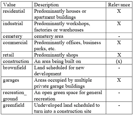
“valley”. The forth key related to land cover is “landuse”. It primarily describes agricultural areas (e.g., farmland), leisure areas (e.g., park), and built environment. The last category is relevant for determining built-up areas. Table 1 lists and describes the most often used values of this category.

Value Description Relevance

residential Predominantly houses or apartment buildings

X

industrial Predominantly workshops, factories or warehouses

X

cemetery cemetery area -

commercial Predominantly offices, business parks, etc.

X

retail Predominantly shops X

construction An area being built on (x) brownfield Land scheduled for new

development

-

garages Areas occupied by multiple private garage buildings

X

recreation_ ground

An open green space for general recreation

-

greenfield Undeveloped land scheduled to turn into a construction site

-

Table 1. The ten most often used values for the “landuse” key that belong to the “built environment” category (entries are

ordered by usage starting with the most often used value)

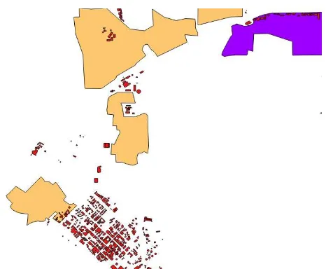
Figure 1. OSM built-up features for Oldenburg, Germany (light orange = “residential”, violet = “industrial”, brown =

“commercial”, red = “retail”, grey = “garages”)

Five of these values are obviously relevant for our purpose (indicated by an “X” in Table 1). Elements having a “landuse” tag with one of these five values will be called “OSM built-up features” in the following. Four values describe areas that are predominantly non-built-up or not built-up yet (indicated by a “-“). The relevance of the “construction” value is more difficult to assess because it depends of the stage of construction; it will not be used in the following but another decision would also be reasonable. There are currently 3.14 million residential features

and 1.19 million of other OSM built-up features in the OSM dataset.

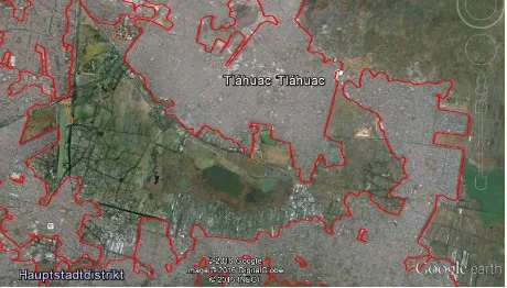
Figure 1 depicts the OSM built-up features for Oldenburg, Germany. The result looks very promising. However, this observation does not hold worldwide. For many countries, the coverage of the “landuse” features is poor. Figure 2 shows the result for Mexico City. In addition to the OSM built-up features, an urban-area layer is depicted in light green as reference. Obviously, most built-up areas are not covered. Furthermore, the accuracy of some OSM areas is rather low.

Figure 2. Built-up areas of Mexico City (OSM: light orange = “residential”, violet = “industrial”, brown = “commercial”, red = “retail”, grey = “garages”; urban-area layer: light green)

3.3 Buildings in OpenStreetMap

A further obvious source for built-up areas in the OSM dataset are buildings. Buildings are elements that have a tag with the key “building” (OSM Wiki, 2016). The value of the tag may describe the type of accommodation (e.g., “apartments”), of commercial use (e.g., “warehouse”), or of civic use (e.g., “church”). For about 83% of all buildings (OSM Taginfo, 2016), the value of the tag is purely “yes”. For our purpose, we can neglect the building typology. There are currently 181.4 million buildings stored in the OSM dataset.

Figure 3 shows buildings and OSM built-up features for a part of Darwin, Australia. It illustrates (a) that the OSM building dataset is not complete, (b) that the OSM building dataset partly covers areas not considered by OSM built-up features, and (c) that the buildings are much too detailed for describing built-up areas and even more urban areas. Thus, OSM buildings should be considered for deriving built-up and urban areas but need further processing (see Section 4).

Figure 3. OSM built-up features and buildings for a part of Darwin, Australia (light orange = “residential”, violet =

“industrial”, dark red = “buildings”)

3.4 Roads in OpenStreetMap

Roads are the third source of build-up areas. At first sight, this may be a surprising statement. However, special types of roads allow deriving information about the surroundings. For example, residential houses are typically built along residential roads. Roads in OpenStreetMap are (mostly way) elements with a “highway” tag (OSM Wiki, 2016). The corresponding value classifies the road. Table 2 lists and describes selected, often used values of the “highway” tag.

Value Description Relevance

residential Road in a residential area X service Access to a building, service

station, beach, campsite, industrial estate, business park, etc.

(x)

track Roads for agricultural and forestry use etc.

-

unclassified Public access road, non-residential

(X)

footway Designated footpaths, mainly/exclusively for pedestrians

(x)

tertiary A road linking small settlements - secondary A highway linking large towns - primary A highway linking large towns - cycleway Designated cycle ways (x) living_street Road with very low speed limits

and other pedestrian friendly traffic rules

X

motorway High capacity highways designed to safely carry fast motor traffic

-

pedestrian Roads mainly / exclusively for pedestrians

(x)

road Road with unknown classification

(x)

Table 2. Selected, often used values for the “highway” key (entries are ordered by usage starting with the most often used

value)

For two values (“residential” and “living_street”), we can rather definitely conclude that they are flanked by residential buildings. Tracks, tertiary roads, secondary roads, primary roads, and motorways are typically surrounded by no or only scattered houses. Thus, they are not of further relevance. Pedestrian paths, footways and cycle ways are often, but not always in residential or other built-up areas. Therefore, we are not considering them in the following. The description of “unclassified” clearly indicates that this key should be used outside of residential areas. However, the reality is different in many countries. Figure 4 shows unclassified highways in an area nearby Porto Alegre. The highways are clearly residential roads. Thus, the value “unclassified” has often (outside of Europe and North America) the meaning of “unknown” (which should be actually represented by “road”).

Figure 4. Roads with value “unclassified” for the key “highway” in an area nearby Porto Alegre, Brazil (satellite map

by Google Earth with images © Digital Globe)

There are currently 34.3 million roads in the OSM dataset classified as “residential” or as “living_street”. 9.0 million highways have “unclassified” as value and 0.3 million the classification “road”. Thus, neglecting “unclassified” highways would lead to a significant loss of information. Therefore, they will be included in the further processing; a corresponding algorithm will detect and filter most of the wrongly classified roads (see Section 4.3).

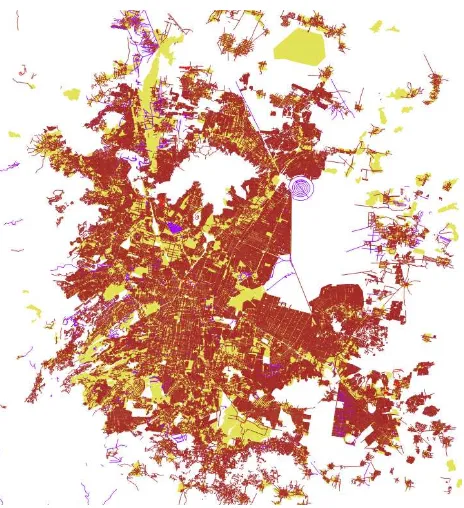
Figure 5 depicts residential roads, living streets and unclassified highways in the area of Mexico City. It illustrates (a) that the assumed coincidence between residential (and similar) roads and urban areas holds, (b) that the roads cover areas not considered by OSM built-up features (see also Figure 2), (c) that clusters of unclassified highways indicate built-up areas, and (d) that these clusters are disjoint to residential roads. Furthermore, some urban areas exist with a low density of residential roads or with no residential roads. The last observation will be picked up again in Section 5.

Roads as linear features are not suitable for describing built-up areas and urban areas in a straightforward way. As for buildings, a further processing is required.

Figure 5. Residential roads of Mexico City (OSM: dark red = “residential”, red = “living street”, violet = “unclassified”;

urban-area layer: light green)

4. DERIVING BUILT-UP AREAS AND URBAN AREAS FROM OPENSTREETMAP DATA

In the first three subsections, we present the processing of “landuse” features, of buildings, and of roads. The forth subsection deals with the combination of the results of the previous steps. Performance issues of subtasks are discussed in Section 4.5 and Section 4.6. The processing of large data sets is topic of the final subsection.

4.1 Processing of OSM Built-up Features

The goal of this processing phase is to compute a set of disjoint polygons describing built-up areas by using OSM built-up features (for definition see Section 3.2). Figure 6 gives an overview of the algorithm.

Figure 6. Algorithm 1 for processing OSM built-up features

Step 1 of the algorithm works obviously. The second step is necessary because some of the OSM built-up features are based on single way elements describing the outer ring of the corresponding area. In addition, multipolygons are disaggregated into polygons. As observed in Section 3.1, some OSM built-up features have a rather low accuracy. The accuracy can be determined by the quotient between the number of boundary points and the polygon area. If this quotient is lower than a given threshold, step 3 will eliminate

1. Read OSM features with „landuse” tag whose value in [“residential”, “industrial”, “commercial”, “retail”, “garages”] from input file.

2. Construct polygons.

3. Eliminate polygons with low accuracy. 4. Merge polygons with buffer distance x.

5. Reduce size of polygons by buffering with distance –x. 6. Generalize polygons.

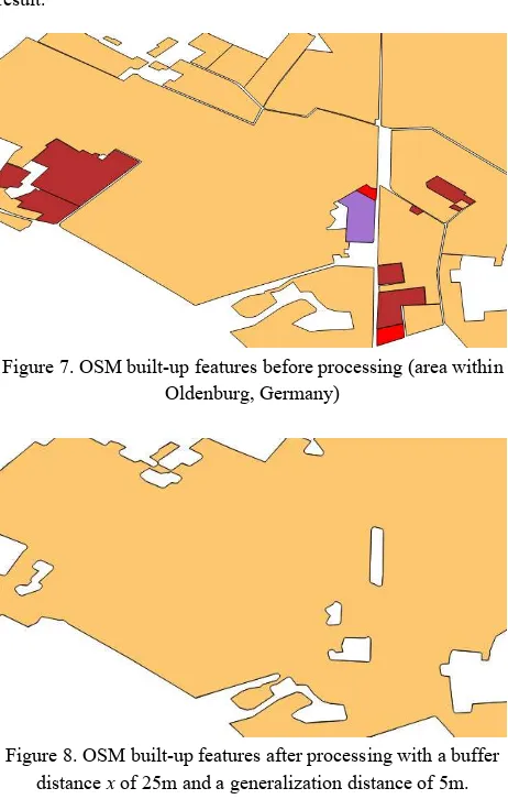
such a feature. As depicted in Figure 7, small gaps between the built-up features occur mostly caused by streets or small rivers. Furthermore, we are (in our use case) not interested in a differentiation of land-use classes. Thus, step 4 buffers all features by a small distance x and merges all overlapping polygons to single polygons. Algorithmic issues of this step are discussed in Section 4.5. The fifth step redeems the increase of extension by applying an inverse buffering with distance –x. Finally, the polygons are generalized. The generalization consists of eliminating small polygons, removing small holes and simplifying the boundaries depending on the required resolution. This step removes also dense sequences of points caused by the previous buffer operations. Figure 8 depicts the result.

Figure 7. OSM built-up features before processing (area within Oldenburg, Germany)

Figure 8. OSM built-up features after processing with a buffer distance x of 25m and a generalization distance of 5m.

4.2 Processing of OSM Buildings

The objective of this stage is to compute a set of disjoint polygons describing built-up areas by using OSM buildings. The proceeding is similar to the processing of OSM built-up features. Figure 9 gives an overview of the algorithm.

Figure 9. Algorithm 2 for processing OSM buildings

The quality of the footprints of the OSM buildings is sufficient so that an elimination of polygons with low accuracy is not necessary. However, the number of buildings is generally quite high. Therefore, step 3 deletes all buildings that intersect a polygon from the result of algorithm 1. Algorithmic issues of this step are discussed in Section 4.6. Again, step 4 buffers and merges features to disjoined polygons. Because of the gaps between buildings, the resulting polygons have many small holes. The fifth step removes them before reducing the size of the polygons by inverse buffering (step 6). Now, the absolute value of distance x is halved because it is not reasonable to align built-up areas exactly at the walls of buildings. The generalization step is the same as before. Figure 10 illustrates the input and the result of the algorithm.

Figure 10. OSM buildings (red: removed buildings intersecting resulting polygons of algorithm 1 [depicted in light orange]; green: remaining buildings) and the resulting built-up areas (in brown) computed with an initial buffer distance x of 25m and a

generalization distance of 5m (area of Darwin, Australia)

4.3 Processing of OSM Highways

The third stage computes built-up areas from OSM highways. Figure 11 presents the corresponding algorithm.

Figure 11. Algorithm 3 for processing OSM highways

The first steps filters the relevant OSM features; for Europe, North America and other areas with high digitalization quality “unclassified” highways may also be removed. With the same motivation as before, the algorithm reduces the highway geometries by excluding areas covered by OSM built-up features. Because of the longish form of roads, the difference is computed. Again, step 3 buffers and merges the features to disjoined polygons. However, the buffer distance y should be

1. Read OSM features with „highway” tag whose value in [“residential”, “living_street”, “unclassified”]

from input file.

2. If result of algorithm 1 exists, then compute difference of highways and polygons from that result.

3. Merge geometries with buffer distance y. 4. Remove small holes.

5. Reduce polygon size by buffering with distance –1.75·y. 6. Increase polygon size by buffering with distance 1.5·y. 7. Generalize polygons.

1. Read OSM buildings from input file. 2. Construct polygons.

3. If result of algorithm 1 exists, then delete the buildings that intersect a polygon from that result.

4. Merge polygons with buffer distance x. 5. Remove small holes.

6. Reduce size of polygons by buffering with distance –x/2. 7. Generalize polygons.

larger than in the two stages before. The distance must be sufficient to cover residential blocks between two parallel residential roads. In the example in Figure 12, this distance is 75m instead of 25m as in the examples in Figure 7 and Figure 10. Step 5 and 6 are performed for avoiding that single residential roads or wrongly classified single roads span a built-up area. Figure 12 illustrates this effect clearly.

Figure 12. OSM residential roads (red: removed road segments after computing the difference with the resulting polygons of algorithm 1 [depicted in light orange]; green: remaining roads)

and the resulting built-up areas (in brown) computed with an initial buffer distance y of 75m and a generalization distance of

5m (area of Darwin, Australia)

4.4 Combination of Results and Finalization

The outcomes of the previous three stages – as illustrated in Figure 13 – have to be combined for the desired result. Figure 14 drafts the proceeding.

Figure 13. Processed OSM built-up features (light orange), OSM buildings (red) and OSM highways (brown) for Darwin,

Australia

After storing all features in one layer, step 2 merges all overlapping polygons to single polygons. The buffer distance z depends on the desired result: For detailed built-up areas z can be 0, for rougher urban areas a higher distance is reasonable. The merge step leads to small holes that step 3 removes. The categorization in step 4 indicates an important potential of the resulting vector dataset: We can categorize the resulting

polygons by their geometric properties (e.g., by their area) and use this information by further applications (e.g., for a dynamic mapping in different scales). For computing urban areas, a further generalization is required. Figure 15 depicts the result.

Figure 14. Algorithm 4 for combination and finalization

Figure 15. Combined and generalized built-up areas for Darwin, Australia (buffer distance z = 15m)

4.5 Merge of Buffered Geometries

An important task of all previous algorithms is the merging of overlapping buffered geometries into a set of disjoint polygons. The simplest solution is to aggregate all geometries into a single geometry (i.e., a geometry collection), to buffer this geometry and to disaggregate the resulting multipolygon into single polygons (that are disjoint because the components of a multipolygon must be disjoint). For larger sets of geometries, this approach is not efficient (or breaks because of space limits or geometric inconsistencies).

For mid-size sets of geometries, the algorithm depicted in Figure 16 is applied. The quadtree is a MX-CIF Quadtree (Samet, 1990) implemented by JTS (JT, 2016). It allows storing and querying two-dimensional rectangles. Notice that step 4 does not test whether the geometries actually intersect. Thus, the result may include multipolygons. If only polygons are accepted in the result, step 7 must be applied. This is necessary for algorithm 4 before categorizing the polygons.

For large sets of highways or buildings, also this algorithm is too slow. Then, the data space is gridded and each geometry is assigned to exactly one grid cell using its centroid. For each grid cell, all of its geometries are merged by using algorithm 5. A further merging is not performed. Thus, the resulting (multi) polygons are not completely disjoint. As long as only algorithms 1 to 3 use the grid approach and algorithm 4 (which handles smaller sets of geometries) use algorithm 5, there is almost no impact on the final result.

1. Store the results of algorithms 1 to 3 in one layer. 2. Merge polygons with buffer distance z.

3. Remove small holes. 4. Categorize polygons.

5. (optional) Generalize polygons.

Figure 16. Algorithm 5 for buffering and merging sets of geometries

4.6 Intersection and Difference

Determining the intersecting polygons in step 3 of algorithm 2 and computing the difference between geometries in step 2 of algorithm 3 cannot be performed with linear cost. Both steps require determining the intersecting pairs of envelopes between two sets of geometries. In other words, a spatial intersection join is performed (Brinkhoff et al., 1993). Here, we use the MX-CIF Quadtree again with one set of geometries stored in the quadtree. The envelopes of the geometries of the other set serve as query rectangles.

4.7 Processing of Global OSM Data

For computing build-up areas or urban areas on global scale, the input dataset should be parceled into smaller tiles, e.g. into stripes of 1 or 2 degree width. A variant of algorithm 5 can combine two sets containing processed built-up areas. The main differences of this algorithm are: (a) all polygons of the first set are inserted into the quadtree at the beginning, (b) the algorithm iterates only over the polygons of the second set, and (c) all polygons of the second set, which intersect no polygon of set 1, also belong to the result set. If the overlap between the two sets is small, the algorithm is rather fast. A global OSM dataset can be completely processed (partitioning, stages 1 to 3, and combination) within few days on a single personal computer.

5. PRELIMINARY EVALUATION

As indicated by Figure 1, for some (well-digitized) countries (like Germany) the processing of OSM built-up features (i.e., the application of algorithm 1) is sufficient. Therefore, we restrict the further discussion of results to the example of Mexico City.

Figure 2 has shown that only few OSM built-up features exist for Mexico City. Figure 17 depicts the combined result for Mexico City using parameters as in the examples before together with a reference dataset. We can observe three significant differences indicated by blue numbers and ovals. The area (1) belongs to the Santa Lucia Airport, which is a mostly unbuilt area. Area (2) – as shown in Figure 18 by a screenshot from Google Earth – is also an unbuilt area. In these two cases, the computed build-up areas are more reliable than the reference dataset.

There are several areas not covered by the computed build-up areas in the oval labelled with 3 in Figure 17. Figure 19 from Google Earth shows that these areas are industrial zones. This shows an actual drawback of the presented approach: Industrial areas cannot be detected if they are not included in the OSM

built-up areas and if their buildings are not included in the OSM buildings.

Figure 17. Comparison of the computed built-up areas (red) with a reference layer (light green)

Figure 18. Evaluation of area (2) by Google Earth (with images © DigitalGlobe)

Figure 19. Evaluation of a part of area (3) by Google Earth (with images © DigitalGlobe)

1. Create empty quadtree q.

For all geometries g perform steps 2 to 5: 2. Buffer g with distance d.

3. Query q with Envelope(g).

4. For all query results: remove them from q and compute stepwise the union with g.

5. Store the result in q.

6. All geometries stored in q form the result. 7. Disaggregate multipolygons if required.

6. CONCLUSIONS

The paper has demonstrated that an extraction of build-up areas from the OSM dataset is feasible on global scale. The processing can be done within several days using standard hardware and software; the Java library JTS was used for geometry processing. First results look promising but need further investigation. The representation by disjoint polygons supports generalization and deriving urban areas.

Future work consists of a better support of industrial zones. Highways tagged as “service” are currently ignored. This tag may be used – together with a special arrangement of these roads – as indicator for built-up industrial areas.

A more extensive investigation of the parameterization of the algorithms and of the resulting quality of the built-up areas also belongs to future work. In (Esch et al., 2013), the publication of a global “urban footprint” with a resolution of 12m and of a public domain version downscaled to 50 to 75m are announced (and currently expected for mid-2016). We plan a systematic comparison with these datasets.

REFERENCES

Bhatti, S. S. & Tripathi, N. K., 2014. Built-up area extraction using Landsat 8 OLI imagery. GIScience & Remote Sensing, 51(4), pp. 445-467.

Brinkhoff, T., Kriegel, H.-P., Schneider, R., Seeger, B., 1993. Multi-Step Processing of Spatial Joins. Proceedings ACM

SIGMOD International Conference on Management of Data,

Minneapolis, MN, pp. 209-220.

Dorn, H., Törnros, T., Zipf, A., 2015. Quality Evaluation of VGI Using Authoritative Data – A Comparison with Land Use Data in Southern Germany. ISPRS International Journal of Geo-Information, 4(3), pp. 1657-1671.

Esch, T., Marconcini, M. et al., 2013. Urban Footprint Processor – Fully Automated Processing Chain Generating Settlement Masks From Global Data of the TanDEM-X Mission. IEEE Geoscience and Remote Sensing Letters, 10(6), pp. 1617-1621.

Estima, J. & Painho, M., 2013. Exploratory analysis of OpenStreetMap for land use classification. Proceedings 2nd

ACM SIGSPATIAL International Workshop on Crowdsourced and Volunteered Geographic Information, pp. 39-46.

Fritz, S., McCallum, I., Schill, C., Perger, C., See, L., Schepaschenko, D., Obersteiner, M., 2012. Geo-Wiki: An online platform for improving global land cover. Environmental Modelling & Software, 31, pp. 110-123.

Hagenauer, J. & Helbich, M., 2012. Mining urban land-use patterns from volunteered geographic information by means of genetic algorithms and artificial neural networks. International Journal of Geographical Information Science, 26(6), pp. 963-982.

Jokar Arsanjani, J., Mooney, P., Zipf, A., Schauss, A., 2015. Quality assessment of the contributed land use information from OpenStreetMap versus authoritative datasets. In: Jokar Arsanjani, J. et al. (eds.), OpenStreetMap in GIScience, Springer, pp. 37-58.

JTS, 2016. JTS Topology Suite,

https://sourceforge.net/projects/jts-topo-suite/ (05 April 2016)

Marconcini, M., Metz, A., Esch, T., Zeidler, J.: Global Urban Growth Monitoring by Means of SAR Data. Proceedings IEEE

International Geoscience and Remote Sensing Symposium,

Quebec, QC, pp. 1477-1480.

Margalit, A. & Knott, G. D., 1989. An algorithm for computing the union, intersection or difference of two polygons. Computers & Graphics, 13(2), pp. 167-183.

Miyazaki, H., Shao, X., Iwao, K., Shibasaki, R., 2014: Development of a Global Built-Up Area Map Using ASTER Satellite Images and Existing GIS Data. In: Weng, Q. (ed.), Global Urban Monitoring and Assessment through Earth Observation, CRC Press, pp. 121-142.

Neumann, A., 2012. Web Mapping and Web Cartography. In: Kresse, W. & Danko, D. (eds.), Springer Handbook of Geographic Information, Springer, pp. 567-587.

Nievergelt, J. & Preparata, F. P., 1982. Plane-sweep algorithms for intersecting geometric figures. Communications of the ACM, 25(10), pp. 739-747.

Nivala, A. M., Brewster, S., Sarjakoski, T. L., 2008. Usability evaluation of web mapping sites. The Cartographic Journal, 45(2), pp. 129-138.

OSM Taginfo, 2016: OpenStreetMap Taginfo,

https://taginfo.openstreetmap.org/ (05 April 2016)

OSM Wiki, 2016. OpenStreetMap Wiki,

https://wiki.openstreetmap.org/wiki/ (05 April 2016)

Samet, H., 1990. The Design and Analysis of Spatial Data Structures, Addison-Wesley, Reading, MA.

Smith, D. & Crooks, A., 2010. From Buildings to Cities: Techniques for the Multi-Scale Analysis of Urban Form and Function. UCL Working Papers Series, Paper 155.

Talen, E., 2003. Measuring urbanism: Issues in smart growth research. Journal of Urban Design, 8(3), pp. 195-215.

Vaz, E. & Jokar Arsanjani, J., 2015: Crowdsourced mapping of land use in urban dense environments: An assessment of Toronto. Canadian Geographer / Le Géographe canadien, 59(2), pp. 246-255.

Žalik, B., 2001. Merging a set of polygons. Computers & Graphics, 25(1), pp. 77-88.

Zhang, J., Li, P., Wang, J., 2014. Urban Built-Up Area Extraction from Landsat TM/ETM+ Images Using Spectral Information and Multivariate Texture. Remote Sensing, 6(8), pp. 7339-7359.