COMPARISON OF UNSUPERVISED VEGETATION CLASSIFICATION METHODS
FROM VHR IMAGES AFTER SHADOWS REMOVAL BY INNOVATIVE ALGORITHMS
Movia A., Beinat A. and Crosilla F.
Department of Civil Engineering and Architecture, via delle Scienze 206, University of Udine, Italy [email protected]
KEY WORDS: shadow removal, classification, VHR images, Procrustes methods, vegetation
ABSTRACT:
The recognition of vegetation by the analysis ofvery high resolution (VHR) aerial images provides meaningful information about environmental features; nevertheless, VHR images frequently contain shadows that generate significant problems for the classification of the image components and for the extraction of the needed information.
The aim of this research is to classify, from VHR aerial images, vegetation involved in the balance process of the environmental biochemical cycle, and to discriminate it with respect to urban and agricultural features. Three classification algorithms have been experimented in order to better recognize vegetation, and compared to NDVI index; unfortunately all these methods are conditioned by the presence of shadows on the images. Literature presents several algorithms to detect and remove shadows in the scene: most of them are based on the RGB to HSI transformations. In this work some of them have been implemented and compared with one based on RGB bands. Successively, in order to remove shadows and restore brightness on the images, some innovative algorithms, based on Procrustes theory, have been implemented and applied. Among these, we evaluate the capability of the so called “not-centered
oblique Procrustes” and “anisotropic Procrustes” methods to efficiently restore brightness with respect to a linear correlation correction based on the Cholesky decomposition.
Some experimental results obtained by different classification methods after shadows removal carried out with the innovative algorithms are presented and discussed.
1. INTRODUCTION
High resolution images like those acquired by UAV and satellite missions such as IKONOS or Quickbird, have increased remote sensing application fields, since they provide a greater detail than usual technologies (Arevalo et al., 2008). High resolution aerial images can support energy studies, for biomass estimation, water analysis , specifically for detecting pollution, environment and ecology investigations, for estimating urban sprawl and measurement of the climate change.
Classification of vegetation, in particular, is a key instrument for ecology and environmental management; in fact plants play an important role as component of ecosystems and they are involved in the regulation of different biogeochemical cycles like that of carbon (Xiao et al., 2004, Xie et al., 2008). For the purposes of extracting vegetation from images, literature commonly uses automatic classification procedures or specific spectral indexes in order to identify land cover data and discern vegetation in urban and rural areas (Xie et al., 2008). Classification methods indeed, recognize different surface types on the images and can automatically generate thematic maps, without the intervention of the user or with minimal actions of him. These techniques are based on spectral information of the pixels: each one is classified into a specific land cover class based on its reflectance. Two kinds of procedures, supervised and unsupervised methods, are commonly used for classifying images (Richards, 2013). Supervised classification is based on the idea that a user can orient the classification by assigning a specific class to a group of pixels, while the unsupervised classification is based on a software analysis of the image and the user provides only the number of the output classes. In the unsupervised classification the analyst plays no role in class attribution until the computations are completed. Pixels are allocated to a cluster through a minimum distance assignment rule and if a group of pixels is identified with a land cover class, all pixels of that cluster are consider to belong to that (Richards,
2013). This approach is usually used when training data for supervised classification are not obtainable, or are too expensive to acquire, or when the dataset presents high dimensions.
Specifically, literature presents several methods to achieve a correct unsupervised classification for detecting vegetation; among these Maximum Likelihood (Gromyko and Shevlakov, 2004), K-means (Thomas and Cathcart, 2008) and Self Organizing Map (Yuan et al., 2009) are some of the techniques more used in the last years.
An alternative to the unsupervised classification methods for the automatic detection of vegetation, is the calculation of a conventional spectral vegetation index: the most commonly used index is the Normalized Difference Vegetation Index (NDVI) (Saha et al., 2005, Xie et al.,2008). This index takes into account the near infrared band (IR band) and the red band (R band). NDVI values, by definition, range between -1 and +1, where high positive values indicate increasing green vegetation while negative values show non-vegetated surface features such as water, ice, snow, or clouds.
As already mentioned, VHR images provide much details about the scene; however they also introduce problems like cloud and cast shadows that generate big troubles in the classification of images and can bring to incorrect derived spectral information (Domenech and Mallet, 2014).
1.1 Shadow Detection
Several computer vision applications deal with shadow detection, in particular for the enhancement of photographic images (Xu et al., 2006) and video sequences (Prati et al., 2011).
The existing algorithms for shadow detection described in literature involve many user input parameters, but for the purpose of automation, i.e. for the aim of this work, priority is given to techniques that facilitate the automatic extraction of shadows from the scene.
Analyzing the state of the art of detection methods, literature categorizes the first step of shadow analysis -the detection one- into two classes (Arevalo et al., 2008): property- based and model-based methods. Adeline et al., (2013) later introduced two more categories: physics-based and machine learning methods.
The property based methods take into account the properties of shadows that can be gather from images and do not require any a priori information. These methods comprise techniques like histogram thresholding, invariant color models and object segmentation.
Otsu (1979) for the first time developed a method to identify shadow pixels from no shadow ones evaluating the gray-level of the images. In the same year Nagao et al. (1979) combined four bands of an aerial image in the following relation, for defining a shadow mask (SM):
SM= (1/6)*(2R+G+B+NIR) (1)
where NIR =Near Infrared Band R=Red band
G=Green band B=Blue band
Following this kind of approach, Dare (2005), Chen (2007) and Yamazaki (2009) used satellite panchromatic images to detect shadows by a thresholding method.
As previously mentioned, it is possible to detect shadows also by using invariant color models. Tsai and Lin (2006) converted RGB images into HSI (Hue- Saturation and Intensity), HSV (High- Saturation - Value), HCV (Hue- Chroma- Value) and YCbCr (SECAM color TV standard with luminance and two chrominance components) component spaces. The same authors (2006) also developed a spectral ratio between Hue and Intensity. Chung et al. (2009) improved the spectral ratio of Tsai and Lin (2006) and demonstrated that their method is more accurate compared to that of Tsai and Lin.
Model based methods can be divided in geometrical and physics-based ones. Geometrical methods need some a priori information like 3D geometry of the scene and illumination condition. Nakajima et al. (2002) and Zhan (2005), developed a first solution that takes into account Airborne Laser Scanning (ALS) data. From these data it is possible to derive the Digital Surface Model (DSM). Afterwards from DSM, high spatial resolution data, introducing sun azimuth and zenith, it is possible to calculate the location of shadows. Physical methods instead require information about material reflectance and an accurate knowledge on the environmental and atmospheric conditions of the scene. Finally, machine learning methods concern an unsupervised or supervised classification of the scene.
1.2 Shadow Restoration
As mentioned, in order to classify vegetation in a high resolution image it is necessary to eliminate or at list reduce shadows. Literature presents three main categories of shadow
correction methods: gamma correction, histogram matching and linear correlation (Sarabandi, 2004).
1.2.1 Gamma Correction. Gamma correction methods consider shadows as an inconvenient that disturbs brightness images in few digital numbers. To solve the problem, a new digital number called DN recovered is calculated as follows.
(2)
In the case of 11-bit image, the equation is solved as follows:
(3)
The value should be estimated for every image using local sampling data and it is specific only for the class of land use for which it is computed. To calculate coefficient, the mean value of shadow pixels and the mean value of neighboring
Using the least squares error criterion, the linear function for restoring shadow pixels is:
μshadow+μn n (4)
is considered the mean value; is the standard deviation of the shadow/non shadow region (Sarabandi, 2004).
Chang and Tsay (2010) modified this equation introducing previous shaded pixel value. The equation becames:
2. METHOD APPLIED
Image classification is usually performed by traditional unsupervised methods like K-means and Self Organised Maps (SOM). These approaches are often used in thematic mapping from imagery, including vegetation cover identification. In the unsupervised classification methods the image is used to generate clusters and all pixels can be allocated to one of the clusters through a minimum distance criterium. Because of the presence of shadows in the scene, automatic classification methods cannot give good results and alternative methods like the spectral indexes for detecting vegetation are used instead. Spectral vegetation index evaluation is affected by the presence of shadows in the scene, so the authors considered necessary shadow detection and removal before applying the classification process.
2.1 Classification methods
In this paper it was decided to elaborate unsupervised classifications because of their automatic approach and because no land cover data at a suitable level of detail was available.
Moreover, for technical choice, authors used only the visible band-red, green, blue- for the clustering step due to the fact that Infrared band in VHR images is rarely provided. At first, a classification of the original image was performed. Authors considered only unsupervised techniques like K-means and Self Organizing Map implemented in Matlab and Maximum Likelihood implemented in Grass.
In remote sensing literature, Maximum Likelihood is commonly considered a supervised classification method. A specific utilization of this technique in Grass software can be associated to an unsupervised classification, processing first the i.cluster algorithm and then the i.maxlik one. In this way classification is based on the spectral signature generated by i.cluster and then refined by i.maxlik (Neteler and Mitasova, 2008).
The K-means clustering algorithm implemented in Matlab was used to partition the image in clusters and to produce a classification map. Square Euclidean distance measure was used in Matlab for cluster assignment.
Finally a Self-Organizing Maps classification was performed. The procedure considers the detection of five classes for the study area and the results cannot be considered suitable for the presence of shadows in the scene.
To test the results of the classification methods, thanks to the availability of the IR band for the dataset analyzed, the NDVI was calculated as follows:
-
(6)
2.2 Shadow Detection
For detecting shadows the spectral ratioing techniques developed by Tsai and Lin (2006) and that developed by Domenech and Mallet (2014) were performed. In the following step Otsu's method (Otsu, 1979) was applied for automatic determining of the optimal threshold to delineate shadows from no shadows regions.
The indexes considered and compared were those develop by Tsai and Lin (2006) and derived from the transformation of applied for every index map calculated. As a consequence, a Boolean shadow mask of the shadow region was obtained pixels identified correctly as shadow; FN (false negative) were the total number of true shadow pixels identified like goodness were evaluated: PA (Producer's Accuracy), CA (Consumer's Accuracy) and the OA (Overall Accuracy) defined in the following equations:
(12)
(13)
(14)
For completeness, another index the specificity (SP) proposed by Kanji (1999) was evaluated.
(15)
2.3 Shadow Restoration
Several shadow restoration methods are proposed in literature but they don't give a real solution for the compensation of shadows. Authors present a further approach to restore brightness in shadow pixels.
involved. Due to the large variety of image characteristics (exposure, contrast, saturation etc.) the conversion algorithm and its parameters must be chosen properly. Assuming an arbitrary transformation model, its coefficients can be locally computed, image by image, on the basis of a set of corresponding features, whose RGB pixel coordinates are known in shadow and light conditions.
Said L (light) the n×3 matrix formed by the RGB components of the n pixels in light, and S (shadow) the n×3 matrix of the corresponding n pixels in shadow, we assume the existence of a generic transformation T(n× n), for which:
(16)
Lorenzi et al. (2012) proposed the following relationship: (17)
where R is directly computed by way of the Cholesky decomposition of the covariance matrices of S and L, g is a translation vector and 1 is a unitary 1-by-n vector. Said CSS the covariance matrix of S, and CLL that of L, the Cholesky decomposition gives CSS=SCTSC and CLL=SLTSL, where SC and SL are both upper triangular matrices. It follows that: R=SLT(SCT)-1, and g=mean(L)T-Rmean(S)T. In this equation, R has no specific properties, while g (translation) can be interpreted as a general increment of every RGB components. To evaluate further conversion alternatives, having an eventual physical interpretation, the authors implemented and tested other transformation models, all derived from the Procrustes analysis. The algorithms considered are: the orthogonal Procrustes (OP), the extended orthogonal Procrustes (EOP), the oblique Procrustes without centering (ObP), the oblique Procrustes with centering (ObPC), and the extended anisotropic orthogonal Procrustes (EAOP) (Gower and Dijksterhius, 2004). The orthogonal Procrustes model is similar to the Cholesky's one: (18)
but here R is ortoghonal, that is R RT=RT R=I, where I is the identity matrix. R is computed in direct way as R=V WT, where V and W, in turn, are the eigenvector matrices of the Singular Value Decomposition of the matrix product of the original S and L: n (19)
and n n . The extended orthogonal Procrustes model is an extension of the previous one in which a global scale factor c is introduced: (20)
The transformation matrix R is computed by the same SVD of the matrix product of S and L, but here the scale factor c and the translation g are respectively – n and n n . The oblique Procrustes without centering is a straightforward transformation: (21)
Where R is directly computed as: Similar form has the algorithm of the oblique Procrustes with centering. Here, L and S are first centered: – n and – n then R is computed in similar way: . The relationship between shadow and light in the ObPC model becomes: n (22)
Last, the extended anisotropic orthogonal Procrustes, although not strictly a direct solution, has nevertheless a fast converging iterative computation (Garro et al., 2012). Respect to the EOP case, in which a global scale factor affects all the components of the color space, here an independent scale factor is applied to each RGB component. The RGB color rotation matrix R is still orthogonal. After having initialized the scale factors vector as D = [1 1 1], the following quantities: – n (23)
(24)
(25)
– (26)
where ./ represents the element-wise division, were repeatedly computed until convergence. The resulting transformation is: (27)
and n, where n, number of pixels, is given by n = 1 1T. (Fusiello et al., 2013).
The preliminary tests carried out, let us to select and compare for our goals the Cholesky, ObP and EAOP methods. Due to the limited space, the implementation of the analytical models for shadow removal, and an extended report on the experiments performed will be discussed in a separate paper.
3. DISCUSSION AND RESULTS
To evaluate the performance of the algorithm developed, a test dataset of Tavagnacco, a municipality in Friuli Venezia Giulia (Italy) has been firstly selected. The image of the area, dated December 2011, has a size of 20M pixel and a pixel resolution of 9 cm.
The scene is dominated by the presence of green areas and is contaminated by different types of long shadows, covering about 20% of the surface.
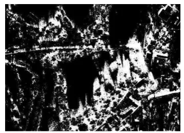
Figure 1: Original image classificated respectively with Maximum Likelihood (ML), K-Means (KM) and Self
Organized Map(SOM)
Results of the three methods showed that a large portion of pixels were misclassified due to the presence of shadows in the scene; the images reported before (figure 1) underline this.
In addition classifiers were not in accordance in the detection of vegetation.
The result of the NDVI index, reported in figure 2 underlines the fact that the presence of shadows compromised again the detection of vegetation.
Figure 2: Elaboration of the NDVI index
As already said shadow removal is a mandatory step before performing any kind of classification.
3.1 Shadow detection
Table 1 summarizes the accordance of the different shadow detection indexes with respect to the real shadow mask. Results underline that WBI and NSDVI indexes better identified shadow pixels and no shadow ones, with the WBI (figure 3) having an overall accuracy (OA) slightly better than NSDVI.
WBI NSDVI YCr HI HV
FP 3.54 2.51 22.74 36.10 33.80 FN 10.79 13.31 0.64 0.41 0.43 TP 18.17 15.64 28.32 28.55 28.52 TN 67.51 68.53 48.30 34.95 37.25 PA 62.74 54.02 97.80 98.60 98.51 CA 83.71 86.16 55.46 44.16 45.77 OA 85.68 84.17 76.62 63.49 65.77 SP 95.02 96.46 67.99 49.19 52.43
Table 1: Comparison of shadow detection methods
So this index elaborated by Domenech et Mallet (2014) can be used as a good mask to evidence shadows in the image.
Figure 3: Shadows mask calculated with the WBI index
3.2 Shadow restoration
Automatic shadow removal in a complex scene constitutes a challenging problem. For all the algorithms described the critical step is the correct identification of the corresponding set of pixels, in shadow and light conditions, to compose the matrices S and L respectively. In theory, this task would be performed locally, matching surfaces of the same nature (i.e. vegetation vs. vegetation, asphalt vs. asphalt, bare soil vs. bare soil etc.). At this stage of the research we adopted a global approach. We considered simultaneously all the pixels in shadow, and all the pixels in light on the image. Both lists were sorted on the basis of their panchromatic intensity. Then the largest dataset was under-sampled in order to obtain S and L of the same size. Finally, de-shadowing algorithms were applied.
Figure 4: Original image and image after deshadowing approaches. In order: EAOP, ObP and Cholesky
deshadowing methods
To this aim the authors used the EAOP, ObP and Cholesky methods, described before, that provided better performances in specific tests for the reconstruction of shadows.
The considered algorithms recreated an image with a residual amount of shadows, as reported in figure 4.
3.3 De-shadowed Map Classification
When the process of shadow removal was completed it was necessary to reclassify the images to compare the results between the three classification methods adopted. The images reported below significantly describe an enhancement of the classification after performing a shadow restoration.
The unsupervised classifications performed returns five classes that would be correspond to pavement roads, roofs, trees, grass and bare soil.
Figure 5: Reclassification of reconstructed image with Anisotropic Procrustes method. In order ML, KM, SOM
classifier
Figure 6: Reclassification of reconstructed image with not centered oblique Procrustes method. In order ML, KM,
SOM classifier
Figure 7: Reclassification of reconstructed image with Cholesky method. In order ML, KM, SOM classifier
From table 2 it is clear that classification depends from the type of classifier used and not from the shadow removal methodology.
Anisotropic Procrustes % of agreement
ML/SOM 39.35
KM/SOM 27.81
ML/KM 57.21
Cholesky % of agreement
ML/KM 55.28
KM/SOM 63.80
ML/SOM 57.98
Not- centered oblique Procrustes % of agreement
ML/SOM 34.69
ML/KM 58.42
KM/SOM 63.00
Table 2: Agreement between classifier results relative to different deshadowing methods
Moreover table 2 shows that the maximum likelihood classication is the more robust because it is in accordance with all shadow removal methods.
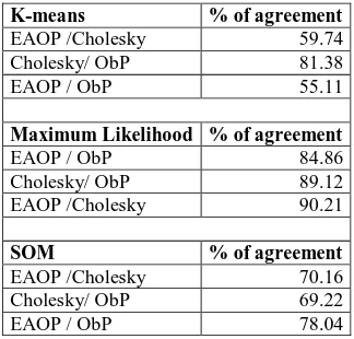
K-means % of agreement
EAOP /Cholesky 59.74
Cholesky/ ObP 81.38
EAOP / ObP 55.11
Maximum Likelihood % of agreement
EAOP / ObP 84.86
Cholesky/ ObP 89.12
EAOP /Cholesky 90.21
SOM % of agreement
EAOP /Cholesky 70.16
Cholesky/ ObP 69.22
EAOP / ObP 78.04
K-means classifier instead gives different results based on the shadow removal technique.
With the same shadow removal method instead, results of the images classifiers are different as demonstrated in table 3.
4. CONCLUSIONS
This paper covered a large number of topics in vegetation classification using high resolution imagery. After carrying out the state of this particular field of research the most common classifiers were applied to the original image to detect vegetation. Experiments show that the presence of shadows in the image cause a significant loss of radiometric information and produce wide and significant classification errors. It is undoubtedly that it is necessary to remove shadows for the enhancement of the results.
Removing shadows is a key step for an efficient detection of vegetation.
Furthermore, because of the radiometric limitations of the RGB channels, classification methods would be improved considering spatial information like context and texture. In a successive paper authors will present the results derived from the use of these new parameters extracted from RGB images associated with geometrical information obtained from ALS surveys.
REFERENCES
Adeline K.R.M., Chen M., Briottet X., Pang S.K. and Paparoditis N., 2013. Shadow detection in very high spatial resolution aerial images: A comparative study. ISPRS Journal of Photogrammetry and Remote Sensing 80 (2013) 21-38.
Arevalo V., Gonzales J., Ambrosio G., 2008. Shadow detection in colour high-resolution satellite images. International Journal of Remote Sensing. Vol.29, No. 7, 10 April 2008, 1945-1963.
Chang C. and Tsay J., 2010. Shadow Detection and Information Recovery in Aerial Images. In Proceedings of the 31st Asian Conference on Remote Sensing 2010.
Chen Y., Wen D., Jing L. and Shi P., 2007. Shadow information recovery in urban areas from very high resolution satellite imagery International Journal of Remote Sensing, 28:15, 3249-3254.
Chung K., Lin Y. andHuang Y., 2009. Efficient shadow detection of color aerial images based on successive thresholding scheme. IEEE transaction on Geoscience and Remote Sensing 47 (2) 671-682.
Dare P., 2005. Shadow analysis in high-resolution satellite imagery of urban areas. Photogrammetric Engineering and Remote Sensing, 71, pp. 169–177.
Domenech E. and Mallet C., 2014. Change Detection in High resolution land use/land cover geodatabases (a t object level). EuroSDR official publication No.64. April 2014.
Finlayson G.D.,Hordley, S.D., Cheng Lu, Drew, M.S., 2006. On the Removal of Shadows From Images. IEEE Transactions on Pattern Analysis and Machine Intelligence 28 (1), 59-68.
Fusiello A, Maset E., Crosilla F., 2013. Reliable exterior orientation by a robust anisotropic orthogonal Procrustes Algorithm. Int. Arch. of Photogrammetry, Remote Sensing and Spatial Information Sciences, vol. XL-5/W1, pp. 81-87.
Garro V., Crosilla F., Fusiello A., 2012. Solving the PnP Problem with Anisotropic Orthogonal Procrustes Analysis. In 3dimpvt, pag 262-269.
Gower J.C. and Dijksterhius G.B., 2004. Procrustes problems. Oxford University press 2004.
Gromyko M. and Shevlakov A., 2004. Classification Analysis of LANDSAT Images of Mixed Coniferous and Deciduous Riparian Forest in Nature Conservation Zone Using GRASS/PostGIS Link. Proceedings of the FOSS/GRASS
Users Conference − Bangkok, Thailand, 12−14 September
2004.
Kanji G.K., 1999. 100 Statistical Tests (Thousand Oaks, CA: SAGE).
Lorenzi L. Melgani F. and Mercher G., 2012. A Complete Processing Chain for Shadow Detection and Reconstruction in VHR Images. IEEE Transaction on Geoscience and Remote Sensing, Vol. 50, No. 9, September 2012.
Ma H., Qin Q., and Shen X., 2008. Shadow segmentation and compensation in high resolution satellite images. Geoscience and Remote Sensing Symposium, 2008. IGARSS 2008. IEEE International. Vol. 2. IEEE, 2008.
Nakajma T., Tao G. and Yasuoka Y., 2002. Simulated recovery of information in shadow area s on IKONOS image by combining ALS data. Proceedings of Asian Conference on Remote Sensing (ACRS).
Neteler M. and Mitasova H., 2008. Open Source GIS: A GRASS GIS Approach. Third Edition. The International Series in Engineering and Computer Science: Volume 773. 406 pages, 80 illus., Springer, New York. ISBN: 038735767X | ISBN-13: 978-0-387-35767-6 eBook e-ISBN-13: 978-0-387-68574-8.Published 1st Nov. 2007.
Otsu N., 1979. A threshold selection method from gray level histograms. IEEE Transaction on Systems, Man, Cybernetics 9 (1), 62-66.
Prati A., Mikic I.,Trivedi M.M. and Cucchiara R., 2003. Detecting Moving Shadows: Formulation, Algorithms and Evaluation. IEEE Trans. Pattern Analysis and Machine Intelligence, vol. 25, no. 7, pp. 918-923, July 2003.
Richards J.A., 2013. Remote Sensing Digital Image Analysis. An Introduction. Fifth Edition. Springer.
Saha A.K., Arora R.K., Csaplovics E. and Gupta R.P., 2005. Land Cover Classification Using IRS LISS III Image and DEM in a Rugged Terrain: A Case Study in Himalayas. Geocarto International, Vol. 20, No. 2, June 2005.
Sarabandi P., Yamazaki F., Matsuoka M., Kiremidjian A.,2004. Shadow detection and radiometric restoration in satellite high resolution images. IEEE IGARSS. Sep (2004), vol. 6, pp. 3744-3747.
Thomas A.M. and Cathcart J.M., 2008. Adaptive Spatial Sampling Schemes for the Detection of Minefields in Hyperspectral Imagery. in Proc. of SPIE Detection and Sensing of Mines, Explosive Objects, and Obscured Targets XIII 6953(28) (2008).
Tsai I-C. and Lin C.H., 2006. A comparative Study of Shadow Compensation of Color Aerial Images in Invariant Color Models. IEEE Transaction on Geoscience and Remote Sensing, Vol. 44, No. 6, June 2006.
using satellite images and climate data. Remote Sens Environ 91:256–70.
Xie Y., Sha Z., Yu M., 2008. Remote sensing imagery in vegetation mapping: a review.J Plant Ecol (2008) 1 (1): 9-23 doi:10.1093/jpe/rtm005.
Xu L., Qi F., Jiang R., Hao Y., Wu G. and Xu L., 2006. Shadow detection and removal in real images: A survey. Technical report, Shangai JiaoTong University, PR China.
Yamazaki F., Liu W. and Takasaki M., 2009. Characteristics of shadow and removal of its effects for remote sensing
imagery. In: Proc. International Geoscience and Remote Sensing Symposium, IGARSS, Cape Town, South Africa, 12 - 17 July, 4, pp 426-429.
Yuan H., Shi C.F. and Xiao S., 2009. An Automated Artificial Neural Network System for Land Use/Land Cover Classification from Landsat TM Imagery. Remote Sens. 2009, 1, 243-265; doi:10.3390/rs1030243.