3D LAND COVER CLASSIFICATION BASED ON MULTISPECTRAL LIDAR
POINT CLOUDS
Xiaoliang ZOU a, b, c, Guihua ZHAO c, Jonathan LI b, Yuanxi YANG a, c, Yong FANG a, c, *
a State Key Laboratory of Geo-Information Engineering, Xi’an, China 710054 – (zhz200271, yuanxi_yang)@163.com b Department of Geography and Environmental Management, Faculty of Environment, University of Waterloo, Waterloo, ON,
Canada N2L 3G1 – (x26zou, junli)@uwaterloo.ca
c Xi’an Institute of Surveying and Mapping, Xi’an, China 710054 – [email protected]
Commission I, ICWG I / VA
KEY WORDS: Multispectral Lidar, OBIA, Intensity Imagery, Multi-resolution Segmentation, Classification, Accuracy Assessment, 3D Land Cover Classification
ABSTRACT:
Multispectral Lidar System can emit simultaneous laser pulses at the different wavelengths. The reflected multispectral energy is captured through a receiver of the sensor, and the return signal together with the position and orientation information of sensor is recorded. These recorded data are solved with GNSS/IMU data for further post-processing, forming high density multispectral 3D point clouds. As the first commercial multispectral airborne Lidar sensor, Optech Titan system is capable of collecting point clouds data from all three channels at 532nm visible (Green), at 1064 nm near infrared (NIR) and at 1550nm intermediate infrared (IR). It has become a new source of data for 3D land cover classification. The paper presents an Object Based Image Analysis (OBIA) approach to only use multispectral Lidar point clouds datasets for 3D land cover classification. The approach consists of three steps. Firstly, multispectral intensity images are segmented into image objects on the basis of multi-resolution segmentation integrating different scale parameters. Secondly, intensity objects are classified into nine categories by using the customized features of classification indexes and a combination the multispectral reflectance with the vertical distribution of object features. Finally, accuracy assessment is conducted via comparing random reference samples points from google imagery tiles with the classification results. The classification results show higher overall accuracy for most of the land cover types. Over 90% of overall accuracy is achieved via using multispectral Lidar point clouds for 3D land cover classification.
1. INTRODUCTION
Most commercial airborne laser scanning systems are commonly monochromatic systems or dual-wavelength sensors recording either discrete echo or the full waveform of the reflected laser beams. Many researchers employ Lidar systems for vegetation analysis, bathymetry, topography and land cover classification. Airborne laser scanners have proved efficiency to retrieve fundamental forest parameters such as stand mean height, vertical structure, timber volumes, leaf area index, canopy closure, and above ground biomass. Valerie U. et al. (2011) presented an overview of the specific features of discrete return airborne Lidar technology relevant to 3D vegetation mapping application. Advanced discrete return sensors ALTM-Orion could produce data of enhanced quality, which could represent complex structures of vegetation targets at the level of details. Doneus et al. (2015) presented a compilation of recent airborne laser bathymetry scanning systems for documentation of submerged archaeological sites in shallow water. The SHOALS system (Irish and Lillycrop, 1999) employs Lidar technology to remotely measure bathymetry and topography in the coastal zone. It is an airborne Lidar bathymeter to use a scanning, pulsed, infrared (1064 nm) and blue-green (532 nm) laser sensor to measure the water surface and the penetration of the water surface to a certain depth. Leica AHAB HawkEye Lidar III system captures full waveform Lidar data from two bathymetric channels (10 kHz deep and 35 kHz shadow, 532nm) and one 500 kHz (1064nm) topographic channel. The Leica sensor scans with three channels but only in two wavelengths. It can collect totally
* Corresponding author
seamless data from land, the coastal zone and the seafloor down to a certain depth (Leica HawkEye III, 2015). Wang et al. (2014) proposed a dual-wavelength LiDAR system by integrating an Optech ALTM Pegasus HD400 (1064 nm) and a Riegl LMSQ680i (1550 nm) to combine surveys for a classification study of land cover. Based on the features of Lidar data such as dual-wavelength amplitude, echo width and surface height, a support vector machine was used to classify six types of suburban land cover: roads and gravel, bare soil, low vegetation, high vegetation, roofs, and water bodies. Results showed that using dual-wavelength LiDAR-derived information could compensate for the limitations of using single-wavelength LiDAR information when classifying land cover.
Teledyne Optech Inc. released the world’s first commercially multispectral airborne Lidar system Optech Titan on 24 November 2014 (Michael R. Sitar, 2015). Multispectral Lidar become a promising research domain that has attracted the interest of the scientific community and research groups. Optech Titan system can not only significantly improve existing application results, but also enable new vertical applications especially in high density topographic surveying, seamless shallow water bathymetry, and vegetative classification. Bakuła Krzysztof (2015) presented a multispectral Optech Titan system with the possibility of data including the analysis of digital elevation models accuracy and data density in three spectral bands, and discussed the possibility of the generation of colour composites using orthoimages of laser intensity reflectance and The International Archives of the Photogrammetry, Remote Sensing and Spatial Information Sciences, Volume XLI-B1, 2016
its classification capabilities using data from multispectral laser scanning for land cover mapping. As a result of the study, the high relative accuracy of Titan system in three spectral bands was proven. The mean differences between digital terrain models (DTMs) were less than 0.03 m. The data density analysis showed the influence of the laser wavelength. The point clouds had average densities of 25, 23 and 20 points per square metre respectively for green, near-infrared and shortwave-infrared lasers. Wichmann V. et al. (2015) presented an explorative analysis of the first multispectral airborne Lidar Titian ALTM collected data with focus on class specific spectral signatures. Spectral patterns were used for a classification approach, which was evaluated in comparison to a manual reference classification. They showed that this first flight data set was suitable for conventional geometrical classification and mapping procedures. Ahmed Shaker (2015) used multispectral Lidar data collected by Optech Titan system to assessment analysis for land cover classification results in two study areas in the city of Oshawa, ON, Canada. The first study area on the north of Oshawa was about 550m x 380m containing various types of land cover classes. Maximum likelihood classifier was used to classify the intensity data of each channel separately, combined three intensity bands, and a DSM band with three channels. Overall classification accuracy on Channel 1, 2, 3 separately was equal to 38%, 46% and 52.5%. Combined classification results of Channels 1, 2 and 3 intensity data, overall classification accuracy was 69%. A digital surface model (DSM) is added as an additional band to the combined three intensity bands, and overall classification accuracy reached 78%. The second study area on the south of Oshawa is flat urban area. By using object oriented classification method and normalized DSM with combined three intensity bands, the best overall accuracy reaches 94% for classification results.
Within this study, we also use a multispectral Lidar dataset captured by Optech Titian system for 3D land cover classification. The paper presented an approach to use directly three intensity images data with OBIA approach and the 3D properties of point clouds for classification, and to assess the validity of the 3D classification results.
2. OPTECH TITAN LIDAR SYSTEM
Multispectral Lidar Optech Titan system has a high-productivity sensor with an efficient and comprehensive workflow. Titan sensors consist of Optech multispectral laser scanning sensor, high-resolution QA 4-band aerial digital camera (CS-6500), position and orientation system (POSAV AP50), inertial measurement unit (IMU-46), storage and control unit. The Titan workflow includes an Optech flight management system (Optech FMS) and the industry-leading Lidar processing suite for automatic sensor calibration and project accuracy quantification (Titan Brochure and Specifications, 2015). Optech Titan system can emit simultaneous laser pulses at three different wavelengths. The reflected multispectral energy is captured through a receiver of the sensor, and the return signal together with the position and orientation information of sensor is recorded. These recorded data are solved with GNSS/IMU data for further post-processing, forming high density multispectral point clouds.
Optech Titan system works with three independent active channels at the wavelengths of 1550 nm (C1) in intermediate infrared band (IR), 1064nm (C2) in near infrared band (NIR) and 532 nm (C3) in visible green band. Each beam has a 300 kHz effective sampling rate for a combined ground sampling rate of 900 kHz. The repetition rate for all three channels can be programmable between 50 kHz to 300 kHz or a maximum total
of 900 kHz. Laser pulses of the three channels are sent to the same oscillating mirror with individual deflecting angles for each channel. This leads to separate optical light paths for each channel: 1550 nm (C1) 3.5° forward looking, 1064 nm (C2) 0° nadir looking, and 532 nm (C3) 7° forward looking. The scan angle (FOV) can be programmable between 0° to 60° or a maximum angle 60°. The sensor is capable of providing discrete point clouds data or full waveform record data at all three bands, and the receiver sensor is also capable to receive up to 4 returns with 4 - 12 bit intensity returns and waveform capture is 12-bit 1GS/sec. All three channels can operate at between 300 and 2000 meter AGL for topographic measurement, and the bathymetric C3 channel operates at 300-600 meter AGL for bathymetry. The high-resolution C3 channel ensures high density point clouds for shallow water mapping application. The discrete measurement method is more efficient than full waveform capture in seamless land/water measurement.
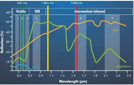
Titan system provides three independent point clouds data, one for each channel. Point clouds distribution is controlled using a fully-programmable scanner for significant point density increases at lesser FOVs. Point density can be greater than 45 points/m2 for topographic survey, and greater than 15 points/m2 for bathymetry. The horizontal specification accuracy is 1/7500 of altitude AGL and elevation accuracy is 5-10cm (Titan Brochure and Specifications, 2015). Figure 1 shows Lidar wavelength sensitivities for a broad spectrum of application, which is a relationship between wavelengths and reflectance properties of objects. Water is strongly penetrated in green spectrum. The laser of NIR and IR spectrums are completely absorbed by water bodies. Vegetation is strongly reflective in NIR spectrum, and slightly reflective in visible green spectrum. Soil is best reflective in intermediate infrared.
Figure 1. Lidar wavelength sensitivities for a broad spectrum of application (Titan Brochure and Specifications, 2015)
Optech Titan system is the first commercial multispectral active imaging sensor that enables a broad spectrum of application capability in a single sensor design. Titan system can not only provide for the possibility of surveying 3D data but also obtain spectral information about scanned objects in independent channels. By incorporating multiple wavelengths, it is capable of performing high density topographic mapping, shallow water bathymetry, vegetation mapping and 3D land classification.
3. STUDY AREA
3.1 Study Area
The datasets of flight block was captured by airborne multispectral Lidar System Optech Titan on the town of The International Archives of the Photogrammetry, Remote Sensing and Spatial Information Sciences, Volume XLI-B1, 2016
Whitchurch-Stouffville, Ontario, Canada in July 2015. Whitchurch-Stouffville is a municipality in the Greater Toronto Area of Ontario, Canada, approximately 50 kilometres north of downtown Toronto (Wikipedia, 2016). The test datasets in study area is a subset of the flight block datasets. The test area locates the town of Ballantrae. The Ballantrae is a large village in the town of Whitchurch-Stouffville and locates about 13 kilometres north-west of the town of Whitchurch-Stouffville. The community of Ballantrae is centred on the intersection of Aurora Road and Highway 48. There are many detached houses and large stretches of forests. The terrain height differs between 294 metres and 331 metres above mean sea level.
3.2 Test Datasets
During the flight, Titan worked with 3 channels at a 100 kHz effective sample rate for each channel, a 52Hz scanner frequency with field of view (FOV) of ±15° in the block. The airborne flied
at the speed of 68 m/s at 1000m above ground. The point clouds data in total six flight strips was collected in the block. The data were processed using Optech Lidar Mapping Suite software with raw, unaltered intensity values. A total of 18 files in LAS 1.2 format were provided, one LAS file per channel per flight line. The three point clouds data has geometrically registered and optimized the geometrical properties of the sensor system. We acquired the multispectral Lidar point clouds with only raw three channels intensity values.
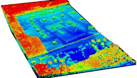
Takes the 17th flight strip as an example, the single flight strip is about 8 kilometres in length and 450 metres wide covering the area of 3.6 km2. The three channels point clouds have the following properties. In C1 channel, there are 23,609,034 points with an average point density of 6.5pts/m2 and an average point distance of 0.35 metre. In C2 channel, there are 23,321,813 points with an average point density of 6.5pts/m2 and an average point distance of 0.35 metre. In C3 channel, there are 16,920,213 points with an average point density of 4.7pts/m2 and an average point distance of 0.55 metre.
Figure 2. A subset of the 17th flight strip in town of Ballantrae
Figure 2 shows a subset of the 17th flight strip as test dataset. The subset is about 710m x 450m in a large town of Ballantrae, ON, Canada. The subset area mainly includes nine types of object features such as water bodies, bare soil, lawn, road, low vegetation, medium vegetation, high vegetation, building and power line for 3D land cover classification.
4. OBIA CLASSIFICATION METHOD
In this paper, an Object Based Image Analysis (Blaschke T., 2010) approach is presented using multispectral Lidar point clouds for 3D land cover classification. The main idea is that multispectral
Lidar point clouds are segmented and classified on the basis of return signal intensity images from the three channels raw data. The intensity depends on the reflectance of the ground material and laser pulse wavelength. Numbers of all returns point clouds, and elevation information from maximum first returns and minimum last returns are main factors for classification. Meanwhile, different objects reflective characteristic in three channels are taken into account for classification. Water is best penetrated in green spectrum, and a slightly reflective in NIR and IR spectrum. Power line is strongly reflective in NIR and IR spectrum and slightly reflective in green spectrum. Vegetation is strongly reflective in NIR spectrum, and slightly reflective in visible green spectrum. Soil is best reflective in intermediate infrared. Vegetation can be easily distinguished from soil and water.
The OBIA approach for 3D land cover classification consists of three steps. The first step is multi-resolution segmentation based on intensity layers of multispectral point clouds. Image objects are created via multi-resolution segmentation integrating large scale parameter for vegetation segmentation. To road and building, image objects are segmented with small scale parameter from the non-vegetation objects. To bare soil and lawn, image objects are segmented with large scale parameter from unclassified objects. Because different features have different boundary characteristic, we select different scale parameters to separate imagery objects. The second step is image objects classification of multispectral point clouds. The objects classes typically discerned 3D land cover classification in study area have nine different classes from bottom to up: water bodies, bare soil, lawn, road, building, low vegetation, medium vegetation, high vegetation and power line. The objects classes are attributed with a high-dimensional feature space, such as object vegetation index feature (pseudo NDVI, ratio of green), point cloud-related attribute (intensity, elevation, number of points, return number, class), and object statistics feature (brightness, area). Using these feature indexes, point cloud objects can be classified and linked to a hierarchical network, and a rule set of knowledge decision tree is created for classification. The last step is to assess the validity of classification results. Accuracy assessment is performed by comparing randomly distributed sampled points in reference imagery from Google map with the classification results.
4.1 Definition for Classification Indexes
Due to the limited availability of metadata, we define classification indexes as pseudo normalized difference vegetation index (pNDVI), ratio of green (RATIO_GREEN), ratio of returns counts (RATIO_COUNT), difference of elevation between maximum elevation of first returns and minimum elevation of last returns (DIFF_ELEVA) for classification of multispectral point clouds. The customized features are used to calculate different classification indexes as equation (1), (2), (3) and (4) respectively.
� � =� −�� +� (1)
�� � _ � =� +� +�� (2)
�� � _ = � � (3)
� _ � = ���� �� � − ���� �� � (4)
where C1 = intermediate infrared channel (1550nm) C2 = near infrared channel (1064 nm) C3 = green channel (532nm)
DIFF_ELEVA = difference of elevation
RATIO_COUNT = ratio of point counts from returns RATIO_GREEN = ratio of green band
pNDVI = pseudo normalized difference vegetation index
The Normalized Difference Vegetation Index (NDVI) is an effective threshold to a differentiation of vegetation and non-vegetation, which is derived from the red and near infrared bands (Rouse, et al., 1973; Nathalie, Pettorelli., 2013). Due to lack of red band of multispectral point clouds, Wichmann V. (2015) presented a pseudo NDVI. The combination red=C2, green=C3, blue=C1 is used to simulate a colour infrared similar visual appearance. The intensity values are used to create false colour composites for each point. The pNDVI is calculated with channels C2 (NIR) and C3 (Green). Ratio of Green (RATIO_GREEN) is a percentage of the green channel to the whole three channels. Ratio of counts returns (RATIO_COUNT) is a ratio between counts points from all returns and points counts from last returns. The value of ratio of returns counts is greater than or equal to 1. Difference of elevation (DIFF_ELEVA) is difference values between maximum elevation values from first returns of point clouds and minimum elevation values from last returns of point clouds, which expresses height information of the identical object.
4.2 Intensity Imagery Segmentation
We use eCongition Developer software (eCognition, 2014) to execute the multispectral point clouds segmentation and classification based on an OBIA approach. Image segmentation is the subdivision of three channels intensity layers into separated object regions, which meet certain criteria of homogeneity and heterogeneity. Segmentation criterion is to use different scale parameters with a combination of the spectral and shape properties in smoothness and compactness. The multi-resolution segmentation approach allows for nested segmentation at different scale parameters. A hierarchical network of image objects can be constructed by repeating the segmentation with different scale parameters. Each image object is encoded with its hierarchical position, its membership and its neighbours (Benz et al., 2004; eCognition, 2014). Intensity image objects are grouped until a threshold representing the upper object variance is reached. The scale parameter is weighted with separation of shape and compactness parameters to minimize the fractal borders of the objects.
We use three times multi-resolution segmentations and once spectral difference segmentation in the study. In the initial segmentation, we use multi-resolution segmentation to create image objects primitives from intensity layer of point clouds. We select a group of parameters, which scale parameter is equal to 5, shape parameter 0.5 and compactness parameter 0.5 for identifying vegetation from other objects. The weighting of NIR (C2) image layer has been increased to 2 because vegetation has strongly reflective in NIR spectrum. The weightings of IR (C1) and Green (C3) image layers are increased to 1. Larger scale segmentation makes homogeneity objects keep good connectivity to grow neighbouring pixels. In the second multi-resolution segmentation, we select smaller scale parameter is equal to 1, shape parameter 0.5 and compactness parameter 0.5 for determining detail boundary of road and building. The weighting of IR (C1), NIR (C2) and Green (C3) image layers has been increased to 1. Smaller scale segmentation makes homogeneity objects keep good independence in order to reduce
the influence of heterogeneity objects. In the third multi-resolution segmentation, we select scale parameter is equal to 5, shape parameter 0.5 and compactness parameter 0.5 for distinguishing lawn and bare ground. The weighting of NIR (C2) image layer is setup to 2, and the weightings of IR (C1) and Green (C3) image layers are setup to 1. And then, we use the spectral difference segmentation to merge neighbouring image objects with a maximum spectral difference mean below the threshold. The neighbouring image objects are merged to produce the final objects if the difference between their layer mean intensity is less than 10. The larger scale segmentation and spectral combination makes lawn and bare ground objects keep good neighbouring relationship. Figure 3 illustrate the results of twice multi-resolution segmentation using different scale parameter 5 and 1. There are many larger separated areas in vegetation and many smaller separated areas in road, building and other objects areas.
Figure 3. Results of twice multi-resolution segmentation using different scale parameter 5 and 1
4.3 Classification
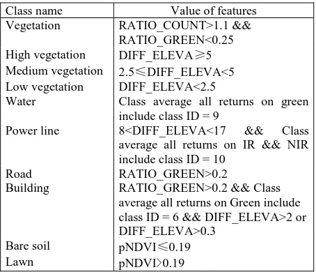
To identify the intensity images objects as certain 3D land cover classes, we define nine categories from bottom to up as water bodies, bare soil, lawn, road, low vegetation, building, power line, medium vegetation and high vegetation according to terrain analysis of study area. A knowledge base of classification rules is constructed to classify each object into certain class, and a knowledge process tree is formed. To classify the relevant objects, the threshold of objects is determined by quantitative analysis using object related features information. Objects characteristics such as pNDVI, RATIO_GREEN, RATIO_COUNT, DIFF_ELEVA, point cloud-related attribute, spatial relation and statistical measures are utilized to create the knowledge rules for classification. Table 1 lists briefly the class hierarchy, object class, rule sets of knowledge based process tree and value of feature (thresholds) based on OBIA approach. In table 1, class average all returns on green include standard class (ID=6) means building class from point clouds. Class average all returns on Green include standard class (ID=9) means water class from point clouds. Class average all returns on IR && NIR include standard class (ID=10) means power line class from point clouds in IR and NIR channels.
4.3.1 Vegetation classes: These object primitives can be assigned to vegetation class after initial segmentation. By quantitative analysis to test the threshold of classification indexes, vegetation objects class is first identified if RATIO_COUNT is greater than 1.1 and RATIO_GREEN is less than 0.25. Height information from a maximum elevation from first returns and a minimum elevation from last returns data is used to identify The International Archives of the Photogrammetry, Remote Sensing and Spatial Information Sciences, Volume XLI-B1, 2016
different height vegetation. Vegetation objects are classified into three classes such as high vegetation, medium vegetation and low vegetation. High vegetation can be distinguished from vegetation if DIFF_ELEVA is greater than 5 meter using the difference of elevation between maximum elevation of first returns and elevation minimum of last returns. Medium vegetation can be assigned from vegetation if DIFF_ELEVA is greater than 2.5 meter and less than 5 meter. Low vegetation can be distinguished from vegetation if DIFF_ELEVA is less than 2.5 meter.
Class name Value of features
Vegetation RATIO_COUNT>1.1 && RATIO_GREEN<0.25 High vegetation DIFF_ELEVA 5 Medium vegetation 2.5 DIFF_ELEVA<5 Low vegetation DIFF_ELEVA<2.5
Water Class average all returns on green include class ID = 9
Power line 8<DIFF_ELEVA<17 && Class average all returns on IR && NIR include class ID = 10
Road RATIO_GREEN>0.2
Building RATIO_GREEN>0.2 && Class average all returns on Green include class ID = 6 && DIFF_ELEVA>2 or DIFF_ELEVA>0.3
Bare soil pNDVI 0.19
Lawn pNDVI>0.19
Table 1. Class hierarchy and rule sets based on OBIA approach
4.3.2 Road and Building classes: After vegetation is classified, the second segmentation is performed from unclassified non-vegetation objects by small scale parameter. These objects of road and building classes can be divided from unclassified objects. The road class is assigned if RATIO_GREEN is greater than 0.2. All buildings have been misclassified to road class because the road and building has similar spectral characteristic. To identify the building from road, we firstly use DIFF_ELEVA index to distinguished building if DIFF_ELEVA is greater than 2 meter. We find only the edge points of building can be separated. Roof points of building can’t be separated from the road and the value of DIFF_ELEVA in roof points is greater than 0.3 meter. Without other ancillary data, we use the manual classification to determine buildings category. The buildings of Lidar datasets are classified into the standard class (ID=6). The 6th class belongs to building category of raw point clouds. We combine the value of DIFF_ELEVA index with point-clouds related class to identify the building class using class ID=6 of class average all returns on green. Finally, the building class is assigned and can be identified from the road.
4.3.3 Water class: The intensity value of water body only exists on C3 channel including water bottom and water surface. There are dark holes in NIR and IR channels that mean the laser of NIR and IR bands are completely absorbed by water, and no point clouds data. Without other ancillary data, we use the manual classification to determine water category. The water bodies of Lidar datasets are assigned by point-clouds related class of raw point clouds using class ID=9 average all returns on green band.
4.3.4 Power line class: The intensity value of power line exists on C1 and C2 channel. There are no point clouds data in C3 channel. The height information is between 8 and 17 meters. Without other ancillary data, we use the manual classification to determine power line category. The power line of Lidar datasets are classified in the standard class (ID=10) of raw point clouds. The power line class is assigned by point-clouds related class ID=10 of class average all returns on NIR and IR bands.
4.3.5 Bare soli and lawn classes: To unclassified intensity objects layers, the third multi-resolution segmentation and spectral difference segmentation are performed with large scale parameter and spectral difference threshold. Neighbouring spectrally similar intensity objects are merged. The object of bare soil class can be identified from unclassified objects if pNDVI is less than or equal to 0.19. And then, lawn class is assigned from unclassified objects if pNDVI is greater than 0.19.
4.3.6 Other processing methods: Many of other approaches based on OBIA are used to clean up the classified objects for refining the classification results such as merge region, find enclosed by class, pixels area and so on. To the same objects class, the merge region algorithm on classified objects is used to merge these regions. We use find enclosed by class to assign both unclassified objects and no point clouds area or misclassification objects to the corresponding classes if area pixel is less than 5 pixels.
4.4 Accuracy Assessment
Accuracy assessment can produce statistical outputs to evaluate the quality of classification results. More than two hundred randomly distributed sampled points are created on downloaded imagery from Google Earth (Google Earth, 2016). The google imagery has completely registered with the intensity image layers. Each of these sampled points is labelled to its proper class by visual human interpretation of google earth imagery, forming the reference dataset. These reference points are compared with classification results at the same locations. We use these known reference points to assess the validity of the classification results, to calculate a confusion matrix, to derive the user’s accuracy and producer’s accuracy for each class, to calculate errors of commission and omission for each class, and to compute an overall accuracy and kappa statistics for the classification results. User’s accuracy and producer's accuracy, commission error and omission error, over accuracy and kappa coefficient computed and the equations comes from these references (Congalton, R.G., 1991; Jensen, J.R., 1996).
5. RESULTS AND ANALYSIS
5.1 Results of Classification and Accuracy Assessment
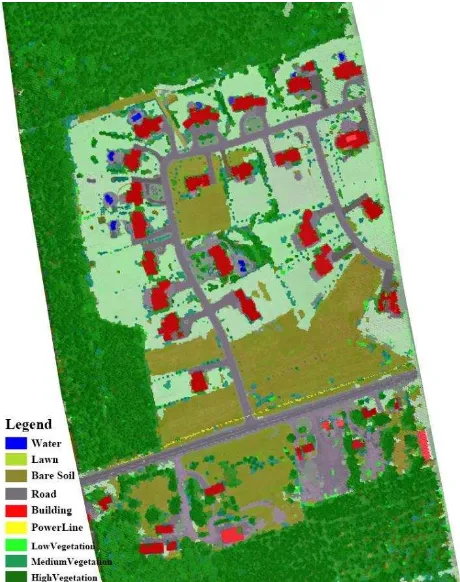
The study area is classified into main nine classes for 3D land cover classification. The objects classes are water bodies (blue), bare soil (olive), lawn (beryl green), road (grey), low vegetation (light green), medium vegetation (malachite green), high vegetation (dark green), building (red) and power line (solar yellow). Figure 4 shows the classification results for nine classes based on OBIA approach using multispectral point clouds. The accuracy assessment of the classification results for nine classes is performed using a total number of 203 randomly distributed sampling point data. The overall accuracy (OA) of OBIA classification reaches 91.63% in the study area and the Kappa coefficient is recorded as 0.895. The confusion matrix for nine classes is listed in Table 2 and the error statistics and overall The International Archives of the Photogrammetry, Remote Sensing and Spatial Information Sciences, Volume XLI-B1, 2016
accuracy for nine classes is listed in Table 3 in accuracy assessment.
Figure 4. Classification results of nine classes in study area
Object Classes
Reference Points from Google Imagery
HV MV LV BU RD BS LA WA PL RT HV 68 3 0 0 0 0 0 0 0 71 MV 1 11 0 0 0 1 1 0 0 14 LV 0 0 8 0 0 0 0 0 0 8 BU 0 0 0 12 0 0 0 0 0 12 RD 1 0 0 1 26 0 2 0 0 30 BS 0 1 0 0 1 26 0 0 0 28 LA 0 1 1 0 1 2 33 0 0 38 WA 0 0 0 0 0 0 0 1 0 1
PL 0 0 0 0 0 0 0 0 1 1 CT 70 16 9 13 28 29 36 1 1 203
Note
HV=high vegetation, MV=medium vegetation, LV=low vegetation, BU=building, RD=road, BS=bare soil, LA=lawn, WA=water, PL=power line, RT= row total, CT=column total
Table 2. The confusion matrix for nine classes
Object Classes
User’s Accuracy (%)
Commission Error (%)
Producer's Accuracy (%)
Omission Error (%) HV 95.77 4.23 97.14 2.86 MV 78.57 21.43 68.75 31.25 LV 100 0 88.89 11.11 BU 100 0 92.31 7.69 RD 86.67 13.33 92.86 7.14 BS 92.86 7.14 89.66 10.34 LA 86.84 13.16 91.67 8.33 WA 100 0 100 0
PL 100 0 100 0 Accuracy
Assessment
Overall
Accuracy 91.63%
Kappa
Coefficient 0.895
Table 3. The error statistics and overall accuracy
5.2 Results Analysis
Various objects are generated using the different weighting of intensity imagery layers from multispectral point clouds data
through three time multi-resolution segmentation and once spectral difference segmentation. Nine object classes are assigned for classification. The threshold of classification is determined by quantitative analysis and the customized classification indexes for identifying objects feature classes. Most of object classes can be well distinguished by using classification indexes or spectral feature. Difference in height from a maximum elevation from first returns and a minimum elevation from last returns plays a vital role in identifying the vegetation classes. Ratio of green is a key factor to distinguish the vegetation, road and building. A pseudo NDVI is applied to separate bare soil and lawn. Height information and standard classes of point clouds are used to divide the building and road. To water and power line, we use point clouds segmentation to distinguish these objects. It makes the objects of water bodies in C3 channel and power line on C1 and C2 channels identify easily and accurately. Most of objects have been classified correctly and completely for 3D land cover classification. However, there exists a few of misclassification objects. A small path is misclassified to bare soil instead of road because it has soil property. Many of misclassifications happen at spectral similar area such as high vegetation and medium vegetation, between bare soil and lawn. Some misclassifications happen at the obscure boundary of different objects types due to nearly identical spectral features and lack of effective spectral and spatial feature to distinguish such as between road and bare soil, between road and lawn.
6. CONCLUSION
The object based image analysis (OBIA) approach is an effective way to classify the multispectral Lidar point clouds data for 3D land cover classification. The definition of classification indexes in paper is very attractive for the separation of different height vegetation and spectral similar objects point clouds. Repeating the segmentation with different scale parameters make the boundaries of 3D land cover types distinguish from other objects features easily. For evaluating the classification results, confusion matrix and error statistics for nine classes are calculated, and overall accuracy is as high as 91.63% and Kappa Coefficient reaches 0.895. Multispectral Lidar system is a new promising research domain, especially in applications of 3D land cover classification, seamless shallow water bathymetry, forest inventory and vegetative classification, disaster response and topographic mapping. Further research is needed to combine multispectral Lidar point clouds with other ancillary data such as digital surface model (DSM) and imagery in order to improve the associated precision.
ACKNOWLEDGEMENTS
The authors would like to thank Teledyne Optech Inc. for provision of the test dataset from the multispectral Lidar system Optech Titan and in particular Mr. Xing Fang for the technical support. We are very grateful to China Scholar Council for the support to the study. Thanks to the participants in State Key Laboratory of Geo-Information Engineering for many helpful comments. Thanks Professor Jonathan LI in University of Waterloo for suggestion.
REFERENCES
Ahmed, Shaker., Paul, LaRocque. and Brent, Smith., 2015. The Optech Titan: A Multi-Spectral Lidar for Multiple Applications. JALBTCX Workshop. http://shoals.sam.usace.army.mil/ The International Archives of the Photogrammetry, Remote Sensing and Spatial Information Sciences, Volume XLI-B1, 2016
Workshop_ Files/2015/Day_01_pdf/1130_LaRocque.pdf, pp. 1-56 (Accessed 12 March 2016).
Bakuła, Krzysztof., 2015. Multispectral Airborne Laser Scanning - a New Trend in the Development of Lidar Technology. Archiwum Fotogrametrii, Kartografii i Teledetekcji, 27, pp. 25-44.
Benz, U.C., Hofmann, P., Willhauck, G. and Lingenfelder, I., 2004. Multi-Resolution, Object-Oriented Fuzzy Analysis of Remote Sensing Data for GIS-Ready Information. ISPRS Journal of Photogrammetry and Remote Sensing. Elsevier, Amsterdam, 58, pp. 239–258.
Blaschke, T., 2010. Object Based Image Analysis for Remote Sensing. ISPRS Journal of Photogrammetry and Remote Sensing, 65(2), pp. 1-16.
Congalton, R.G., 1991. A Review of Assessing the Accuracy of Classifications of Remotely Sensed Data. Remote Sens. Environ. 37, pp.35-46.
Doneus M., Miholjek I., Mandlburger G., Doneus N., Verhoeven G., Briese C. and Pregesbauer, M., 2015. Airborne Laser Bathymetry for Documentation of Submerged Archaeological Sites in Shallow Water. International Archives of Photogrammetry, Remote Sensing and Spatial Information Science, 1, pp. 99-107.
eCognition, 2014. Trimble eCognition Developer User Guide (Version 9.0).pdf, Website: www.eCognition.com (Accessed 16 February 2015).
Google Earth, 2015. Google Maps and Google Earth for Desktop (Version 7.1.5.1557) Software. 2015 Google Inc., https://www.google.com/earth/explore/products/desktop.html (Accessed 1 April 2016).
Irish, J. L., and Lillycrop, W. J., 1999. Scanning Laser Mapping of the Coastal Zone: the SHOALS System. ISPRS Journal of Photogrammetry and Remote Sensing, 54(2), pp. 123-129.
Jensen, J. R. 1996. Introductory Digital Image Processing: A Remote Sensing Perspective (Second edition). Prentice Hall, Upper Saddle River, New Jersey07458, USA, pp. 247-252.
Leica HawkEye III, 2015. Airborne Hydrography AB HawkEye III. https://www.airbornehydro.com/hawkeye-iii/Leica AHAB HawkEye DS.pdf, pp. 1-2 (Accessed 20 March 2016).
Michael R. Sitar, 2015. Multispectral Lidar and Application Opportunities. GeoSpatial World Forum 2015, Portugal, pp. 1-35. http://geospatialworldforum.org/speaker/SpeakersImages/ Michael20Sitar.pdf (Accessed 8 March 2016).
Nathalie, Pettorelli., 2013. The Normalized Difference Vegetation Index (First Edition), Oxford University Press, Oxford, United Kingdom, pp. 18-29.
Rouse, J.W., Haas, R.H., Schell, J.A. and Deering, D.W., 1973. Monitoring Vegetation Systems in the Great Plains with ERTS. 3rd ERTS Symposium, NASA SP -351, Washington DC, 10-14 December, pp. 309-317.
Titan Brochure and Specifications, 2015. Optech Titan Multispectral Lidar System - High Precision Environmental Mapping. http://www.teledyneoptech.com/wp-content/uploads /Titan-Specsheet-150515-WEB.pdf, pp. 1-8 (Accessed 12 January 2016).
Valerie, Ussyshkin., Livia, Theriault., 2011. Airborne Lidar: Advances in Discrete Return Technology for 3D Vegetation Mapping. Remote Sensing, 3(1), pp. 416-434, http://www.mdpi. com/journal/remotesensing (Accessed 14 January 2016).
Wang, C. K., Tseng, Y. H. and Chu, H. J., 2014. Airborne Dual-Wavelength LiDAR Data for Classifying Land Cover. Remote Sensing, 6(1), pp. 700-715.
Wichmann, V., Bremer, M., Lindenberger, J., Rutzinger M., Georges, C. and Petrini-Monteferri, F., 2015. Evaluating the Potential of Mutispectral Airborne Lidar for Topographic Mapping and Land Cover Classification. ISPRS Annals of the Photogrammetry, Remote Sensing and Spatial Information Sciences, Volume II-3/W5, ISPRS Geospatial Week 2015, La Grande Motte, France., pp. 113-119.
Wikipedia, 2016. Whitchurch-Stouffville, Town Ontario, Canada from Wikipedia, the Free Encyclopedia and Statistics Canada, 2012-02-08,https://en.wikipedia.org/wiki/Whitchurch-Stouffville (Accessed 22 March 2016).