AIRBORNE CROWD DENSITY ESTIMATION
Oliver Meynberg∗
, Georg Kuschk
Remote Sensing Technology Institute, German Aerospace Center (DLR), 82234 Wessling, Germany (oliver.meynberg, georg.kuschk)@dlr.de
Commission III/VII
KEY WORDS:Crowd detection, Aerial imagery, Gabor filters, Texture features
ABSTRACT:
This paper proposes a new method for estimating human crowd densities from aerial imagery. Applications benefiting from an accurate crowd monitoring system are mainly found in the security sector. Normally crowd density estimation is done through in-situ camera systems mounted on high locations although this is not appropriate in case of very large crowds with thousands of people. Using airborne camera systems in these scenarios is a new research topic. Our method uses a preliminary filtering of the whole image space by suitable and fast interest point detection resulting in a number of image regions, possibly containing human crowds. Validation of these candidates is done by transforming the corresponding image patches into a low-dimensional and discriminative feature space and classifying the results using a support vector machine (SVM). The feature space is spanned by texture features computed by applying a Gabor filter bank with varying scale and orientation to the image patches. For evaluation, we use 5 different image datasets acquired by the 3K+ aerial camera system of the German Aerospace Center during real mass events like concerts or football games. To evaluate the robustness and generality of our method, these datasets are taken from different flight heights between 800m and 1500m above ground (keeping a fixed focal length) and varying daylight and shadow conditions. The results of our crowd density estimation are evaluated against a reference data set obtained by manually labeling tens of thousands individual persons in the corresponding datasets and show that our method is able to estimate human crowd densities in challenging realistic scenarios.
1 INTRODUCTION
Monitoring large crowds is an important topic in the field of se-curity surveillance as it can provide crucial information for de-cisions by the local security forces, as for example detecting a hazardous situation which may result in a panic. For mass events with thousands of people, the only feasible method for crowd monitoring is by airborne camera systems, due to sheer scale and the limited field of view from in-situ cameras. Manual crowd estimation by human observers is possible when enough trained experts are at hand, but in general this is not the case and often also a question of costs and time. Therefore it is highly desirable to employ airborne camera systems which are able to monitor hu-man crowds at such large events.
For ground based scenarios, (Lin et al., 2001) train a classifica-tion system on head-like contours to detect and count people in indoor scenarios. For this system to work, the camera needs to be roughly on the same height like the observed people, resulting in the same limited field of view as for a human observer in the same situation, and is therefore only applicable for small indoor scenarios. The work (Ghidoni et al., 2012) uses co-occurence matrices of the input images to measure change in image texture. As this method is not invariant in scale, rotation or even intensity, this method only works for stationary cameras as for example in stadiums. A very good work done by (Arandjelovic, 2008) uses a sliding window approach in scale space to create a bag-of-words descriptor for each image patch using clustered SIFT features and classifying them using a SVM. However, their result is just a bi-nary crowd mask and the evaluation is done by comparison w.r.t. a hand-segmented ground truth, and ergo has quite a strong sub-jective bias towards the labeling persons definition of a crowd. In a different terrestrial setup, (Aswin C et al., 2009) are using a multi camera setup and background subtraction to detect single persons (and classifying their activities using pre-learned linear dynamical systems).
In the field of aerial crowd detection and crowd density
estima-tion, (Hinz, 2009) uses sequences of temporally consecutive and overlapping images to estimate the background by applying a gray-level bounded region-growing approach. Then, a blob de-tector (in the paper called Laws texture filter) is used on the fore-ground pixels to filter out non-crowd-like objects. To estimate the crowd density, a Gaussian smoothing kernel with a fixed standard deviation / bandwidth is applied. This is an often used approach for density estimation which we slightly adjust to our needs. Un-fortunately, a quantitative evaluation is missing. In the work of (Sirmacek and Reinartz, 2011), the FAST feature detector is ap-plied to detect blob-like and corner-like image structures. To filter out non-crowd / non-people responses in highly cluttered back-ground, in a second step image segmentation is used to remove segmented areas which are too small (crowds are assumed to be placed atop of a uniform looking surface) and which contain less than a certain amount of local features. This approach seems to work well when the parameters are tuned to a given dataset, but it is clearly non scale or color/contrast invariant, as the chosen parameters for the image segmentation algorithm and the thresh-olds for the number of local features and minimum area size need to be tuned for every dataset anew. However, the herein proposed method of determining the bandwidth for the kernel density es-timation via the mean of the minimum nearest distances of the detected people gives promising results for estimating the crowd density.
2 METHOD
consist of an agglomeration of such structures.
In a second step we extract image patches around these interest points and extract scale- and rotational invariant texture feature descriptors by Gabor filtering these image patches. The result-ing feature descriptors are classified by a support vector machine (Drucker et al., 1997) and the positively classified crowd areas are then used to estimate a crowd density for the whole image, based on kernel density estimation with an automatically com-puted kernel bandwidth.
For filtering out non-crowd image patches in the second step it is of course also possible to use additionally provided road maps, building footprints or digital elevation models, but as this data usually is not available to the local operators and would restrain the usage of our method, we do not consider these options. Fur-thermore we decided against a single person detection, as the re-sults would be highly unreliable using typical nowadays aerial imagery taken from a law-regulated flight altitude of 1000-1500m, where a person seen from directly atop covers roughly 5-10 im-age pixels (see Figure1for examples).
The single components of our complete workflow are as follows
1. Detect FAST featuresFk∈Ω
2. Extract image patchesIkaroundFk
3. Create texture feature descriptorsvkby Gabor filteringIk
4. Classifyvkusing a trained SVM
5. Estimate crowd density based on positive detections
and will be described in detail in the following sections.
2.1 Interest Point Detector
To restrict the search range for image patch based classification from all possible pixel positions (e.g. 21MPix) to a small number of probable candidates (50,000), we first apply an interest point detector as a very rough but fast initial filtering of all image posi-tions into regions possibly containing crowd areas or non-crowd areas. The design of the interest point detector does not need to be overly complicated, as long as it detects local image in-tensity changes (see the characterization of crowd areas in the following Section2.2). Further, we do not want to detect in-tensity changes along regular edges, but to detect blob-like and corner-like small elements. Typical operators for this task are the Harris corner detector (Harris and Stephens, 1988) or the Lapla-cian of Gaussian. However, the FAST corner detector (Rosten and Drummond, 2006) was specifically designed to detect these points of interest in a minimum of computational time, which is why we use these FAST features for initial filtering of possible crowd areas.
2.2 Feature Extraction
Seen from an aerial observer’s side, a human crowd is charac-terized by an image region containing a number of very small subregions which are differing in brightness or color from their surrounding. These subregions or blobs should be further ran-domly distributed (ranging from dense to sparse), exhibiting no recognizable pattern (see Figure1for typical examples). And as we are interested in crowd detection only, all other image regions are deemed to not contain crowds.
We thus need to transform this intuitive characterization of prop-erties of an image patchI ∈ RM×N into a formal operatorF, with which we can automatically compute a distinctive and reli-able feature spaceRd
F :RM×N →Rd (1)
The resultingd-dimensional feature space should have low intra-class variability (one crowd area should result in a similar feature vector as a completely different crowd area) and a high interclass variability (feature vectors of crowd areas should be distinct from feature vectors from non-crowd areas).
(a) High crowd density plus shad-ows
(b) Low image resolution and low contrast
Figure 1: Examples of 64×64 image patches containing human crowds in a challenging aerial imagery. A reliable estimation of single persons is not possible due to the low image resolution.
Gabor filters are a highly suitable choice for the transformation
F, with their frequency and orientation representations being sim-ilar to the human visual system. Introduced to computer vision by (Daugman et al., 1985) and (Daugman, 1988) they have been found to be particularly appropriate for texture representation and discrimination. Usage ranges from retrieval of image data, e.g. (Manjunath and Ma, 1996) and (Han and Ma, 2007), to optical character recognition (Wang et al., 2005) and fingerprint feature extraction (Lee and Wang, 1999), just to name a few.
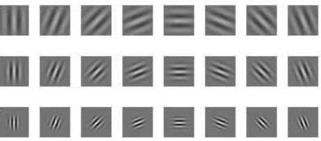
A 2D Gabor filter is a Gaussian kernel function modulated by a sinusoidal wave in a specified direction (Figure2), with the re-sponse of a 2D image convolution being highest for image gra-dients along the filters orientation. Simply speaking, Gabor fil-ters are detecting image gradients of a specific orientation. The convolution of image patches with a number of different scales and orientations allows for extraction and encoding of local tex-ture information into a low dimensional featex-ture vector, usable for generic classification.
The motivation behind our choice of Gabor filters is that a crowd area, having the aforementioned characteristics of randomly dis-tributed blobs, should give a high response in every direction, whereas regular man made structures only have high responses orthogonal to their main orientations and natural structures should give a similar response in every direction, but due to lack of con-trast of a lower magnitude than for crowds.
As their definitions are manifold, and in order for this paper to be self-contained, we describe our choice of Gabor filters used throughout the rest of the paper in the following:
The mother wavelet of the two-dimensional complex Gabor
tions is defined as
The real and imaginary parts of this wavelet are computed as
gre(x, y) =G(x, y)·cos(2πW x)
gim(x, y) =G(x, y)·sin(2πW x) (4)
A filter bank of gabor functionsgs,k(x, y)is now generated by rotating and scaling the mother waveletg(x, y)as follows
gs,k(x, y) =a ber of orientations, and the scaling factora−sassuring that the energy of the filter is independent of the scales = 0, .., S−1
(Sbeing the number of scales). Following the argumentation of (Manjunath and Ma, 1996) to reduce the redundancy of the re-sulting nonorthogonal Gabor wavelets, we seta= (Uh/Ul)1/S, resulting inW = Uh/aS
−s
. The upper and lower center fre-quency of interest are set toUh= 0.4, Ul= 0.1andσx, σyare set accordingly.
Given an image patchI ∈RM×N
, its Gabor wavelet transform is now defined as
The corresponding texture attributes for one such wavelet trans-form, given a scalesand orientationk, are computed as the mean and standard deviation of the absolute valued filter response
µ(s,k)=
and the full feature vectorf constructed by applying a whole filter bank of Gabor wavelets (e.g. S = 3andK = 8) to the image patchIand concatenating the resulting attributes to a 48-dimensional vector
f(i) =
µ(0,0), σ(0,0), µ(0,1), . . . µ(2,7), σ(2,7)
(8)
encoding, laxly speaking, the amount of edges in a number of different orientations. Note that due to taking the absolute value of the filter response, it does not matter whether a person appears dark on bright background or vice versa.
As a naive 2D convolution of image patchesI∈RN×Nwith Ga-bor filtersg∈RM×M
would result in an intractable complexity ofO(N2M2), we transform both the image patch and the fil-ter from spatial domain to frequency domain by the fast Fourier transform, multiply the elements pointwise and transform the
re-sult back to obtain our feature attributes, rere-sulting in a complexity ofO(N2logN2+M2logM2). For typically sized image patches I ∈R64×64
and Gabor filtersg∈R32×32
the speedup factor is around factor 70. We further sped up the algorithm by precom-puting the FFT’s of the different Gabor filters only once and by making use of multi core parallelization. The border pixels of an image patch need to be treated with care, both in the spatial and frequency domain. Therefore, before computing the Fourier transform, we apply a windowing function to the input image, to reduce the ringing effects. Note that in the spatial domain we would have similar problems.
2.3 Classification
As we cannot assume our feature vectors to be linear separable with respect to their classes, statistical distance measures like the Mahalanobis distance would perform quite bad. In constrast, kNN classifiers (k nearest neighbors) are fully capable to handle multimodal distributions in the feature space, but are quite sensi-tive to overlapping / mixed distribution class areas. Support vec-tor (regression) machines (SVM) (Drucker et al., 1997) instead are combining both of the aforementioned advantages, as they are specifically designed for non-linear classification and, based on statistical regression, are robust to areas of overlapping class distributions. The only care has to be taken for highly imbalanced training data, where the number of positive samples of one class is much larger than the other classes. Simple over-sampling (syn-thetically generating positive samples) is taking care of this issue though.
2.4 Crowd Density Estimation
To estimate a crowd density based upon our classification results, we consider the crowd density as a probability density function (pdf) over the image domain. Since the classification results pro-vide only a finite and very sparse set ofN sampled data points of this pdf, we need to apply additionally data smoothing in-between, inferring about the real underlying pdf. A standard method to this end is the kernel density estimation, defined as
fh(x) = 1
with the kernel functionKtypically being a Gaussian distribu-tion. The only problem here is the choice of the smoothing pa-rameter (also called bandwidth)h. As the crowd detection algo-rithm is required to work on images of different scale, the size and distances between two identical image features can vary in image space, when the images are taken from different distances in world space or with a different image resolution. Therefore, an automatic data-driven bandwidth selection is needed, adapting for every image or scale respectively.
3 EVALUATION
Instead of hand-segmenting human crowds and comparing a com-puted binary crowd mask, we evaluate the accuracy of the esti-mated crowd density in a continuous way without applying any thresholds. We choose this approach because in reality there is also no artificial threshold where you distinguish between certain crowd density levels. Our proposed method uses original, not-orthorectified JPEG images and does not rely on additional in-formation like road maps or building plans as our method should work ad-hoc without additional preprocessing steps.
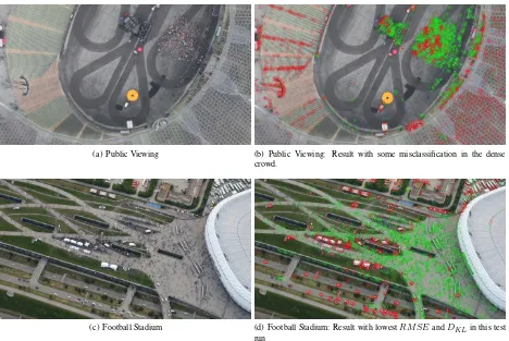
(a) Public Viewing (b) Public Viewing: Result with some misclassification in the dense crowd.
(c) Football Stadium (d) Football Stadium: Result with lowestRM SEandDKLin this test run
Figure 3: Test images with classification results of the detected interest points. green ˆ= classified as crowd, red ˆ= classified as non-crowd
Each camera has a full frame CMOS sensor with a resolution of 21 MPix. The used lenses are a Zeiss Makro Planar 2/50mm and a Zeiss Distagon T 2/35mm.
3.1 Test Data
Evaluation of the proposed algorithms is done on five different aerial image datasets (see Table1). The City Centre dataset con-sists of three images showing the crowded shopping streets around Munich’s New Town Hall on a sunny day. While the individual persons and their shadows are clearly visible, other regions in the image consist of small dense crowds where single persons occlude each other. Due to the lower flight altitude the Public Viewing data set has a slightly higher resolution. In some im-ages of this scene one large group sits on the ground of an arena in front of a screen and smaller but also dense groups stand in other areas (Figure3a). The lighting conditions are mixed with images containing shadows and no shadows respectively. The Southside data set shows images of a rock festival from two dif-ferent flight altitudes (1000m/1500m) and difdif-ferent angles. The scene has both dense crowds and individuals. The main challenge in this dataset is the huge campground with a lot of small tents. The interest point detector apparently detects all the corners of the tents which does not really lead to a reduction of the search space. Moreover individuals standing between tents can hardly be detected. The RockamRing dataset shows another rock festi-val with dense and sparse crowds (Figure6a, details in Section
3.2). It was acquired with an older camera system which is why the GSD is worse than in the other datasets. Finally, the images of the Football Stadium dataset show the crowded area in front of a stadium from a side-view perspective which results in varying GSDs. The reference data is acquired by manually marking each single person in the test images. The ”Images” column in Table
1indicates the number of manually marked images per data set, the ”Point of view” column indicates if the data set contains only nadir images or also images from a sideview perspective.
Dataset GSD [cm] Images Point of View
City Centre 13 3 nadir
Public Viewing 10 10 nadir/side
Southside 13/18 5 nadir/side
Rock am Ring 20 4 nadir
Football Stadium 10 (varies) 10 side
Table 1: Overview of the five different data sets.
3.2 Accuracy evaluation
We evaluate the accuracy of the classified images by comparing them with the reference images. Single persons in these reference images were labeled by different human interpreters. Then we apply the same image smoothing kernel as defined in Section2.4
on these reference images resulting in a Gaussian-filtered image with highest intensities at regions with the highest number of la-beled persons. To actually compare the pdfs of the reference and of the classified image we normalize both pdfs and convolve the image with the same Gaussian kernel. Both resulting images are represented byP andQin the following. Without loss of gen-erality the kernel’s radius and standard deviation were selected beforehand, based on the choice of different human interpreters who decided which number of persons per area is sufficient to regard a specific area as crowded.
For similarity measurement we calculate the mean absolute error
M AE= 1
n PN
RM SE= n1 between the classifiedP and the respective reference imageQ.
DKL ∈ [0,∞)whereDKL = 0meansP = Q. Apparently, the smaller the errors are the more similar the images are and the better is the classification result.
The classifier training runs on one manually selected image of the dataset with a certain parameter combination which the classifier uses for all images in the dataset. Then, this procedure of training and classifying with the same parameters repeats for many com-binations. Concretely, we tried Gabor filters with different scales, orientations, filter radii, and image patch widths. The parameter ranges are listed in Table2. We tried all possible combinations in the given range with the constraint that the Gabor radius must not be bigger than half the width of an image patch.
Image Patch Width [pixel] 32, 48, 64, 80, 96 Gabor Filter Radius [pixel] 8, 16, 24, 32 Number of scales 2, 3, 4
Number of orientations 8,10,12,14,16,18,20,24
Table 2: Gabor filter parameters we used in the evaluation.
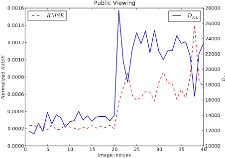
Figure4shows the resulting measures for the Publicviewing dataset. TheRM SEand theDKLare plotted for forty of the classified images. Images 1-20 have the lowestRM SEwhereas Images 21-40 have the highestRM SEof the whole test run which con-sists of several thousands of images due to the large number of possible parameter combinations. Table3lists the used parame-ters for these images. All three similarity measures often corre-late with each other and show that the lower these measures are the better is the classification result. Figure3shows the classifi-cation results with the lowest (=best) similarity measures of the whole Public Viewing dataset and the whole Football Stadium dataset, respectively.
Figure 4: RM SEandDKLfor the Publicviewing dataset. The steep slope between images 20 and 21 marks the border between images with lowest and highest errors.
TheDKLof the first three test images (No.1-3) for the Rockam-ring dataset is high although theM AE(not shown) andRM SE
are the lowest in this test run (Figure5and Table4).DKL mea-sures the difference between the two probability distributions of the classified and of the reference image. In the case of the test images No. 1-3 the chosen parameters perform badly and clas-sify all patches as ”non-crowd” and no patch as ”crowd” which results in a large difference of the pdfs and a largeDKL. Figure
No. gr scl ori pw No. gr scl ori pw
Table 3: Public Viewing dataset: The images with the lowest and highest similarity measures and the used Gabor filter
parameters.(No.= Image index which corresponds to the images in Figure4, gr=Gabor radius, scl=Number of scales,
ori=Number of orientations, pw=Patch width)
0 5 10 15 20 25 30 35 40
Figure 5:RM SEandDKLfor the RockamRing dataset. Note the largeDKLdifference between images No. 3 and No. 4, but a near constantRM SE.
No. gr scl ori pw No. gr scl ori pw
Table 4: Excerpt of Gabor parameters for highest and lowest sim-ilarity measure for the Rock am Ring dataset.
6b shows the bad result. Test Image No.4, however, has a low
DKLwhich corresponds to the visualization in Figure6c, which is much better. This is an unexpected result because how can a low RMSE be achieved for a misclassified image while for the same images theDKLis high - as expected for a wrong classifi-cation.
This case exemplarily shows the limits of this evaluation strategy, as a smoothing kernel might also remove relevant information. Another, potentially more intuitive approach, is to compare the number of manually counted people with the number of rightly classified, and detected corners per image tile.
4 CONCLUSION AND FUTURE WORK
(a) Input image (b) Misclassified image
(c) Reasonably good classified (green ˆ= crowd, red ˆ= non-crowd)
Figure 6: Figures b and c have a lowRM SEwhen compared to the reference image. However, while Figure b also has a low
RM SE it has a high DKL which helps us to understand the totally misclassified image. The result in Figure c is considerably better where bothRM SEandDKLare low.
Figure 7: Estimated crowd density (High image intensities corre-spond to high crowd densities.)
the resulting feature space after manual training. The quality of the results clearly depends on good training samples and similar images. The Gabor filter gives some good first results, however, a good global classifier has still to be found. In our future work Gabor filters will play a role in combination with other texture features. Another major aspect is the non-discriminative nature of crowds. Crowds get more dense in a continuous way and not in discrete steps which does not fit to a binary classification. Ide-ally, the end user could adjust the ”level of crowd density” him-self and then the algorithm shows regions with this density level in the image. We believe that this study shows the potential of modern pattern recognition methods applied on crowd density estimations in aerial images and gives some valuable hints for further investigations.
REFERENCES
Arandjelovic, O., 2008. Crowd detection from still images. In: British Machine Vision Conference, Vol. 1, Citeseer, pp. 523– 532.
Aswin C, S., Robert, P., Pavan, T., Amitabh, V., Rama, C. et al., 2009. Modeling and visualization of human activities for multi-camera networks. EURASIP Journal on Image and Video Pro-cessing.
Daugman, J. G., 1988. Complete discrete 2-d gabor transforms by neural networks for image analysis and compression. Acous-tics, Speech and Signal Processing, IEEE Transactions on 36(7), pp. 1169–1179.
Daugman, J. G. et al., 1985. Uncertainty relation for resolution in space, spatial frequency, and orientation optimized by two-dimensional visual cortical filters. Optical Society of America, Journal, A: Optics and Image Science 2, pp. 1160–1169.
Drucker, H., Burges, C. J., Kaufman, L., Smola, A. and Vapnik, V., 1997. Support vector regression machines. Advances in neural information processing systems pp. 155–161.
Ghidoni, S., Cielniak, G. and Menegatti, E., 2012. Texture-based crowd detection and localisation.
Han, J. and Ma, K.-K., 2007. Rotation-invariant and scale-invariant gabor features for texture image retrieval. Image and Vision Computing 25(9), pp. 1474–1481.
Harris, C. and Stephens, M., 1988. A combined corner and edge detector. 15, pp. 50.
Hinz, S., 2009. Density and motion estimation of people in crowded environments based on aerial image sequences. In: IS-PRS Hannover Workshop on High-Resolution Earth Imaging for Geospatial Information, Vol. 1.
Lee, C.-J. and Wang, S.-D., 1999. Fingerprint feature extraction using gabor filters. Electronics Letters 35(4), pp. 288–290.
Lin, S.-F., Chen, J.-Y. and Chao, H.-X., 2001. Estimation of num-ber of people in crowded scenes using perspective transformation. Systems, Man and Cybernetics, Part A: Systems and Humans, IEEE Transactions on 31(6), pp. 645–654.
Manjunath, B. S. and Ma, W.-Y., 1996. Texture features for browsing and retrieval of image data. Pattern Analysis and Ma-chine Intelligence, IEEE Transactions on 18(8), pp. 837–842.
Rosten, E. and Drummond, T., 2006. Machine learning for high-speed corner detection. Lecture Notes in Computer Science 3951, pp. 430.
Sirmacek, B. and Reinartz, P., 2011. Automatic crowd den-sity and motion analysis in airborne image sequences based on a probabilistic framework. In: Computer Vision Workshops (ICCV Workshops), 2011 IEEE International Conference on, IEEE, pp. 898–905.